Equivalence between two charged black holes in dynamics of orbits outside the event horizons
Abstract
Using the Fermi–Dirac distribution function, Balart and Vagenas gave a charged spherically symmetric regular black hole, which is a solution of Einstein field equations coupled to a nonlinear electrodynamics. In fact, the regular black hole is a Reissner-Nordström (RN) black hole when a metric function is given a Taylor expansion to first order approximations. It does not have a curvature singularity at the origin, but the RN black hole does. Both black hole metrics have horizons and similar asymptotic behaviors, and satisfy the weak energy conditions everywhere. They are almost the same in photon effective potentials, photon circular orbits and photon spheres outside the event horizons. Due to the approximately same photon spheres, the two black holes have no explicit differences in the black hole shadows and constraints of the black hole charges based on the First Image of Sagittarius A∗. There are relatively minor differences between effective potentials, stable circular orbits and innermost stable circular orbits of charged particles outside the event horizons of the two black holes immersed in external magnetic fields. Although the two magnetized black holes allow different construction methods of explicit symplectic integrators, they exhibit approximately consistent results in the regular and chaotic dynamics of charged particles outside the event horizons. Chaos gets strong as the magnetic field parameter or the magnitude of negative Coulomb parameter increases, but becomes weak when the black hole charge or the positive Coulomb parameter increases. A variation of dynamical properties is not sensitive dependence on an appropriate increase of the black hole charge. The basic equivalence between the two black hole gravitational systems in the dynamics of orbits outside the event horizons is due to the two metric functions having an extremely small difference. This implies that the RN black hole is reasonably replaced by the regular black hole without curvature singularity in many situations.
Keywords: Black holes; Modified gravity; Circular orbits; Symplectic integrators; Chaos
1 Introduction
The standard black holes in General Relativity, such as the Schwarzschild black hole, the Reissner-Nordström (RN) black hole and the Kerr black hole, are classical solutions of the Einstein field equations. Most of them possess curvature singularities dressed by event horizons. The existence of singularities causes the exterior region of a black hole to have no causal connection with the interior of black hole. The singular behavior of the known black hole solutions makes it impossible to describe physical objects falling process in the interior of black hole. The General Relativity Theory belongs to a classical field theory with an inherent property of singularities at the center of black holes and has the inconsistency of the theory with quantum field gravity for singularity avoidance [1-5]. For the sake of solving the problem on the breakdown of General Relativity and well explaining some observations, modified or alternative theories of gravity [6-8] are necessarily proposed.
Bardeen [9] first introduced a regular black hole that does not possess any curvature singularities but has horizons. The Bardeen black hole is not an exact solution of the Einstein field equations coupled to some known physical sources in the usual sense. The regular black hole solution of Ayón-Beato and García [10] is an exact solution of the Einstein equations coupled to a nonlinear electrodynamic field as a physically reasonable source. The obtainment of such a regular black hole solution is based on the scalar-tensor-vector modified gravity theory [11]. The black hole mass and the black hole electric charge are two parameters in the solution. It is worth noting that a regular center exists in the Ayón-Beato–García solution with the electric charge and without magnetic charge. This property of the solution evidently seems to contradict the result of Ref. [12] on the regular center requiring a zero electric charge. In fact, the two results have no conflict. Such a globally regular metric in Ref. [12] is based on nonlinear electrodynamics (NED) with a nonzero magnetic charge and a particular Lagrangian tending to a finite limit as , where and denotes an electromagnetic field tensor. However, the Ayón-Beato–García solution is not a solution of the Lagrangian and needs different Lagrangians in different ranges of the radial coordinate. It uses an alternative form of NED (called the framework) through a Legendre transformation from the original framework. The Ayón-Beato–García spacetime satisfies the weak energy condition, and asymptotically behaves like the RN black hole. Another regular black hole solution satisfying these properties was presented by Balart and Vagenas [13]. There are also other regular black hole solutions [14-16]. For example, the solutions with the asymptotical behavior of the RN solution and the weak energy condition dissatisfied were given in Refs. [12,17,18]. The Bardeen regular black hole [9] was also regarded to satisfy the weak energy condition, but does not asymptotically behave like the RN solution when it was considered as gravity coupled to a theory of NED for a self-gravitating magnetic monopole in Ref. [19]. The regular black hole solution of Hayward [20] is also similar to the Bardeen solution. A family of regular black hole metrics for satisfying the weak energy condition can be found in Refs. [21-23]. Several charged regular black hole metrics were constructed in terms of mass continuous probability distribution functions [13]. A noncharged regular black hole solution satisfying the weak energy condition was given by Dymnikova in Ref. [24]. Regular charged rotating black holes in NED non-minimally coupled to gravity were presented by Dymnikova in Ref. [25]. The dynamics of circular orbits of charged particles around the regular black hole or other modified gravity black holes in the presence of magnetic fields was investigated in the literature (see e.g. [26-29]). Of course, the dynamics of charged particles around standard general-relativity black holes in the presence of external magnetic fields has naturally been focused on some references. For example, the authors of [30] discussed the escape velocity of charged particles in the innermost stable circular orbits near a slowly rotating Kerr black hole immersed in an external magnetic field.
As is mentioned above, the charged regular black hole of Balart and Vagenas [13] was obtained by its metric function represented in terms of the Fermi–Dirac-type distribution function. It is similar to the RN black hole that satisfies the weak energy condition and has asymptotic behavior. A typical difference between the two black holes is that the regular solution is not singular in its curvature invariants at the origin but the RN solution is. Now, a question is whether the dynamical behavior of physical objects moving in the outer region of the regular black hole is equivalent to that of physical objects outside the RN black hole. In order to answer this question, we compare effective potentials and circular orbits of photons at the equatorial plane in the two black hole solutions. Photon spheres corresponding to the two black hole shadows and constraints of the two black hole charges based on the latest observation of the image of Sagittarius A∗ [31] are also compared. On the other hand, the effective potentials, stable circular orbits and innermost stable circular orbits of charged particles at the equatorial plane moving around the two black holes with the inclusion of external magnetic fields are considered. Explicit symplectic integration methods are directly available for the off-equatorial motions of charged particles in the RN black hole system [32]. However, they are not for the off-equatorial motions of charged particles in the regular black hole system but for an appropriate time-transformed Hamiltonian [33] corresponding to the magnetized regular black hole. The proposed explicit symplectic integrators are used to explore the effects of dynamical parameters on the regular and chaotic dynamics of charged particles in the two black hole gravitational problems. In a word, an extensive comparison in the dynamical behavior of physical objects moving outside the two black holes is the main aim of the present paper.
The paper is organized as follows. In Section 2, we introduce a charged regular black hole [13], which is immersed in an external magnetic field. In Section 3, we focus on effective potentials and circular orbits of photons or charged particles at the equatorial plane in the two black hole solutions. The two black hole shadow sizes are discussed and the two black hole charges are constrained by using the latest observation of the image of Sagittarius A∗ [31]. In Section 4, we design several explicit symplectic integrators for a time-transformed Hamiltonian of the magnetized regular black hole. The effects of dynamical parameters on the regular and chaotic dynamics of charged particles in the two black hole systems are compared in Section 5. Finally, the main results are summarized in Section 6.
2 Regular charged black hole immersed in an external magnetic field
The RN spacetime has curvature singularity and multiple horizons. It can be altered as a class of regular charged black holes, which still satisfy Einstein’s field equations and have horizons but avoid the curvature singularities. For example, a static spherically symmetric regular charged black hole metric is written in Ref. [13] (see also Ref. [26]) as
| (1) |
where is a metric function of radial distance in the following expression
| (2) |
is the mass of the black hole, and stands for the charge of the black hole. In fact, the speed of light and the gravitational constant are taken as geometric units: . For simplicity, dimensionless operations are implemented by scale transformations: and . Proper time and coordinate also have similar transformations: and . In this case, in Eq. (2) is replaced with 1.
If is large enough (i.e., ), then . The Fermi-Dirac-type distribution function . Based on the Taylor expansion to the second order, Eq. (2) is rewritten as
| (3) |
Metric function just corresponds to the RN black hole. Namely, Eq. (1) is the RN metric when is replaced with for the case of . If , with are the horizon(s) of the RN black hole. For , satisfies and . This means that is a horizon of the Schwarzschild black hole. When and , the difference between the regular black hole (1) and the RN black hole, the term , is relatively small. When and , the difference is very large. The black hole spacetime (1) has the horizons for . is a curvature singularity of the Schwarzschild black hole, but is not that of the regular black hole (1). In fact, there are no curvature singularities in the regular black hole (1) for all charges satisfying the range . This result is easily checked as follows. The Ricci scalar is , and the Ricci squared is [13], where the function is determined by and . and for the RN metric; and for the regular black hole metric. As in the RN metric, the Ricci scalar is =a uncertain number, and the Ricci squared is . When in the regular black hole metric, the Ricci scalar is , and the Ricci squared is . Thus, the Ricci scalar and its squared are regular everywhere except the origin for the RN metric, and are also regular everywhere including the origin for the regular black hole. Notice that the metric (1) with Eq. (2) is one of the solutions of Ayón-Beato and García [17-19]. The existence of a regular center in this metric allows the black hole having the electric charge in the framework, as is mentioned in the introduction. Such a regular electric solution corresponds to different Lagrangians in different parts of space. Although the regular solution of the field equations does not allow the electric charge for a given Lagrangian in the framework, it allows a magnetic charge [12]. The metric (1) with Eq. (2) is given by a Legendre transformation from the original framework with the magnetic charge to the framework with the electric charge. Here, the Legendre transformation relates to a duality between spherically symmetric solutions in the and frameworks, which connects solutions of the two different theories. For the Lagrangian , a Hamiltonian-like quantity as a function of is , where and the tensor with its invariant . This implies that any regular magnetic solution obtained from can always correspond to a purely electric counterpart with a similar dependence . The sufficient and necessary condition for the existence of a regular center is that tends to a finite limit as . Three choices of were listed in Eqs. (20)-(22) of Ref. [12]. See Section 4 of Ref. [12] for more details on the duality and electric solutions. In addition, the regular black hole (1) satisfies the weak energy condition everywhere and asymptotically behaves as the RN black hole.
The regular black hole is immersed in an external electromagnetic field with 4-vector potential having two nonvanishing components [34]:
| (4) | |||||
| (5) |
where represents a constant strength of the magnetic field. The electromagnetic 4-potential is an exact solution of Maxwell’s equations in the background metric (1). The electromagnetic field is asymptotically uniform and does not affect the gravitational field.
The motion of a particle with charge and mass around the regular charged black hole immersed in the magnetic field can be described by the super-Hamiltonian
| (6) | |||||
where and . is a constant of motion, called as the particle’s energy . is another constant of motion, called as the particle’s angular momentum . In practice, the constant angular momentum is because the system (6) is axially symmetric with respect to the -axis111The inclusion of asymptotically uniform external electromagnetic field makes the system (6) be axially symmetric, whereas it still causes the spacetime (1) to be spherically symmetric because such an electromagnetic field does not exert any influence on the spacetime geometry. or does not explicitly depend on the angle . The two constants are expressed as
| (7) | |||||
| (8) | |||||
Dimensionless treatments are , , , , , , . In this way, is taken in Eqs. (6)-(8).
Besides the two constants of motion (7) and (8), a third constant of motion exists in the Hamiltonian system (6). The constant is the conserved Hamiltonian because the system (6) does not explicitly depend on the proper time . Based on the normalization condition of the particle’s 4-velocities or the particle’s rest mass, the conserved Hamiltonian is always identical to -1/2, i.e.,
| (9) |
The Hamilton-Jacobi equation of the Hamiltonian (6) does not allow for the separation of variables. This means that the Hamiltonian (6) has no fourth constant of motion. Thus, the motions of charged particles around the regular black hole are nonintegrable.
When the regular black hole gives place to the RN black hole, the three constants given in Eqs. (7)-(9) still exist in the system (6) with . The energy of particles near the RN black hole also uses to substitute for in Eq. (7). The external magnetic field of Eqs. (4) and (5) also causes the nonintegrable dynamics of charged particles moving around the RN black hole.
In what follows, we make several comparisons between the two black hole gravitational systems. These comparisons involve effective potentials, circular orbits, constructions of explicit symplectic integrators, and dynamical properties of ordered and chaotic orbits.
3 Effective potentials and circular orbits
At first, we compare effective potentials and circular orbits of photons moving outside the event horizons of the regular and RN two black holes with the same parameters. In particular, the ranges of the charges of the two black holes are constrained in terms of the latest observations of Sagittarius A⋆ black hole shadows [31]. Then, we check possible differences between the two black holes in effective potentials and circular orbits of charged particles.
3.1 Circular orbits and spherical orbits of photons
For a photon moving in the vicinity of the regular black hole at the equatorial plane , correspond to in Eq. (6). Eq. (9) becomes , and is not the proper time but is an affine parameter. Taking , we use Eq. (6) to obtain an effective potential of the photon in the regular black hole problem
| (10) |
When , Eq. (10) is an effective potential of the photon in the RN black hole system.
Figs. 1 (a) and (b) plot the photon effective potentials for the two black holes with the angular momentum and three different values of the charge . The shape of the photon effective potential goes toward the regular black hole in Fig. 1(a) as the black hole charge increases. This means that such an increase of the charge leads to increasing the potential energy. The result on the energy increasing with can be shown directly through Eq. (7) or Eq. (10). There is the same rule for the photon effective potential varying with the RN black hole charge in Fig. 1(b). In fact, the two photon effective potentials have no typical differences in the two black hole problems for a given charge.
Each of the photon effective potentials has a maximum value, which corresponds to a unstable photon circular orbit satisfying the condition
| (11) |
The charges 0.1, 0.3 and 0.5 correspond to the radii of the unstable photon circular orbits: 2.82306070, 2.93875679, 2.99331846 in sequence for the regular black hole in Fig. 1(a), and 2.82287566, 2.93874945, 2.99331846 for the RN black hole in Fig. 1(b). This indicates that the two black holes have almost the same photon circular orbits when the parameters and are given.
Each photon circular orbit at the equatorial plane is associated with a photon sphere in the three-dimensional space. The radius of the photon sphere for the regular black hole is determined by an impact parameter
| (12) |
where is the energy of a photon circular orbit or takes the radius of a photon circular orbit. In this case, is a critical impact parameter labeled as . If is given, then varies with . When , the photon is absorbed and falls into the center of the black hole. When , the photon is deflected and scattered to the infinity. Therefore, the photon sphere radius just corresponds to the radius of black hole shadow. The regular black hole charges 0.1, 0.3 and 0.5 respectively correspond to the shadow radii 4.96807193, 5.11680106, 5.18747526 in Fig. 1 (a). The RN black hole charges 0.1, 0.3 and 0.5 respectively correspond to the shadow radii 4.96791433, 5.11679475, 5.18747526 in Fig. 1 (b). The shadow radii for the two black holes have only minor differences.
We consider the Event Horizon Telescope (EHT) data of Sagittarius A∗ black hole [31] for reference. Sagittarius A∗ black hole has mass and distance kpc, where is the mass of the Sun. The angular diameter of observing the black hole shadow is as. The observing black hole shadow radius is calculated by
| (13) |
Suppose both black holes are Sagittarius A∗ black hole. Letting , we can estimate the regular black hole charge constrained in the range , as shown in Fig. 1(c). The constrained range is given to the RN black hole charge.
The main result concluded from the above demonstrations is given here. When the two black holes have same parameters, their corresponding effective potentials, photon circular orbits and photon spheres are almost the same.
3.2 Stable circular orbits of charged particles
For a charged particle moving at the equatorial plane, Eq. (6) with Eq. (9) is considered and is the proper time. The radial effective potential for the regular black hole system reads
| (14) |
When , Eq. (14) is the radial effective potential of a charged particle moving in the vicinity of the regular black hole.
Taking the parameters , and , we draw the effective potentials of charged particles in the two black hole systems with different charges 0.1, 0.3 and 0.5 in Fig. 2. For a given charge , the effective potentials in the two cases have no explicit differences. For a given separation , the potential increases with the black hole charge increasing.
The local extremums of the effective potentials correspond to particle circular orbits. The local minimum indicates the presence of a stable particle circular orbit, which satisfies the conditions
| (15) | |||||
| (16) |
Eq. (16) takes the equality
| (17) |
which shows the innermost stable circular orbit (ISCO). The radii of stable circular orbits are 17.9686, 17.7441, 17.6308, and those of ISCOs are 5.60654, 5.86239, 5.98454 for the regular black hole charges 0.5, 0.3, 0.1 in Fig. 2(a). The radii of stable circular orbits are 17.9686, 17.7441, 17.6308, and those of ISCOs are 5.60630, 5.86238, 5.98454 for the RN black hole charges 0.5, 0.3, 0.1 in Fig. 2(b). These facts show the radii of stable circular orbits and ISCOs for the regular black hole are approximately consistent with those for the RN black hole when the two black hole systems have the same parameters.
In brief, the regular and RN two black holes with the same parameters are almost the same in the effective potentials and circular orbits of photons, the sizes of black hole shadows, and the stable circular orbits and the innermost stable circular orbits of charged particles.
If charged particles move off the equatorial plane, then the system (6) as well as the magnetized RN black hole system is nonintegrable. Numerical integration methods are convenient to solve this nonintegrable problem.
4 Explicit symplectic integrators
The magnetized RN black hole system given in Eq. (6) with allows for 5 explicitly integrable splitting pieces constructing explicit symplectic integrators [32]. However, the Hamiltonian (6) for the magnetized regular black hole system does not allow for such a splitting form. Introducing a time-transformed Hamiltonian to the Kerr spacetime, Wu et al. [33] split the time-transformed Hamiltonian into several explicitly integrable parts and proposed several explicit symplectic integrators. Following this idea, we search for a time-transformed Hamiltonian of Eq. (6).
4.1 Splitting and composition methods
The proper time is regarded as a new coordinate , and its corresponding momentum is . In the extended phase space made of , the Hamiltonian (6) becomes
| (18) |
This Hamiltonian is identical to zero, . Setting a time transformation
| (19) |
where is a time transformation function
| (20) |
we obtain a time transformation Hamiltonian with respect to the new time as follows:
| (21) | |||||
The time-transformed Hamiltonian is divided into three parts
| (22) |
where the sub-Hamiltonian parts are expressed as
| (23) | |||||
| (24) | |||||
| (25) |
Obviously, each of the three parts has an analytical solution as an explicit function of the new time . Operators for analytically solving the sub-Hamiltonians , and are labeled as , and , respectively.
Setting as a time step, we have a solution of the time-transformed Hamiltonian (21) or (22), which is approximately provided by a second-order explicit symplectic integrator
| (26) |
where two first-order operators are
| (27) | |||||
| (28) |
The second-order method can be raised to a fourth-order explicit symplectic algorithm of Yoshida [35]
| (29) |
where and . More first-order operators and can be used to symmetrically compose optimized higher-order partitioned Runge-Kutta (PRK) and Runge-Kutta-Nyström (RKN) symplectic algorithms [36]. For instance, an optimized fourth-order PRK algorithm in Ref. [37] is
| (30) | |||||
where time coefficients are
An optimized fourth-order RKN algorithm in [37] reads
| (31) | |||||
where time coefficients are
A notable point is that the time transformation (19) has two roles. Such a time transformation plays an important role in splitting the time-transformed Hamiltonian fit for explicit symplectic integrators. It also makes these symplectic integrators be adaptive time-steps when the particle moves in the vicinity of the black hole’s horizons. However, there is no dramatic difference between the proper time and the new time when the particle runs away from the horizons. In this case, the adaptive proper time step control becomes useless.
Another notable point is that no time transformation is necessary to construct the explicit symplectic integrators for the magnetized RN black hole, as is mentioned above. The Hamiltonian (6) with is split into five explicit integrable parts, whose analytical solutions explicitly depend on the proper time in Ref. [32]. The algorithms , and have no differences but only the two first-order operators and are slightly modified. In addition, these methods work in the proper time for the RN case.
4.2 Numerical Evaluations
The time step is . The parameters are given by , , , and . An orbit has the initial conditions , , and obtained from Eq. (9). The Hamiltonian errors for the three fourth-order algorithms in Fig. 3(a) have no secular drifts. This accords with one of the properties of symplectic methods. In addition, the errors for are slightly smaller than those for . Both algorithms have two orders of magnitude smaller errors than . In other words, performs the best accuracy, while shows the poorest accuracy. Because of this, is employed in the later computations.
The relation between the proper time and the new time is described in Fig. 3(b) and Table 1. It is clear that is approximately equal to . The main motivation of the time transformation is a successful splitting of the time transformation Hamiltonian, as is aforementioned. This result is because when the particle runs away from the black hole’s horizons; in fact, the radial distances are always larger than 15 in Fig. 3(c).
The numerical performance of the explicit symplectic integrator for the regular black hole are similar to that for the RN black hole (not plotted). In what follows, we provide some insights into the orbital dynamics of charged particles.
5 Regular and chaotic dynamics of charged particle orbits
Note that the integration times are for the regular black hole and for the RN black hole. For comparison, the obtained numerical results in the new time should be changed into those in the proper time for the regular black hole. The velocity for the regular black hole is calculated by
| (32) |
Although uses a fixed time step in the new time , it adopts slightly variable proper time steps, as shown in Table 1. Using the linearly inserting value method, we easily obtain a series of solutions of the system (6) at proper times . That is,
| (33) | |||||
| (34) | |||||
| (35) |
where , , and corresponds to in Table 1 (e.g., , ). In this way, the point on the Poincaré section with is determined and is labeled as . Note that on the section is but not in Eq. (33), and on the section is but not in Eq. (34).
Figs. 4 (a)-(c) plot Poincaré sections for three different choices of the magnetic field parameter in the regular black hole system. The other parameters are , , and . The orbits have the initial conditions (except the initial separations and the initial angular momenta ) same as those in Fig. 3. The orbits are regular tori for the magnetic field parameter in Fig. 4(a). Several orbits are chaotic for in Fig. 4(b). Only one of the orbits is nonchaotic for in Fig. 4(c). This shows that a transition from order to chaos occurs and chaos gets stronger as the magnetic field strength increases. When for the regular black hole is replaced by for the RN black hole, the phase space structures are shown in Figs. 4 (d)-(f). The dynamical properties in the two black hole systems are almost the same under the same parameters.
In addition to the method of Poincaré sections, the technique of Lyapunov exponents is often used to distinguish between the regular and chaotic dynamical properties. A Lyapunov exponent is an indicator measuring an average exponential deviation between two nearby orbits. If a bounded orbit has a positive Lyapunov exponent, it is chaotic; it is regular if its largest Lyapunov exponent tends to zero with a long enough integration time. The variational method and the two-particle one are two methods calculating the largest Lyapunov exponent [38]. The two-particle method has a convenience of application. Considering this point, the authors of Ref. [39] suggested using the proper time and a proper distance between two nearby orbits to define the largest Lyapunov exponent as follows:
| (36) |
where represents the initial separation between two nearby orbits. Such a definition is independent of a choice of spacetime coordinates. Fig. 5(a) displays that the Lyapunov exponents of orbits with initial radius for and in the regular black hole system tend to zeros and show the regularity of the orbits. The Lyapunov exponent for tending to the stable value indicates the onset of chaos. That is to say, the orbital dynamical behaviors described by the Lyapunov exponents in Fig. 5(a) are consistent with those given by the Poincaré sections in Figs. 4 (a)-(c). The Lyapunov exponents in Fig. 5(c) also show the dynamical properties of orbits in the RN system, as the Poincaré sections in Figs. 4 (d)-(f) do.
Notice that a longer time is necessary for us to obtain the desired stable value of the Lyapunov exponent. Compared with the Lyapunov exponent, a fast Lyapunov indicator (FLI) is a more sensitive tool to detect chaos from order. The FLI uses completely different rates on the lengths of deviation vectors increasing with time as the distinguishment of the ordered and chaotic two cases. An algebraical increase of the lengths with time corresponds to the features of ordered orbits, while an exponential increase of the lengths with time corresponds to the features of chaotic bounded orbits. Based on tangential vectors, several FLIs are defined in Ref. [40]. In terms of the two-particle method, the FLI is modified in Ref. [39] as a spacetime coordinate independent definition
| (37) |
The FLI for the regular black hole with in Fig. 5(b) describes the existence of chaos of a charged particle in the magnetized regular black hole system because it grows exponentially with time . The FLIs for and correspond to the orbital chaoticity because they grow slowly with time. The FLIs for the RN black hole in Fig. 5(d) are consistent with those for the regular black hole in Fig. 5(b) when the considered parameters and orbits are the same.
When the proper time , the threshold of FLIs between the ordered and chaotic cases is FLI. FLIs less than the threshold correspond to order, but those more than the threshold correspond to chaos. Following this idea, we employ FLIs to trace the dependence of the transition from order to chaos on a variation of the magnetic parameter . The two black hole gravitational systems have consistent results that chaos occurs when in Fig. 6.
The dependence of the dynamical behavior on the regular black hole charge in Figs. 7 (a)-(c) and 8(a) is in agreement with that on the RN charge in Figs. 7 (d)-(f) and 8(b). A variation of the dynamical properties is not relatively sensitive dependence on an appropriate increase of the black hole charge from a global phase space structure. The strength of chaos seems to be slightly weakened with the black hole charge increasing. The two black hole gravitational systems also have the basically same effects of the charge parameters on the orbital dynamics, as shown in Figs. 9-11. Chaos seems to get weaker as a positive value of increases, whereas it seems to become stronger with the magnitude of negative charge parameter increasing.
An explanation to the effect of each parameter on chaos can be given here. When , the sum of the first term and the fourth term in Eq. (6) has the approximate expression
| (38) | |||||
The second term in Eq. (37) gives a gravitational force to the charged particle from the magnetic field. The third term exerts a gravitational effect from the black hole. The fourth term corresponds to a Coulomb repulsive force for the Coulomb parameter , but a Coulomb gravitational force for . The fifth term relates to the particle angular momentum yielding an inertial centrifugal force. The sixth term acts as a gravitational repulsive force caused by the black hole charge. The increase of or with means enhancing the gravitational effects and chaos is much easily induced. On the contrary, the increase of with or means enhancing the repulsive force effects, equivalently, weakening the gravitational effects. Thus, the strength of chaos decreases. Because the sixth term is smaller than one of the second, third, fourth and fifth terms, an appropriate increase of the black hole charge does not sensitively change the dynamical properties.
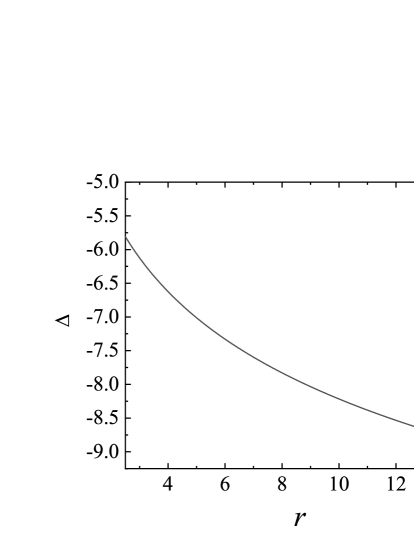
The approximate equivalence between the two black hole black hole gravitational systems in the dynamics of orbits outside the event horizons is due to the two metric functions and having only minor differences. As Eq. (3) shows, the difference between the two metric functions and is as and . In fact, Fig. 12(a) describes that the difference is about when belongs to the range and . Given and in Fig. 12(b), the difference is about . Because of such small differences, the RN black hole is not clearly distinguished from the regular RN black hole via the motions of particles or photons outside the event horizons. Thus, the two black holes are basically equivalent in these photon circular orbits, photon spheres outside the event horizons, and constraints of the black hole charges based on the First Image of Sagittarius A∗. Their equivalences are also suitable for the stable circular orbits, innermost stable circular orbits, and regular and chaotic dynamics of charged particles outside the event horizons. However, the two black hole systems are completely different as particles or photons move in the vicinity of the origin . In this case, the metric function is not expanded like Eq. (3). Although we cannot provide the analytical solutions of particles or photons moving near the origin, we easily estimate
| (39) |
Typically larger differences between the two metric functions for smaller values of are also shown in Figs. 12 (c) and (d). Therefore, the RN black hole can be distinguished clearly from the regular RN black hole via such dramatically different changes of the two metric functions in the motions of particles or photons around the origin.
6 Summary
The aforementioned regular black hole is a solution of the Einstein field equations coupled to a suitable NED. It is unlike the RN black hole with curvature singularities, but resembles the RN black hole with horizons. The two black holes satisfy the weak energy condition everywhere and have similar asymptotic behaviors.
When the two black hole systems have the same parameters, they also have the same photon effective potentials, photon circular orbits and photon spheres outside the event horizons. Due to the same photon spheres in the two black hole systems, the black hole shadows and constraints of the black hole charges based on the First Image of Sagittarius A∗ are almost the same.
The radial motions of charged particles outside the horizons of the two magnetized black holes, including the effective potentials, stable circular orbits and innermost stable circular orbits, have no explicit differences. The constructions of explicit symplectic integrators for the off equatorial plane motions of charged particles in the two magnetized black hole systems are different. The splitting and composition methods are easily available for the RN black hole. However, they are not for the regular black hole unless an appropriate time transformation is given to the regular black hole. In fact, such a time-transformed Hamiltonian exists five explicitly integrable splitting pieces. In spite of these differences, the two black hole systems have the same regular and chaotic dynamical features of charged particles. An increase of the magnetic field parameter or the magnitude of negative Coulomb parameter equal to the product of the black hole charge and the particle charge easily induces chaos due to the gravitational effects increasing. However, an increase of the black hole charge or the positive Coulomb parameter weakens the strength of chaos due to the repulsive force effects increasing. The variation of dynamical properties is not very sensitive dependence on an appropriate increase of the black hole charge.
In sum, the basic equivalence between the two black hole spacetimes exists in the photon circular orbits, photon spheres outside the event horizons and constraints of the black hole charges. This equivalence is also suitable for the stable circular orbits, innermost stable circular orbits, and regular and chaotic dynamics of charged particles outside the event horizons. These equivalences in the dynamics of orbits outside the event horizons of the two charged black holes are due to the extremely small differences of the two metric functions. In view of this, the RN black hole can be simulated by using the regular black hole without curvature singularity in some situations.
Data Availability Statements
All data generated or analysed during this study are included in this published article.
Acknowledgments
The authors are grateful to two referees for useful suggestions. This research was supported by the National Natural Science Foundation of China (Grant No. 11973020) and the National Natural Science Foundation of Guangxi (No. 2019JJD110006).
References
- a (2000) [1] L.M. John, W. Moffat, P. Nicolini, Phys. Lett. B 695, 397 (2011)
- a (2000) [2] J.W. Moffat, Phys. Rev. D 56, 6264 (1997)
- a (2000) [3] X.-M. Deng, European Physical Journal C 80 (6), 489 (2020)
- a (2000) [4] B. Gao, X.-M. Deng, European Physical Journal C 81 (11), 983 (2021)
- a (2000) [5] X. Lu, Y. Xie, European Physical Journal C 81, 627 (2021)
- a (2000) [6] T. Clifton, P. F. Ferreira, A. Padilla, C. Skordis, Physics Reports 513, 1 (2012)
- a (2000) [7] X.-M. Deng, European Physical Journal C 80 (6), 489 (2020)
- a (2000) [8] T.-Y. Zhou, Y. Xie, European Physical Journal C 80, 1070 (2020)
- a (2000) [9] J.M. Bardeen, Proceedings of International Conference GR5. Tiflis, U.S.S.R. (1968)
- a (2000) [10] E. Ayón-Beato, A. García, Phys. Rev. Lett. 80, 5056 (1998)
- a (2000) [11] J.W. Moffat, European Physical Journal C 75, 175 (2015)
- a (2000) [12] K.A. Bronnikov, Phys. Rev. D 63, 044005 (2001)
- a (2000) [13] L. Balart, E.C. Vagenas, Phys. Rev. D 90, 124045 (2014)
- a (2000) [14] E. Ayón-Beato, A. García, Gen. Rel. Grav. 37, 635 (2005)
- a (2000) [15] I. Dymnikova, Class. Quant. Grav. 21, 4417 (2004)
- a (2000) [16] X. Lu, Y. Xie, European Physical Journal C 80, 625 (2020)
- a (2000) [17] E. Ayón-Beato, A. García, Phys. Lett. B 464, 25 (1999)
- a (2000) [18] E. Ayón-Beato, A. García, Gen. Rel. Grav. 31, 629 (1999)
- a (2000) [19] E. Ayón-Beato, A. García, Phys. Lett. B 493, 149 (2000)
- a (2000) [20] S.A. Hayward, Phys. Rev. Lett. 96, 031103 (2006)
- a (2000) [21] L. Balart, E. C. Vagenas, Phys. Lett. B 730, 14 (2014)
- a (2000) [22] P. Nicolini, A. Smailagic, E. Spallucci, Phys. Lett. B 632, 547 (2006).
- a (2000) [23] S. Ansoldi, P. Nicolini, A. Smailagic, E. Spallucci, Phys. Lett. B 645, 261 (2007)
- a (2000) [24] I. Dymnikova, Gen. Rel. Grav. 24, 235 (1992)
- a (2000) [25] I. Dymnikovaa, E. Galaktionov, Class. Quant. Grav. 32, 165015 (2015)
- a (2000) [26] A. Jawad, F. Ali, M. Jamil, U. Debnath, Commun. Theor. Phys. 66, 509 (2016)
- a (2000) [27] S. Hussain, M. Jamil, Phys. Rev. D 92, 043008 (2015) bibitemr28 [28] M. Azreg-Aïnou, S. Haroon, M. Jamil, Int. J. Mod. Phys. D 28, 1950063 (2019)
- a (2000) [29] M. Azreg-Aïnou, Z. Chen, B. Deng, M. Jamil, T. Zhu, Q. Wu, Y.-K. Lim, Phys. Rev. D 102, 044028 (2020)
- a (2000) [30] S. Hussain, I. Hussain, M. Jamil, Eur. Phys. J. C 74, 3210 (2014)
- a (2000) [31] K. Akiyama et al. [Event Horizon Telescope Collaboration], Astrophys. J. Lett. 930, L12 (2022)
- a (2000) [32] Y. Wang, W. Sun, F. Liu, X. Wu, Astrophys. J. 909, 22 (2021)
- a (2000) [33] X. Wu, Y. Wang, W. Sun, F. Liu, Astrophys. J. 914, 63 (2021)
- a (2000) [34] O. Kopáček, V. Karas, Astrophys. J. 787, 117 (2014).
- a (2000) [35] H. Yoshida, Phys. Lett. A 150, 262 (1990)
- a (2000) [36] S. Blanes, P.C. Moan, Journal of Computational and Applied Mathematics 142, 313 (2002)
- a (2000) [37] N. Zhou, H. Zhang, W. Liu, X. Wu, The Astrophysical Journal 927, 160 (2022)
- a (2000) [38] X. Wu, T.-Y. Huang, Phys. Lett. A 313, 77 (2003)
- a (2000) [39] X. Wu, T.-Y. Huang, H. Zhang H, Phys. Rev. D 74, 083001 (2000)
- a (2000) [40] C. Froeschlé, E. Lega, Celestial Mechanics and Dynamical Astronomy 78, 167 (2000)
| 1 | 2 | 3 | 4 | 5 | 6 | 7 | 8 | 9 | 10 | |
| 0.96 | 1.95 | 2.94 | 3.92 | 4.87 | 5.85 | 6.84 | 7.82 | 8.78 | 9.76 | |
| 1 | 2 | 3 | 4 | 5 | 6 | 7 | 8 | 9 | 10 |