EPR-Net: Constructing non-equilibrium potential landscape via a variational force projection formulation

Consider an ergodic stochastic differential equation (SDE)

where $\bm{x}_{0}\in\mathbb{R}^{d}$, $\bm{F}:\mathbb{R}^{d}\rightarrow\mathbb{R}^{d}$ is a smooth driving force, $\dot{\bm{w}}=(\dot{w}_{1},\ldots,\dot{w}_{d})^{\top}$ is the $d$-dimensional temporal Gaussian white noise with $\mathbb{E}\dot{w}_{i}(t)=0$ and $\mathbb{E}[\dot{w}_{i}(t)\dot{w}_{j}(s)]=\delta_{ij}\delta(t-s)$ for $i,j=1,\ldots,d$ and $s,t\geq 0$. The constant $D>0$ specifies the noise strength, which is often proportional to the system’s temperature $T$. We denote by $p_{\mathrm{ss}}(\bm{x})$ its steady-state probability density function (PDF).

Following the (T1) type proposal in [3], we define the potential of (1) as $U=-D\ln p_{\mathrm{ss}}$ and the steady probability flux $\bm{J}_{\mathrm{ss}}=p_{\mathrm{ss}}\bm{F}-D\nabla p_{\mathrm{ss}}$ in the domain $\Omega$, which we assume for simplicity is either $\mathbb{R}^{d}$ or a $d$-dimensional hyperrectangle. The steady-state PDF $p_{\mathrm{ss}}(\bm{x})$ satisfies the Fokker-Planck equation (FPE)

and we assume the asymptotic boundary condition (BC) $p_{\mathrm{ss}}(\bm{x})\rightarrow 0$ as $|\bm{x}|\rightarrow\infty$ when $\Omega=\mathbb{R}^{d}$, or the reflecting boundary condition $\bm{J}_{\mathrm{ss}}\cdot\bm{n}=0$ when $\Omega\subset\mathbb{R}^{d}$ is a $d$-dimensional hyperrectangle, where $\bm{n}$ is the unit outer normal. In both cases, we have $p_{\mathrm{ss}}(\bm{x})\geq 0$ and $\int_{\Omega}p_{\mathrm{ss}}(\bm{x})\,\differential\bm{x}=1$.

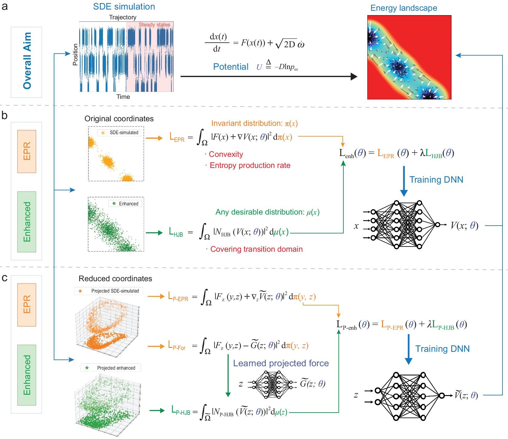
Here we illustrate the main EPR workflow through Fig. 1. As depicted in Fig. 1a, our primary objective is to construct the energy landscape $U=-D\ln p_{\mathrm{ss}}$ defined for Eq. (1). Leveraging our proposed approach, the enhanced EPR method, we first simulate the considered SDEs until steady state is reached in order to get sample points (the whole ‘SDE simulation’ column of Fig. 1). We then train a neural network, representing the potential $U$, for the landscape construction, even when confronted with challenging high-dimensional scenarios. We initially introduce the EPR loss $\operatorname{L_{EPR}}$ (the middle column of Fig. 1b), which benefits from its convexity, with its minimum coinciding with the entropy production rate. Subsequently, we present the enhanced EPR loss $\operatorname{L_{enh}}$, tailored to encompass the transition domain more effectively. Furthermore, the overall methodology can be easily extended to the dimensionality reduction problem (Fig. 1c), with a unified formulation as the EPR framework shown in Fig. 1b, but for the projected variables and corresponding loss functions $\operatorname{L_{P-EPR}}$ and $\operatorname{L_{P-enh}}$.

Aiming at an effective approach for high-dimensional applications, we employ NNs to approximate $U(\bm{x})$, and the key idea in this paper is to learn $U$ by training DNN with the loss function

where $V:=V(\bm{x};\theta)$ is a neural network function with parameters $\theta$ [28], and $\differential\pi(\bm{x})=p_{\mathrm{ss}}(\bm{x})\,\differential\bm{x}$. To justify (3), we note that, for any function $W$, $U$ satisfies the orthogonality relation

which follows from FPE (2), a simple integration by parts and the corresponding BC. Equation (4) means that $\bm{F}+\nabla U$ is perpendicular to the space $\mathcal{G}$ formed by $\nabla W$ for all possible $W$ under the $\pi$-weighted inner product. Equivalently, $-\nabla U$ is the orthogonal projection of the driving force $\bm{F}$ onto $\mathcal{G}$ under the $\pi$-weighted inner product, which implies that $U$ is the unique minimizer (up to a constant) of the loss function (3). See Supplementary Information (SI) Section A for derivations in detail. We note that related ideas are taken in coarse-graining of molecular systems [29, 30] and generative modeling in machine learning [31, 32]. However, to the best of our knowledge, using the loss in (3) to construct the potential of NESS systems has never been considered before.

In fact, define the $\pi$-weighted inner product for any square integrable functions $f,g$ on $\Omega$ as

and the corresponding $L^{2}_{\pi}$-norm $\|\cdot\|_{\pi}$ by $\|f\|^{2}_{\pi}:=(f,f)_{\pi}$, we get a Hilbert space $L^{2}_{\pi}$ (see, e.g., [33, Chapter II.1]). Eq. (4) implies that the minimization of EPR loss finds the orthogonal projection of $\bm{F}$ to the function gradient space $\mathcal{G}$, which is formed by function gradients $\nabla W$ for any $W$, under the $\pi$-weighted inner product. Choosing $W=U$ in (4) gives

However, we remark that this orthogonality holds only in the $L^{2}_{\pi}$-inner product sense instead of the pointwise sense. Furthermore, the two orthogonality relations (4) and (6) can be understood as follows. Using (6), relation (4) is equivalent to $\int_{\Omega}\bm{l}\cdot\nabla Wd\pi=0$ for any $W$. Integration by parts gives $\nabla\cdot(\bm{l}\,\mathrm{e}^{-U/D})=0$, which is equivalent to $\nabla U\cdot\bm{l}+D\nabla\cdot\bm{l}=0$. When $D\rightarrow 0$, we recover the pointwise orthogonality, which is adopted in computing quasi-potentials in [24]. In mathematical language, (6) can be understood as the Hodge-type decomposition in $L^{2}_{\pi}$ instead of $L^{2}$ space.

To utilize (3) in numerical computations, we replace the ensemble average (3) with respect to the unknown $\pi$ by the empirical average with data sampled from (1):

Here $(\bm{x}_{i})_{1\leq i\leq N}$ could be either the final states (at time $\mathsf{T}$) of $N$ independent trajectories starting from different initializations, or equally spaced time series along a single long trajectory up to time $\mathsf{T}$, where $\mathsf{T}\gg 1$. In both cases, the ergodicity of SDE in (1) guarantees that (7) is a good approximation of (3) as long as $\mathsf{T}$ is large [34]. We adopt the former approach in the numerical experiments in this work, where the gradients of both $V$ (with respect to $\bm{x}$) and the loss itself (with respect to $\theta$) in (7) are calculated by auto-differentiation through PyTorch [35]. Given the involvement of an approximation on $\pi$, we perform a formal stability analysis of (3) in SI Section B to ensure its reliability and robustness. Additionally, in the following subsection, we elucidate the benefits of EPR, particularly in terms of convexity and its physical interpretation pertaining to the entropy production rate.

The minimum loss of (3), denoted as $\operatorname{L_{EPR}}(U)$, possesses a well-defined physical interpretation. In the following discussion, we show that this minimum EPR loss aligns precisely with the steady entropy production rate as defined in the NESS theory. Following [36, 37], we have the important identity concerning the entropy production for (1):

Here $S(t):=-\int_{\Omega}p(\bm{x},t)\ln p(\bm{x},t)\,\differential\bm{x}$ is the entropy of the probability density function $p(\bm{x},t)$ at time $t$, $e_{p}$ is the entropy production rate (EPR)

and $h_{d}$ is the heat dissipation rate

with the probability flux $\bm{J}(\bm{x},t):=p(\bm{x},t)(\bm{F}(\bm{x})-D\nabla\ln p(\bm{x},t))$ at time $t$. When $D=k_{B}T$, the above formulas have clear physical meaning in statistical physics.

From the loss in (3) and the steady state of (9), we get the identity

where $\bm{J}_{\mathrm{ss}}(\bm{x})$ is the steady probability flux and $e^{\rm{ss}}_{p}$ denotes the steady entropy production rate (EPR) of the NESS system (1) [36, 3, 37]. Therefore, minimizing (3) is equivalent to approximating the steady Entropy Production Rate. This correspondence provides a rationale for naming our approach ‘EPR-Net’.

EPR loss has an appealing property that it is strictly convex on $V$ (up to a constant), i.e.,

for any $0<\omega<1$ and $V_{0},V_{1}$ which satisfy $\nabla(V_{0}-V_{1})\not\equiv 0$, where $V_{\omega}:=(1-\omega)V_{0}+\omega V_{1}$. Eq. (12) can be easily verified by direct calculations. This strict convexity guarantees the uniqueness of the critical point $V$ (up to a constant) and provides theoretical guarantee on the fast convergence of the training procedure under certain assumptions [38]. It may also contribute to better convergence behavior of EPR during the training process, as mentioned in the numerical comparisons part.

Substituting the relation $p_{\mathrm{ss}}(\bm{x})=\exp(-U(\bm{x})/D)$ into (2), we get the viscous HJB equation

with the asymptotic BC $U\rightarrow\infty$ as $|\bm{x}|\rightarrow\infty$ in the case of $\Omega=\mathbb{R}^{d}$, or the reflecting BC $(\bm{F}+\nabla U)\cdot\bm{n}=0$ on $\partial\Omega$ when $\Omega$ is a $d$-dimensional hyperrectangle, respectively. As in the framework of PINNs [26], (13) motivates the HJB loss

where $\mu$ is any desirable distribution. By choosing $\mu$ properly, this loss allows the use of sample data that better covers the domain $\Omega$ and, when combined with the loss in (3), leads to improvement of the training results when $D$ is small. Specifically, for small $D$, we propose the enhanced loss which has the form

where $\operatorname{\widehat{L}_{EPR}}(\theta)$ is defined in (7), $\operatorname{\widehat{L}_{HJB}}(\theta)=\frac{1}{N^{\prime}}\sum_{i=1}^{N^{\prime}}|\mathcal{N}_{\textrm{HJB}}(V(\bm{x}^{\prime}_{i};\theta))|^{2}$ is an approximation of (14) using an independent data set $(\bm{x}^{\prime}_{i})_{1\leq i\leq N^{\prime}}$ obtained by sampling the trajectories of (1) with a larger $D^{\prime}>D$. The weight parameter $\lambda>0$ balances the contribution of the two terms in (15). While its value can be tuned based on system’s properties, in our numerical experiment we observed that the method performs well for $\lambda$ taking values in a relatively broad range. Note that the proposed strategy is both general and easily adaptable. For instance, one can alternatively use data $(\bm{x}^{\prime}_{i})_{1\leq i\leq N^{\prime}}$ that contains more samples in the transition region, or employ in (15) a modification of the loss (14) [22]. We further illustrate the motivation of enhanced EPR in SI Section E.

Within this subsection, we undertake a comparative analysis of 2D benchmark problems. These encompass a toy model, a 2D biological system exhibiting a limit cycle [3], and a 2D multi-stable system [5], see SI Section F.1-F.4 for training details, additional results and problem settings.

We apply our landscape construction approach to the 3D Lorenz system [42] with isotropic temporal Gaussian white noise, i.e. the system (1) with $\bm{F}=(F_{x},F_{y},F_{z})$ and

where $\beta_{1}=10,\beta_{2}=28$, and $\beta_{3}=\frac{8}{3}$. We add the noise with strength $D=1$. This model was also considered in [23] with $D=20$. We obtain the enhanced data $(\bm{x}^{\prime}_{i})_{1\leq i\leq N^{\prime}}$ by adding Gaussian noises with standard deviation $\sigma=5$ to the SDE-simulated data $(\bm{x}_{i})_{1\leq i\leq N}$, where $N=N^{\prime}=10000$. We directly train the 3D potential $V(\bm{x};\theta)$ by enhanced EPR (16) with $\lambda_{1}=10.0,\lambda_{2}=1.0$, using Adam with a learning rate of 0.001 and batch size of 2048. A slice view of the landscape is presented in Fig. 4a and the learned 3D potential agrees well with the simulated samples.

To further validate the efficacy of EPR-Net in high-dimensional scenarios, we construct a Gaussian mixture model (GMM) in $\mathbb{R}^{12}$ with two centers, of which the true solution can be denoted as $U_{0}(\bm{x})=-D\log p_{0}(\bm{x})$, where $p_{0}(\bm{x})=w_{1}p_{1}(\bm{x})+w_{2}p_{2}(\bm{x})$, and $p_{i}(\bm{x})=Z_{i}^{-1}\exp(-(\bm{x}-\bm{\mu}_{i})^{T}\Sigma_{i}^{-1}(\bm{x}-\bm{\mu}_{i})/2),i=1,2$, with normalization factor $Z_{i}$. The parameters are chosen as $w_{1}=0.6$, $w_{2}=0.4$, $\bm{\mu}_{1}=(1.2,2.0,0.6,1.5,0.9,1.5,1.5,0.9,1.2,1.2,0.5$, $1.8)^{\top}$, $\bm{\mu}_{2}=(1.8,1.4,0.8,0.9,0.9,1.5,2.0,1.0$, $1.6,1.0,0.7,1.4)^{\top}$, $\Sigma_{1}=0.04I$, and $\Sigma_{2}=0.02I$.

For evaluation, we first sample 10,000 points from the known GMM distribution and calculate the relative error between the learned 12D potential $V(\bm{x};\theta^{*})$ and the true potential $U_{0}(\bm{x})$. The resulting rRMSE and rMAE are 0.054 and 0.051, respectively, indicating the high accuracy of the learned potential. In addition, we denote the first two dimensions of this 12D problem as $(x_{1},x_{2})$ and draw samples from the corresponding conditional distribution $p_{0}(\bm{x}|x_{1},x_{2})$. As depicted in Fig. 4b, we compute the cumulative measure of the absolute error between $U_{0}(\bm{x})$ and the learned solution $V(\bm{x})$ based on the conditional distribution as $\int|U_{0}(\bm{x})-V(\bm{x})|p_{0}(\bm{x}|x_{1},x_{2})\differential\bm{x}$. Impressively, this integral consistently remains below 0.01, underscoring the fact that our approach yields negligible errors in the effective domain. Moreover, comparing the barrier heights (BHs) further validates the precision of our approach, with a relative error of less than 5% for both BHs. Due to the diagonal covariance matrix, the saddle point precisely lies on the line passing through $\bm{\mu}_{1}$ and $\bm{\mu}_{2}$, allowing us to directly compare the BHs. As shown in Fig 4c, the true and computed slice lines coincide well. For additional details, please refer to SI Section F.5.

Subsequently, we apply our dimensionality reduction approach to construct the landscape for an 8D cell cycle model [4], which contains both a limit cycle and a stable equilibrium point. In this case, we consider CycB (a cyclin B protein) and Cdc20 (an exit protein) as the reduced variables following [4]. As shown in Fig. 5a and b, we can find that both the profile of the reduced potential and the force strength agree well with the density of projected samples. Moreover, we gain some important insights from Fig. 5b on the projection of the high-dimensional dynamics to two dimensions. One particular feature is that the limit cycle induced by the projected force $\widetilde{\bm{G}}(\bm{x};\theta^{*})$ (outer red circle) slightly differs from the limit cycle directly projected from high dimensions (yellow circle), and the difference is either minor or moderate depending on whether the sample density near the limit circle is high or low. This is natural in the reduction when $D>0$, since the distribution $\pi(\bm{y}|\bm{z})$ involved in computing $\widetilde{\bm{G}}(\bm{x};\theta^{*})$ is not a Dirac $\delta$-distribution, but a diffusive distribution with varying widths along the limit cycle, and the difference will disappear as $D\rightarrow 0$. Another feature is that we unexpectedly get an additional stable limit cycle (inner red circle) and a stable point (red dot in the center) emerging inside the outer limit cycle. Though virtual in high dimensions and biologically irrelevant, the existence of such two limit sets is reminiscent of the Poincaré-Bendixson theorem in planar dynamics theory [46, Chapter 10.6], which depicts a common phenomenon when performing dimensionality reduction with limit cycles to the 2D plane. Note that this theorem does not guarantee the stability of such fixed points; they could be stable, unstable, or even saddle points, see another case in SI G.1. The emergence of these two limit sets is specific in this model due to the relatively flat landscape of the potential in the centering region. In addition, close to the saddle point of $\widetilde{V}$ (green star), there is a barrier along the limit cycle direction, while there is a local well along the Cdc20 direction, which characterizes the region that biological cycle paths mainly go through. Last but not least, an enlarged view of the local attractive domain outside the limit cycle shows its intricate spiral structure (Fig. 5c), which has not been revealed in previous work based on mean-field approximation [4].

We compare two approaches to construct the reduced potential. One is to learn the reduced force $\widetilde{\bm{G}}(\bm{z};\theta^{*})$ by (26) first and then use it to construct the landscape $\widetilde{V}(\bm{z};\theta^{*})$ by enhanced EPR in $\bm{z}$-space. The other is to build a high-dimensional potential $V(\bm{x};\theta^{*})$ by enhanced EPR first and then reduce it (see SI Section C.1). For this comparison, we apply our approach to a gene stem cell regulatory network described by an ODE in 52 dimensions [27] and take GATA6 (a major differentiation marker gene) and NANOG (a major stem cell marker gene) as the reduced variable $\bm{z}$, as suggested in [27]. We define $\mathcal{A}_{i}$ as the set of indices for activating $x_{i}$ and $\mathcal{R}_{i}$ as the set of indices for repressing $x_{i}$, the corresponding relationships are defined as the 52D node network shown in [27]. For $i=1,...,52$,

where $a=0.37$, $b=0.5$, $k=1$, $S=0.5$, and $n=3$. We choose the noise strength $D=0.02$ and focus on the domain $\Omega=[0,3]^{52}$.

As shown in Fig. 5d, the projected force $\widetilde{\bm{G}}(\bm{z};\theta^{*})$ demonstrates the reduced dynamics and the constructed potential $\widetilde{V_{1}}(\bm{z};\theta^{*})$ agrees well with the SDE-simulated samples. While $\widetilde{V_{1}}(\bm{z};\theta^{*})$ is learned by first obtaining the projected force, $\widetilde{V_{2}}(\bm{z};\theta^{*})$ is reduced from a high-dimensional ${V}(\bm{x};\theta^{*})$ precomputed by enhanced EPR. The gray plot of the absolute error of $|\widetilde{V_{1}}(\bm{z};\theta^{*})-\widetilde{V_{2}}(\bm{z};\theta^{*})|$ is shown in Fig. 5e, which supports the consistency of two potentials learned by different approaches. When taking $\widetilde{V_{1}}(\bm{z};\theta^{*})$ as the reference solution, we get the rRMSE 0.113 and rMAE 0.097. The minor relative errors show that these two approaches to constructing the reduced potential are quantitatively consistent, although it is difficult to know which is more accurate. It also indirectly supports the reliability of the learned high-dimensional potential $V(\bm{x};\theta^{*})$. The obtained landscape shows a smoother and more delicate profile compared to the mean-field approach [27].

References

- [1] Waddington C. The strategy of the genes 1957.
- [2] Ao P. Potential in stochastic differential equations: novel construction. J. Phys. A-Math. Gen. 2004; 37: L25.
- [3] Wang J, Xu L and Wang E. Potential landscape and flux framework of nonequilibrium networks: Robustness, dissipation, and coherence of biochemical oscillations. Proc. Nat. Acad. Sci. USA 2008; 105: 12271.
- [4] Wang J, Li C and Wang E. Potential and flux landscapes quantify the stability and robustness of budding yeast cell cycle network. Proc. Nat. Acad. Sci. USA 2010; 107: 8195.
- [5] Wang J, Zhang K, Xu L et al. Quantifying the Waddington landscape and biological paths for development and differentiation. Proc. Nat. Acad. Sci. USA 2011; 108: 8257.
- [6] Zhou J, Aliyu M, Aurell E et al. Quasi-potential landscape in complex multi-stable systems. J. R. Soc., Interface 2012; 9: 3539.
- [7] Ge H and Qian H. Landscapes of non-gradient dynamics without detailed balance: Stable limit cycles and multiple attractors. Chaos 2012; 22: 023140.
- [8] Lv C, Li X, Li F et al. Constructing the energy landscape for genetic switching system driven by intrinsic noise. PLoS ONE 2014; 9: e88167.
- [9] Shi J, Aihara K, Li T et al. Energy landscape decomposition for cell differentiation with proliferation effect. Nat. Sci. Rev. 2022; 9: nwac116.
- [10] Maier RS and Stein DL. Escape problem for irreversible systems. Phys. Rev. E 1993; 48: 931.
- [11] Aurell E and Sneppen K. Epigenetics as a first exit problem. Phys. Rev. Lett. 2002; 88: 048101.
- [12] Sasai M and Wolynes P. Stochastic gene expression as a many-body problem. Proc. Nat. Acad. Sci. USA 2003; 100: 2374.
- [13] Roma DM, O’Flanagan RA, Ruckenstein AE et al. Optimal path to epigenetic switching. Phys. Rev. E 2005; 71: 011902.
- [14] Ferrell JEJ. Bistability, bifurcations, and Waddington’s epigenetic landscape. Curr. Biol. 2012; 22: R458.
- [15] Wang J. Landscape and flux theory of non-equilibrium dynamical systems with application to biology. Adv. Phys. 2015; 64: 1.
- [16] Zhou P and Li T. Construction of the landscape for multi-stable systems: Potential landscape, quasi-potential, A-type integral and beyond. J. Chem. Phys. 2016; 144: 094109.
- [17] Yuan R, Zhu X, Wang G et al. Cancer as robust intrinsic state shaped by evolution: a key issues review. Rep. Prog. Phys. 2017; 80: 042701.
- [18] Fang X, Kruse K, Lu T et al. Nonequilibrium physics in biology. Rev. Mod. Phys. 2019; 91: 045004.
- [19] Li C, Hong T and Nie Q. Quantifying the landscape and kinetic paths for epithelial–mesenchymal transition from a core circuit. Phys. Chem. Chem. Phys. 2016; 18: 17949–56.
- [20] Cameron M. Finding the quasipotential for nongradient SDEs. Phys. D 2012; 241: 1532.
- [21] Li C and Wang J. Landscape and flux reveal a new global view and physical quantification of mammalian cell cycle. Proc. Nat. Acad. Sci. USA 2014; 111: 14130.
- [22] Lin B, Li Q and Ren W. Computing the invariant distribution of randomly perturbed dynamical systems using deep learning. J. Sci. Comp. 2022; 91: 77.
- [23] Lin B, Li Q and Ren W. Computing high-dimensional invariant distributions from noisy data. J. Comp. Phys. 2023; 474: 111783.
- [24] Lin B, Li Q and Ren W. A data driven method for computing quasipotentials. Proc. Mach. Learn. Res., volume 145 of 2nd Annual Conference on Mathematical and Scientific Machine Learning (2021) 652.
- [25] Crandall MG and Lions PL. Viscosity solution of Hamilton-Jacobi equations. Trans. Amer. Math. Soc. 1983; 277: 1.
- [26] Raissi M, Perdikaris P and Karniadakis GE. Physics-informed neural networks: A deep learning framework for solving forward and inverse problems involving nonlinear partial differential equations. J. Comp. Phys. 2019; 378: 686.
- [27] Li C and Wang J. Quantifying cell fate decisions for differentiation and reprogramming of a human stem cell network: Landscape and biological paths. PLoS Comput. Biol. 2013; 9: e1003165.
- [28] Goodfellow I, Bengio Y and Courville A. Deep learning 2016.
- [29] Zhang L, Han J, Wang H et al. DeePCG: Constructing coarse-grained models via deep neural networks. J. Chem. Phys. 2018; 149: 034101.
- [30] Husic BE, Charron NE, Lemm D et al. Coarse graining molecular dynamics with graph neural networks. J. Chem. Phys. 2020; 153: 194101.
- [31] Hyvärinen A. Estimation of non-normalized statistical models by score matching. J. Mach. Learn. Res. 2005; 6: 695–709.
- [32] Song Y and Ermon S. Generative modeling by estimating gradients of the data distribution. Wallach H, Larochelle H, Beygelzimer A et al., editors, Advances in Neural Information Processing Systems, volume 32 of NeurIPS (2019) 11918–30.
- [33] Courant R and Hilbert D. Methods of mathematical physics 1953.
- [34] Khasminskii R. Stochastic stability of differential equations 2012.
- [35] Paszke A, Gross S, Massa F et al. Pytorch: An imperative style, high-performance deep learning library. Advances in Neural Information Processing Systems, volume 32 of NeurIPS (2019) 8024.
- [36] Qian H. Mesoscopic nonequilibrium thermodynamics of single macromolecules and dynamic entropy-energy compensation. Phys. Rev. E 2001; 65: 016102.
- [37] Zhang X, Qian H and Qian M. Stochastic theory of nonequilibrium steady states and its applications. part i. Phys. Rep. 2012; 510: 1–86.
- [38] Mei S, Montanari A and Nguyen PM. A mean field view of the landscape of two-layer neural networks. Proc. Nat. Acad. Sci. USA 2018; 115: E7665–E71.
- [39] Kobyzev I, Prince SJD and Brubaker M. Normalizing flows: An introduction and review of current methods. IEEE Trans. Patt. Anal. Mach. Intel. 2021; 43: 3964–79.
- [40] Zhu XM, Yin L and Ao P. Limit cycle and conserved dynamics. International Journal of Modern Physics B 2006; 20: 817–27.
- [41] Ma Y, Tan Q, Yuan R et al. Potential function in a continuous dissipative chaotic system: Decomposition scheme and role of strange attractor. International Journal of Bifurcation and Chaos 2014; 24: 1450015.
- [42] Lorenz EN. Deterministic nonperiodic flow. J. Atmos. Sci. 1963; 20: 130–41.
- [43] Zhang W, Hartmann C and Schütte C. Effective dynamics along given reaction coordinates, and reaction rate theory. Faraday Discuss. 2016; 195: 365–94.
- [44] Kang X and Li C. A dimension reduction approach for energy landscape: Identifying intermediate states in metabolism-emt network. Adv. Sci. 2021; 8: 2003133.
- [45] Ferrell JE, Tsai TYC and Yang Q. Modeling the cell cycle: Why do certain circuits oscillate? Cell 2011; 144: 874–85.
- [46] Hirsch MW, Smale S and Devaney RL. Differential equations, dynamical systems, and an introduction to chaos 2004.
- [47] Bonati L, Zhang YY and Parrinello M. Neural networks-based variationally enhanced sampling. Proc. Nat. Acad. Sci., USA 2019; 116: 17641–7.
- [48] Bonati L, Rizzi V and Parrinello M. Data-driven collective variables for enhanced sampling. J. Phys. Chem. Lett. 2020; 11: 2998–3004.
- [49] Evans LC. Partial differential equations 2010.
- [50] Holmes MH. Introduction to perturbation methods 2013.
- [51] Frenkel D and Smit B. Understanding molecular simulation: From algorithms to applications 2002.
- [52] Kingma DP and Ba J. Adam: a method for stochastic optimization. Proceedings of the International Conference on Learning Representations (2015) .
- [53] Durkan C, Bekasov A, Murray I et al. Neural spline flows. Advances in Neural Information Processing Systems, volume 32 of NeurIPS (2019) .
Supplementary Information for EPR-Net:
Constructing non-equilibrium potential landscape via a variational force projection formulation
In this supplementary information (SI), we will present further theoretical derivations and computational details of the contents in the main text (MT). This SI consists of two parts: theory and computation.
PART 1: THEORY
We will first provide details of theoretical derivations omitted in the MT.
Appendix A Derivation of the EPR loss
In this section, we show that, up to an additive constant, the potential function is the unique minimizer of the EPR loss in equation (1) in MT.
First, we show that the orthogonality relation