Environmental dependence of Type IIn supernova properties
Type IIn supernovae occur when stellar explosions are surrounded by dense hydrogen-rich circumstellar matter. The dense circumstellar matter is likely formed by extreme mass loss from their progenitors shortly before they explode. The nature of Type IIn supernova progenitors and the mass-loss mechanism forming the dense circumstellar matter are still unknown. In this work, we investigate if there are any correlations between Type IIn supernova properties and their local environments. We use Type IIn supernovae with well-observed light-curves and host-galaxy integral field spectroscopic data so that we can estimate both supernova and environmental properties. We find that Type IIn supernovae with a higher peak luminosity tend to occur in environments with lower metallicity and/or younger stellar populations. The circumstellar matter density around Type IIn supernovae is not significantly correlated with metallicity, so the mass-loss mechanism forming the dense circumstellar matter around Type IIn supernovae might be insensitive to metallicity.
Key Words.:
supernovae: general – stars: massive – stars: mass-loss| Name | Redshift | Distance Modulus | Rise time | Peak mag.aaaaHost galaxy extinction is not taken into account. | Mass-loss ratebbbbA wind velocity of 100 is assumed. | Referencecccc(1) Van Dyk et al. (2000), (2) Poon et al. (2011), (3) Kiewe et al. (2012), (4) Hicken et al. (2017), (5) Nyholm et al. (2020), (6) Dong et al. (2015); Shappee et al. (2015), (7) Pastorello et al. (2018), (8) Tonry et al. (2016); Takats et al. (2016), (9) Brimacombe et al. (2016c); Elias-Rosa et al. (2016), (10) Brimacombe et al. (2016a); Reynolds et al. (2016), (11) Brimacombe et al. (2016b); Brown et al. (2016), (12) Tonry et al. (2017a); Barbarino et al. (2017), (13) Tonry et al. (2017b); Onori et al. (2017), (14) Tonry et al. (2017c); Pan (2017), (15) Xu et al. (2017); Lyman et al. (2017), (16) Moller et al. (2017); Lyman et al. (2017), (17) Kumar et al. (2019); Smith & Andrews (2020); Chandra et al. (2022); Moran et al. (2023), (18) Tonry et al. (2021); Pessi et al. (2021) | |
|---|---|---|---|---|---|---|---|
| mag | days | mag | |||||
| SN 1997bs | ddddWillick & Batra (2001) | (1) | |||||
| SN 1998S | eeeeSorce et al. (2014) | (2) | |||||
| SN 2005cl | ffffSpringob et al. (2014) | (3) | |||||
| SN 2005db | eeeeSorce et al. (2014) | (3) | |||||
| SN 2005kd | eeeeSorce et al. (2014) | (4) | |||||
| SN 2007cm | ggggTheureau et al. (2007) | (4) | |||||
| SN 2008B | hhhhTully et al. (2013) | (4) | |||||
| SN 2015Z | ggggTheureau et al. (2007) | (5) | |||||
| ASASSN-15ab | iiiiDM from redshift. | (6) | |||||
| SN 2016bdu | iiiiDM from redshift. | (7) | |||||
| SN 2016iaf | iiiiDM from redshift. | (8) | |||||
| ASASSN-16bw | iiiiDM from redshift. | (9) | |||||
| ASASSN-16in | iiiiDM from redshift. | (10) | |||||
| ASASSN-16jt | iiiiDM from redshift. | (11) | |||||
| SN 2017bzm | iiiiDM from redshift. | (12) | |||||
| SN 2017cin | iiiiDM from redshift. | (13) | |||||
| SN 2017fav | iiiiDM from redshift. | (14) | |||||
| SN 2017ggv | iiiiDM from redshift. | (15) | |||||
| SN 2017ghw | iiiiDM from redshift. | (16) | |||||
| SN 2017hcc | iiiiDM from redshift. | (17) | |||||
| SN 2021fpn | iiiiDM from redshift. | (18) |
1 Introduction
Type IIn supernovae (SNe IIn) occur when stars explode within a dense hydrogen-rich circumstellar matter (CSM, Schlegel 1990; Filippenko 1997). The dense CSM is created by strong mass loss from the progenitors with typical mass-loss rate estimates of more than (e.g., Taddia et al., 2013; Kiewe et al., 2012; Moriya et al., 2014; Ofek et al., 2014a). Such mass-loss rates are much higher than those measured for typical stars (e.g., Smith, 2014), and the progenitors and mass-loss mechanisms of SNe IIn are still not well understood. It is suggested that the high mass-loss rates are similar to those of massive () luminous blue variable stars (LBVs, e.g., Weis & Bomans 2020). Indeed, the progenitor of the Type IIn SN 2005gl is consistent with a massive LBV (Gal-Yam & Leonard, 2009). On the other hand, the progenitor of the Type IIn SN 2008S was relatively low mass (, Prieto et al. 2008). These events suggest that progenitors and mass-loss mechanisms of SNe IIn are diverse. In addition, SNe Ia are sometimes hidden below dense hydrogen-rich CSM and observed as SNe IIn (“SN Ia-CSM,” e.g., Sharma et al., 2023).
The local environments where SNe explode provide rich information on their progenitors (see Anderson et al. 2015 for a review). For example, SNe II and Ibc but not SNe Ia preferentially occur in star-forming environments, which indicates that SNe II and Ibc are associated with massive star explosions (e.g., Li et al., 2011; Galbany et al., 2014). There have been several studies of the local environments of SNe IIn. Habergham et al. (2014) found that their locations are not necessarily associated with the most actively star-forming regions in their host galaxies and some may not be associated with very massive progenitors. A later study by Ransome et al. (2022) found that 60% of SNe IIn originate from actively star-forming regions and could be linked to very massive progenitors such as LBVs. The remaining 40% were not correlated with ongoing star formation and could have relatively low-mass progenitors (see also Kuncarayakti et al., 2018). Similarly, Galbany et al. (2018) estimated the age distributions of SN IIn progenitors based on spectra of their surroundings and found that they may have a bimodal age distribution with one peak at and the other at . These studies suggest that SN IIn progenitors are a mixture of massive ( like LBVs) and low-mass ( like the progenitor of SN 2008S) stars. Other local properties may also provide information on their nature. For example, Taddia et al. (2015) investigated the relationship between SN IIn progenitor mass-loss rates and their local metallicity. They found that the progenitors of SNe IIn may have higher mass-loss rates in higher metallicity environments.
In this work, we explore the environmental dependence of SN IIn properties by using SNe IIn with integral-field spectroscopy (IFS) of their host galaxies. The IFS data allow us to estimate not only the metallicity but also environmental parameters such as the local star-formation rates (SFRs). We introduce our SN IIn samples in Section 2. We estimate the local environmental parameters of the SN IIn explosion sites in Section 3 and estimate the SN IIn properties in Section 4. We investigate possible correlations between the environmental and SN properties in Section 5 and discuss them in Section 6. We conclude this paper in Section 7. We adopt a CDM cosmology with , , and (Hinshaw et al., 2013).
| Name | |||
|---|---|---|---|
| SN 1997bs | |||
| SN 1998S | |||
| SN 2005cl | |||
| SN 2005db | |||
| SN 2005kd | |||
| SN 2007cm | |||
| SN 2008B | |||
| SN 2015Z | |||
| ASASSN-15ab | |||
| SN 2016bdu | |||
| SN 2016iaf | |||
| ASASSN-16bw | |||
| ASASSN-16in | |||
| ASASSN-16jt | |||
| SN 2017bzm | |||
| SN 2017cin | |||
| SN 2017fav | |||
| SN 2017ggv | |||
| SN 2017ghw | |||
| SN 2017hcc | |||
| SN 2021fpn |
| Name | EW(H) | |||||
|---|---|---|---|---|---|---|
| Å | years | mag | mag | |||
| SN 1997bs | ||||||
| SN 1998S | ||||||
| SN 2005cl | ||||||
| SN 2005db | ||||||
| SN 2005kd | ||||||
| SN 2007cm | ||||||
| SN 2008B | ||||||
| SN 2015Z | ||||||
| ASASSN-15ab | ||||||
| SN 2016bdu | ||||||
| SN 2016iaf | ||||||
| ASASSN-16bw | ||||||
| ASASSN-16in | ||||||
| ASASSN-16jt | ||||||
| SN 2017bzm | ||||||
| SN 2017cin | ||||||
| SN 2017fav | ||||||
| SN 2017ggv | ||||||
| SN 2017ghw | ||||||
| SN 2017hcc | ||||||
| SN 2021fpn |
2 Sample definition
We constructed our sample using all galaxies observed with IFS from the PISCO, AMUSING, and MaNGA surveys to host a Type IIn SN.
The PMAS/PPak Integral field Supernova hosts COmpilation (PISCO; Galbany et al. 2018) is a compilation of IFS observations of more than 400 SN host galaxies obtained with the Potsdam Multi Aperture Spectograph (PMAS; Roth et al. 2005) on the 3.5m telescope of the Centro Astronomico Hispano-Aleman (CAHA) at the Calar Alto Observatory. The observations were obtained in PPak mode (Verheijen et al., 2004; Kelz et al., 2006). About a third of the objects were observed by the CALIFA survey (Sánchez et al., 2016). Each observation consists of a 3D datacube with a 100% covering factor within a hexagonal field-of-view (FoV) of 1.3 arcmin2, with 1”1” spatial pixels (spaxel) and a spectral resolution of 6 Å over the wavelength range 37507300 Å, providing 4000 spectra per object.
The All-weather MUse Supernova Integral-field of Nearby Galaxies (AMUSING; Galbany et al. 2016a; López-Cobá et al. 2020; Galbany et al. in prep.) survey has been running for 11 semesters (P95-P106), and has compiled observations for more than 800 nearby SN host galaxies with the Multi-Unit Spectroscopic Explorer (MUSE; Bacon et al. 2014), located at the Nasmyth B focus of Yepun, the VLT UT4 telescope at Cerro Paranal Observatory. MUSE is composed of 24 identical IFS. Wide Field Mode (WFM) samples a nearly contiguous 1 arcmin2 FoV with spaxels of 0.2 0.2 arcsec, and over a wavelength range of 4650-9300 Å with a mean resolution of R3000. Each 3D cube consists of 100,000 spectra per pointing.
The Mapping Nearby Galaxies at APO (MaNGA; Bundy et al. 2015) was part of Sloan Digital Sky Survey (SDSS) IV (Blanton et al. 2017) and obtained IFS data of 10,000 nearby galaxies using 17 units of different hexagonal FoVs ranging from 12 to 32 arcsec in diameter at the 2.5m SDSS telescope at the Apache Point Observatory, in New Mexico. The square spaxels are of 0.5 arcsec across, with a spectral resoulution of R2000 over a wavelength range of 3600-10000 Å.
After a thorough search of these three datasets, we compiled an initial sample of 66 SN IIn host galaxies where the SN location was within the FoV. Next, we performed a thorough search for public light-curves of the 66 SNe IIn in the literature. For those objects that exploded in 2016 or after, we also used the ATLAS forced photometry service222https://fallingstar-data.com/forcedphot/queue/ to obtain light curves. For those objects that exploded in 2018 or later, we utilized the ZTF forced photometry service333https://ztfweb.ipac.caltech.edu/cgi-bin/requestForcedPhotometry.cgi. From the 24 SNe IIn with publicly available data, only 17 had light-curves with enough quality and sampling during the rise to reliably determine the peak magnitude and rise time from explosion (see Section 4). In addition, we obtained light curves with good sampling from All-Sky Automated Survey for SuperNovae (ASAS-SN, Shappee et al. 2014; Kochanek et al. 2017) and follow-up observations with the Las Cumbres Observatory Global Telescope network (LCOGT) for four additional SNe IIn (ASASSN-15ab, ASASSN-16bw, ASASSN-16in, and ASASSN-16jt). The LCOGT photometry was performed according to the procedures described in Chen et al. (2022). The final 21 SNe IIn in our sample are listed in Table 1.
3 Local environments
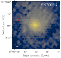
The final sample of 21 SNe IIn is composed of 13 host galaxies observed with MUSE, five with PMAS and three with MaNGA. Synthetic -band images created from the IFS cubes are displayed in Figure 6.
We followed a similar procedure for all 3 IFS instruments. We extracted a rest-frame 2.7 arcsec diameter aperture spectrum for each SN position, corresponding to the worst spatial resolution in all the cubes. We analyzed the spectra as in Galbany et al. (2014, 2016b). We fit single stellar population (SSP) synthesis models to remove the underlying stellar continuum from the ionized gas-phase emission using STARLIGHT (Cid Fernandes et al., 2005, 2009). STARLIGHT determines the fractional contribution of different SSP models to the spectrum, accounting for dust extinction as a foreground screen. We use three parameters from the SSP fit: the stellar mass (), the average light-weighted stellar population age (), and the extinction derived from the stellar component ().
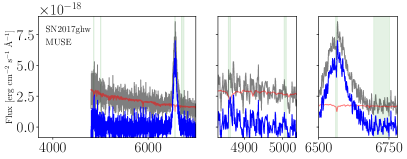
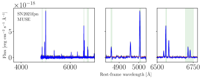
The best fit continuum model is then subtracted from each observed spectrum to leave the ionized gas-phase emission. Figure 7 shows the aperture spectra, the best SSP fits, and their resulting gas-phase emission line spectra for all 21 SN IIn environments. We fit the emission lines needed to estimate oxygen abundances using several different methods. This included fitting Gaussian profiles to the Balmer H 6563 and H 4861 lines, and the [O iii] 5007, [N ii] 6583, [S ii] 6716,31 lines. The H and [N ii] lines were fit simultaneously with [N ii] 6548 as three Gaussian profiles with fixed positions and similar width, but free amplitudes. In seven cases of relatively recent SNe (SN 2016bdu, SN 2016iaf, ASASSN-16bw, ASASSN-16in, ASASSN-16jt, SN 2017ghw, SN 2017hcc; see Figure 7) it was necessary to include a fourth component to account for a broad underlying H emission coming from the CSM interaction (see also Martínez-Rodríguez in prep.).
The flux of the emission lines was corrected for dust extinction along the line of sight using the color excess () estimate from the H/H Balmer line flux ratios assuming the Case B recombination intrinsic ratio for K and an electron density of cm-3 (Osterbrock & Ferland, 2006), and a Fitzpatrick (1999) extinction law.
The ongoing SFR can be directly estimated from the extinction-corrected H flux following Kennicutt (1998),
| (1) |
where
| (2) |
is the extinction-corrected H luminosity in units of erg s-1 and is the luminosity distance to the galaxy. The SFR density () is obtained by dividing the SFR by the area of the aperture in kpc2, and the specific SFR (sSFR) is obtained by dividing the SFR by the stellar mass obtained from the STARLIGHT fit.
While the H flux is an indicator of the ongoing SFR, the H equivalent width, EW(H), is a measurement of how strong the emission line is compared with the stellar continuum. The stellar continuum is dominated by the contribution from old stars, which also contain most of the stellar mass. The EW(H) represents the fraction of young stars, and it can be thought of as an indicator of the strength of the ongoing SFR compared with the past SFR and it decreases with time if no ongoing star-formation is present. It is a reliable proxy for the age of the youngest stellar components (Kuncarayakti et al., 2016; Sánchez et al., 2015). To estimate EW(H), we divided the observed spectrum by the STARLIGHT fit, and repeated the weighted nonlinear least-squares fit of the H line in the normalized spectra.
The most commonly used metallicity indicator in interstellar medium (ISM) studies is the oxygen abundance, since it is the most abundant metal in the gas phase and has very strong optical nebular lines. We estimated the oxygen abundances, , using three different empirical calibrations based on emission-line ratios. In particular, we used the N2 index with the Marino et al. (2013) calibrations updated from Pettini & Pagel (2004) based on the [N ii]/H ratio,
| (3) |
and the O3N2 index based on the difference between the logs of the [O iii]/H and [N ii]/H ratios,
| (4) |
Finally, we used the sulphur-based calibrator from Dopita et al. (2016) based on the [S ii]/H and [N ii]/H ratios,
| (5) |
where . All these calibrations are quite insensitive to extinction because the emission lines used for the ratio diagnostics are close in wavelength. The ratios are also little affected by differential atmospheric refraction (DAR), although DAR has been corrected for during data reduction. The resulting metallicities are reported in Table 2 and the other local environmental properties are summarized in Table 3.
| EW(H) | |||||||
| No host galaxy extinction correction | |||||||
| Rise time | |||||||
| Peak mag. | |||||||
| Host galaxy extinction correction with | |||||||
| Rise time | |||||||
| Peak mag. | |||||||
| Host galaxy extinction correction with | |||||||
| Rise time | |||||||
| Peak mag. | |||||||
4 SN IIn properties
SNe IIn are characterized by their high CSM density. We assume that the CSM density is , where is constant and is the radius. Given a mass-loss rate () and a wind velocity () of the progenitor, the constant is
| (6) |
Following convention (e.g., Chevalier & Fransson, 2006), we define
| (7) |
Assuming that shock breakout occurs inside the dense CSM, the rise time and peak luminosity can be related to the density (e.g., Ofek et al., 2010, 2014a; Moriya & Maeda, 2014). Following Moriya & Maeda (2014),
| (8) |
where
| (9) | ||||
| (10) |
is the conversion efficiency from kinetic energy to radiation at the shock, is the electron scattering opacity in the CSM, is the rise time, is the peak bolometric luminosity, and is the speed of light. Here, the SN ejecta density is assumed to have a two-component power-law structure ( outside and inside) with and (Matzner & McKee, 1999). We assume a constant in our analysis (e.g., Ofek et al. 2014a; Moriya & Maeda 2014; Fransson et al. 2014, but see also Tsuna et al. 2019).
This formalism is applicable to bolometric light curves. However, it is difficult to estimate bolometric luminosity without extensive multi-wavelength observations and such observations are rarely available. Here, we use observed light curves in the o filter ( Å), the R band filter ( Å), or the r band filter ( Å) to estimate the rise time and peak luminosity. We do not include a bolometric correction, because the bolometric correction near luminosity peak in this wavelength range is estimated to be small (e.g., around in the band for SN 2010jl, Ofek et al. 2014b). In the case of ASASSN-15ab and ASASSN-16in, we use V band ( Å) light-curves that provide better constraints on the rising part of the light curve.


The light-curves are corrected for the Galactic extinction. The host galaxy extinction is uncertain. Although we estimated and from the host galaxy spectra, they do not necessarily represent the extinction at the exact SN location. Here, we assume three cases: no host extinction, the host extinction correction with , and the host extinction correction with . We find that our results are independent of the choice of the host galaxy extinction. We discuss the case without the host galaxy extinction in the following sections.
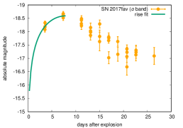
The rise time and peak luminosity of our SN IIn sample are estimated using the method developed by Ofek et al. (2014a). We fit the rising part of the light-curves to estimate and ,
| (11) |
where is the time of the luminosity peak. The fits are shown in Fig. 3, and the estimated rise times and peak luminosities are summarized in Table 1. Because of the uncertainties in the rise time and the peak luminosity caused by the distance uncertainties and bolometric corrections, we assume a uncertainty of 3 days and 0.3 mag in the rise time and peak luminosity, respectively.
Table 1 also includes the CSM density estimates. We also show the corresponding mass-loss rates for . The estimated mass-loss rates with range from to , and they are consistent with previous studies (e.g., Ofek et al., 2014a; Moriya & Maeda, 2014). In the following analysis, we assume an 0.5 dex uncertainty in CSM density estimates to account for possible systematic uncertainties as well as the uncertainties in estimating rise time and peak luminosity.


5 Environmental dependence
Using the SN IIn environmental properties (Section 3) and SN IIn properties (Section 4), we next investigate if there exist any correlations among them. We evaluate the Pearson correlation coefficient to determine the existence and strength of correlations. We employ bootstrapping simulations and derive the Pearson correlation coefficient, its standard deviation, and the value for each. Each bootstrapping simulation is performed by randomly selecting 21 SNe allowing multiple selections of the same SN IIn.
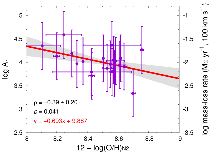
Table 4 summarizes the Pearson correlation coefficients, their standard deviations, and the values for each. One statistically significant correlation is a positive correlation between the peak magnitude and all three metallicity indicators. This means that more luminous SNe IIn tend to appear in lower metallicity environments. Figure 1 illustrates the correlation. The other significant correlation is a very weak positive correlation between the peak magnitude and the average light-weighted stellar population age (). In other words, more luminous SNe IIn prefer to occur in environments with younger stellar populations (Fig. 2). We also found that metallicity and average light-weighted stellar population age might be weakly correlated (Fig. 3). Thus, it is not clear if the peak luminosity correlation is driven by metallicity, stellar population age, or both. Because we found stronger correlations with metallicity, it is possible that metallicity difference is the main cause of the correlation.
It is worth noting that we do not find significant correlations between metallicity and CSM density (Fig. 4). A very weak negative correlation between metallicity and CSM density (i.e., SNe IIn with higher metallicity tend to have less dense CSM) may exist, but it is still statistically marginal and depends on the metallicity indicator. Interestingly, no positive correlation is likely to exist. Taddia et al. (2015) previously investigated the metallicity dependence of mass-loss rates and wind velocities in SNe IIn. They concluded that SNe IIn from higher metallicity environments have higher mass-loss rates and wind velocities. Figure 5 shows the CSM density estimates from the SNe IIn used in their analysis. The mass-loss rates and wind velocities in Taddia et al. (2015) estimates taken from a range of sources using different methodologies, and are not necessarily estimated in a consistent way. Nonetheless, we do not find a significant correlation in the CSM density and metallicity in their sample, either. Our results show that, although mass-loss rates and wind velocities may have metallicity dependence as proposed by Taddia et al. (2015), the CSM density () is not significantly metallicity dependent.
For the other combinations of the parameters, we do not find any statistically significant correlations. There may be other very weak correlations such as between the rise time and , between the peak magnitude and , and between and . More SNe IIn are required to determine the validity of any additional correlations.


6 Discussion
We found that there is a negative correlation between metallicity and peak luminosity of SNe IIn in the sense that more luminous SNe IIn are associated with lower metallicity environments. We also found a weak negative correlation between stellar population age and peak luminosity. The luminosity of SNe IIn can be characterized by , where is the kinetic energy in the shocked SN ejecta up to the time of the luminosity peak (Moriya & Maeda, 2014). We found that rise time, which is related to , does not correlate with metallicity or stellar age. The conversion efficiency is not likely to be sensitive to metallicity and stellar population age, although it could be higher for higher metallicities because of more efficient cooling. Thus, the negative correlation could be caused by the fact that SNe IIn tend to have higher explosion energy at lower metallicity environments and/or younger stellar populations. Because higher mass progenitors tend to have higher explosion energies (e.g., Martinez et al., 2022), it may be natural to expect that SNe IIn from younger stellar populations to have higher explosion energies. However, we do not find any correlations between EW(H) and peak luminosity. It is also possible that SN IIn progenitor masses tend to be higher at lower metallicity.
We did not find a significant correlation between metallicity and CSM density. This is interesting because some mass-loss mechanisms predict a positive correlation between mass-loss rate and metallicity. For example, in the case of hot massive stars, Björklund et al. (2021) find that
| (12) |
with and . Here, is metallicity and is luminosity of a star. This leads to a CSM density factor scaling of
| (13) |
For a given luminosity, the CSM density is expected to positively correlate with the metallicity. In order to have no or negative correlations between and , the SN IIn progenitor luminosity could increase at low metallicity. Ignoring the small term and assuming for SN IIn progenitors, we obtain . Thus, is required to have no or negative correlations between and . If the progenitor luminosity is close to the Eddington luminosity (i.e., ), an increase in progenitor mass by a factor of around 2 for a metallicity increase by a factor of 0.3 would produce no correlations, for example.
In the case of cool stars such as RSGs, the metallicity dependence of is not so clear. RSG mass-loss rates have been suggested to follow a relation of with (Mauron & Josselin, 2011, and the references therein), while Goldman et al. (2017) suggested no metallicity dependence for RSG mass-loss rates ( with ). The two prescriptions predict quite different CSM density dependences on metallicity with (Mauron & Josselin, 2011) or (Goldman et al., 2017). In both cases, CSM density around RSGs is predicted to strongly depend on metallicity. Nonetheless, because of huge uncertainties in the metallicity dependence of RSG mass loss, it is difficult to judge from the metallicity dependence whether SN IIn progenitors are dominated by RSGs or not. Additional investigations into the metallicity dependence of RSG mass loss are required.
Because of their high mass-loss rates, the progenitors of SNe IIn may actually have optically-thick winds forming a dense CSM. Mass-loss rates and wind velocities from optically-thick winds are also predicted to be metallicity dependent, but their dependence may also compensate to have a metallicity-independent CSM density (e.g., Gräfener & Hamann, 2008; Sander et al., 2020).
It is also possible that the normal mass-loss mechanisms for hot and cool stars are irrelevant for SN IIn progenitors. Their CSM density may be driven by a totally different mass-loss mechanism that is not strongly affected by metallicity. Precursors observed in some SNe IIn (e.g., Ofek et al., 2013; Strotjohann et al., 2021) may indeed indicate that their mass-loss mechanism is quite different from those of metallicity-dependent steady winds discussed above. For example, continuum-driven winds are not expected to have a metallicity dependence (e.g., Smith & Owocki, 2006). Further investigation of the environmental dependence of SN IIn properties would help understanding such an unknown mass-loss mechanism in SNe IIn.
Another possibility to explain the apparent lack of a metallicity dependence is that the CSM density actually depends on the metallicity, but we do not find it clearly because the CSM density needs to be high enough to be observed as SNe IIn. We might be simply biased to SNe having a CSM density above a certain metallicity-independent threshold by observing SNe IIn. In such a case, the apparent lack of the metallicity dependence would simply be an observational bias.
7 Conclusions
Using 21 SNe IIn with good light-curves and local IFS data, we investigated the relationship between local environments and SN properties. We found that SNe IIn with a higher peak luminosity tend to be in environments with lower metallicities and stellar population ages. Because metallicity and stellar population age are correlated in our sample, it is unclear if metallicity, stellar population age, or both drive the correlations. The correlations may indicate that SNe IIn have higher explosion energies in environments with lower metallicity and/or younger stellar ages.
We did not find statistically significant correlations between local metallicity and CSM density around SNe IIn. There might be a very weak negative correlation, but no positive correlation exists. This indicates that the mass-loss mechanism triggering the formation of dense CSM around SNe IIn could be metallicity independent. Alternatively, SN IIn progenitor mass range may depend on metallicity. It is also possible that the lack of the metallicity dependence is an observational bias due to needing a minimum threshold CSM density to be classified as a SN IIn.
Our study is based on 21 SNe IIn. Some correlations are still not significant and further confirmation is required. In addition, it is possible that some bias exist in our samples. Thus, a similar study with larger numbers of SNe IIn is encouraged. Wide-field high-cadence transient surveys are increasing the number of well-observed SNe IIn. Follow-up observations to obtain local environment information to increase the sample size will be important in uncovering the mysterious nature of SNe IIn.
Acknowledgements.
We thank the anonymous referee for thoughtful comments. This work was supported by the NAOJ Research Coordination Committee, NINS (NAOJ-RCC-2201-0401). TJM is supported by the Grants-in-Aid for Scientific Research of the Japan Society for the Promotion of Science (JP20H00174, JP21K13966, JP21H04997). L.G. acknowledges financial support from the Spanish Ministerio de Ciencia e Innovación (MCIN), the Agencia Estatal de Investigación (AEI) 10.13039/501100011033, and the European Social Fund (ESF) ”Investing in your future” under the 2019 Ramón y Cajal program RYC2019-027683-I and the PID2020-115253GA-I00 HOSTFLOWS project, from Centro Superior de Investigaciones Científicas (CSIC) under the PIE project 20215AT016, and the program Unidad de Excelencia María de Maeztu CEX2020-001058-M. H.K. was funded by the Academy of Finland projects 324504 and 328898. JDL acknowledges support from a UK Research and Innovation Fellowship (MR/T020784/1). We acknowledge the Telescope Access Program (TAP) funded by the NAOC, CAS and the Special Fund for Astronomy from the Ministry of Finance. SD acknowledges Project number 12133005 supported by National Natural Science Foundation of China (NSFC) and the Xplorer Prize. This work is supported by the Japan Society for the Promotion of Science Open Partnership Bilateral Joint Research Project between Japan and Chile (JPJSBP120209937, JPJSBP120239901). This work was funded by ANID, Millennium Science Initiative, ICN12_009. Based on observations collected at the Centro Astronómico Hispano en Andalucía (CAHA) at Calar Alto, operated jointly by Junta de Andalucía and Consejo Superior de Investigaciones Científicas (IAA-CSIC). Based on observations collected at the European Organisation for Astronomical Research in the Southern Hemisphere under ESO programmes 096.D-0296, 0100.D-0341, 0103.D-0440, 0101.D-0748, 196.B-0578, and 1100.B-0651. This research was partly supported by the Munich Institute for Astro-, Particle and BioPhysics (MIAPbP) which is funded by the Deutsche Forschungsgemeinschaft (DFG, German Research Foundation) under Germany´s Excellence Strategy – EXC-2094 – 390783311.Appendix A Figures of the SN environments
We present supplementary figures presenting each SN environment. Figure 6 shows SN host galaxies with SN locations, and Fig. 7 shows their spectra used for SN environment parameter estimations.


Appendix B Light-curve fitting results
The results of light-curve fitting that are used to estimate rise time and peak luminosity of our SN IIn sample are presented in Fig. 3. The fitting formula is Eq. (11).


References
- Anderson et al. (2015) Anderson, J. P., James, P. A., Habergham, S. M., Galbany, L., & Kuncarayakti, H. 2015, PASA, 32, e019
- Bacon et al. (2014) Bacon, R., Vernet, J., Borisova, E., et al. 2014, The Messenger, 157, 13
- Barbarino et al. (2017) Barbarino, C., Nyholm, A., Taddia, F., et al. 2017, Transient Name Server Classification Report, 2017-293, 1
- Björklund et al. (2021) Björklund, R., Sundqvist, J. O., Puls, J., & Najarro, F. 2021, A&A, 648, A36
- Blanton et al. (2017) Blanton, M. R., Bershady, M. A., Abolfathi, B., et al. 2017, AJ, 154, 28
- Brimacombe et al. (2016a) Brimacombe, J., Brown, J. S., Stanek, K. Z., et al. 2016a, The Astronomer’s Telegram, 9344, 1
- Brimacombe et al. (2016b) Brimacombe, J., Brown, J. S., Stanek, K. Z., et al. 2016b, The Astronomer’s Telegram, 9439, 1
- Brimacombe et al. (2016c) Brimacombe, J., Kiyota, S., Holoien, T. W. S., et al. 2016c, The Astronomer’s Telegram, 8703, 1
- Brown et al. (2016) Brown, J. S., Prieto, J. L., Shappee, B. J., et al. 2016, The Astronomer’s Telegram, 9445, 1
- Bundy et al. (2015) Bundy, K., Bershady, M. A., Law, D. R., et al. 2015, ApJ, 798, 7
- Chandra et al. (2022) Chandra, P., Chevalier, R. A., James, N. J. H., & Fox, O. D. 2022, MNRAS, 517, 4151
- Chen et al. (2022) Chen, P., Dong, S., Kochanek, C. S., et al. 2022, ApJS, 259, 53
- Chevalier & Fransson (2006) Chevalier, R. A. & Fransson, C. 2006, ApJ, 651, 381
- Cid Fernandes et al. (2005) Cid Fernandes, R., Mateus, A., Sodré, L., Stasińska, G., & Gomes, J. M. 2005, MNRAS, 358, 363
- Cid Fernandes et al. (2009) Cid Fernandes, R., Schoenell, W., Gomes, J. M., et al. 2009, in Revista Mexicana de Astronomia y Astrofisica Conference Series, Vol. 35, Revista Mexicana de Astronomia y Astrofisica Conference Series, 127–132
- Dong et al. (2015) Dong, S., Davis, A. B., Holoien, T. W. S., et al. 2015, The Astronomer’s Telegram, 6864, 1
- Dopita et al. (2016) Dopita, M. A., Kewley, L. J., Sutherland, R. S., & Nicholls, D. C. 2016, Ap&SS, 361, 61
- Elias-Rosa et al. (2016) Elias-Rosa, N., Kromer, M., Faran, T., et al. 2016, The Astronomer’s Telegram, 8727, 1
- Filippenko (1997) Filippenko, A. V. 1997, ARA&A, 35, 309
- Fitzpatrick (1999) Fitzpatrick, E. L. 1999, PASP, 111, 63
- Fransson et al. (2014) Fransson, C., Ergon, M., Challis, P. J., et al. 2014, ApJ, 797, 118
- Gal-Yam & Leonard (2009) Gal-Yam, A. & Leonard, D. C. 2009, Nature, 458, 865
- Galbany et al. (2016a) Galbany, L., Anderson, J. P., Rosales-Ortega, F. F., et al. 2016a, MNRAS, 455, 4087
- Galbany et al. (2018) Galbany, L., Anderson, J. P., Sánchez, S. F., et al. 2018, ApJ, 855, 107
- Galbany et al. (2014) Galbany, L., Stanishev, V., Mourão, A. M., et al. 2014, A&A, 572, A38
- Galbany et al. (2016b) Galbany, L., Stanishev, V., Mourão, A. M., et al. 2016b, A&A, 591, A48
- Goldman et al. (2017) Goldman, S. R., van Loon, J. T., Zijlstra, A. A., et al. 2017, MNRAS, 465, 403
- Gräfener & Hamann (2008) Gräfener, G. & Hamann, W. R. 2008, A&A, 482, 945
- Habergham et al. (2014) Habergham, S. M., Anderson, J. P., James, P. A., & Lyman, J. D. 2014, MNRAS, 441, 2230
- Hicken et al. (2017) Hicken, M., Friedman, A. S., Blondin, S., et al. 2017, ApJS, 233, 6
- Hinshaw et al. (2013) Hinshaw, G., Larson, D., Komatsu, E., et al. 2013, ApJS, 208, 19
- Kelz et al. (2006) Kelz, A., Verheijen, M. A. W., Roth, M. M., et al. 2006, PASP, 118, 129
- Kennicutt (1998) Kennicutt, Robert C., J. 1998, ApJ, 498, 541
- Kiewe et al. (2012) Kiewe, M., Gal-Yam, A., Arcavi, I., et al. 2012, ApJ, 744, 10
- Kochanek et al. (2017) Kochanek, C. S., Shappee, B. J., Stanek, K. Z., et al. 2017, PASP, 129, 104502
- Kumar et al. (2019) Kumar, B., Eswaraiah, C., Singh, A., et al. 2019, MNRAS, 488, 3089
- Kuncarayakti et al. (2018) Kuncarayakti, H., Anderson, J. P., Galbany, L., et al. 2018, A&A, 613, A35
- Kuncarayakti et al. (2016) Kuncarayakti, H., Galbany, L., Anderson, J. P., Krühler, T., & Hamuy, M. 2016, A&A, 593, A78
- Li et al. (2011) Li, W., Chornock, R., Leaman, J., et al. 2011, MNRAS, 412, 1473
- López-Cobá et al. (2020) López-Cobá, C., Sánchez, S. F., Anderson, J. P., et al. 2020, AJ, 159, 167
- Lyman et al. (2017) Lyman, J., Homan, D., & Yaron, O. 2017, Transient Name Server Classification Report, 2017-937, 1
- Marino et al. (2013) Marino, R. A., Rosales-Ortega, F. F., Sánchez, S. F., et al. 2013, A&A, 559, A114
- Martinez et al. (2022) Martinez, L., Anderson, J. P., Bersten, M. C., et al. 2022, A&A, 660, A42
- Matzner & McKee (1999) Matzner, C. D. & McKee, C. F. 1999, ApJ, 510, 379
- Mauron & Josselin (2011) Mauron, N. & Josselin, E. 2011, A&A, 526, A156
- Moller et al. (2017) Moller, A., Tucker, B., Zhang, B., et al. 2017, Transient Name Server Discovery Report, 2017-923, 1
- Moran et al. (2023) Moran, S., Fraser, M., Kotak, R., et al. 2023, A&A, 669, A51
- Moriya & Maeda (2014) Moriya, T. J. & Maeda, K. 2014, ApJ, 790, L16
- Moriya et al. (2014) Moriya, T. J., Maeda, K., Taddia, F., et al. 2014, MNRAS, 439, 2917
- Nyholm et al. (2020) Nyholm, A., Sollerman, J., Tartaglia, L., et al. 2020, A&A, 637, A73
- Ofek et al. (2014a) Ofek, E. O., Arcavi, I., Tal, D., et al. 2014a, ApJ, 788, 154
- Ofek et al. (2010) Ofek, E. O., Rabinak, I., Neill, J. D., et al. 2010, ApJ, 724, 1396
- Ofek et al. (2013) Ofek, E. O., Sullivan, M., Cenko, S. B., et al. 2013, Nature, 494, 65
- Ofek et al. (2014b) Ofek, E. O., Zoglauer, A., Boggs, S. E., et al. 2014b, ApJ, 781, 42
- Onori et al. (2017) Onori, F., Hamanowicz, A., Fraser, M., & Yaron, O. 2017, Transient Name Server Classification Report, 2017-354, 1
- Osterbrock & Ferland (2006) Osterbrock, D. E. & Ferland, G. J. 2006, Astrophysics of gaseous nebulae and active galactic nuclei
- Pan (2017) Pan, Y. 2017, Transient Name Server Classification Report, 2017-745, 1
- Pastorello et al. (2018) Pastorello, A., Kochanek, C. S., Fraser, M., et al. 2018, MNRAS, 474, 197
- Pessi et al. (2021) Pessi, P., Csoernyei, G., Holas, A., et al. 2021, Transient Name Server AstroNote, 118, 1
- Pettini & Pagel (2004) Pettini, M. & Pagel, B. E. J. 2004, MNRAS, 348, L59
- Poon et al. (2011) Poon, H., Pun, J. C. S., Lam, T. Y., Qiu, Y. L., & Wei, J. Y. 2011, arXiv e-prints, arXiv:1109.0899
- Prieto et al. (2008) Prieto, J. L., Kistler, M. D., Thompson, T. A., et al. 2008, ApJ, 681, L9
- Ransome et al. (2022) Ransome, C. L., Habergham-Mawson, S. M., Darnley, M. J., James, P. A., & Percival, S. M. 2022, MNRAS, 513, 3564
- Reynolds et al. (2016) Reynolds, T., Fraser, M., & Yaron, O. 2016, Transient Name Server Classification Report, 2016-544, 1
- Roth et al. (2005) Roth, M. M., Kelz, A., Fechner, T., et al. 2005, PASP, 117, 620
- Sánchez et al. (2016) Sánchez, S. F., García-Benito, R., Zibetti, S., et al. 2016, A&A, 594, A36
- Sánchez et al. (2015) Sánchez, S. F., Pérez, E., Rosales-Ortega, F. F., et al. 2015, A&A, 574, A47
- Sander et al. (2020) Sander, A. A. C., Vink, J. S., & Hamann, W. R. 2020, MNRAS, 491, 4406
- Schlegel (1990) Schlegel, E. M. 1990, MNRAS, 244, 269
- Shappee et al. (2014) Shappee, B. J., Prieto, J. L., Grupe, D., et al. 2014, ApJ, 788, 48
- Shappee et al. (2015) Shappee, B. J., Prieto, J. L., Holoien, T. W. S., et al. 2015, The Astronomer’s Telegram, 6882, 1
- Sharma et al. (2023) Sharma, Y., Sollerman, J., Fremling, C., et al. 2023, arXiv e-prints, arXiv:2301.04637
- Smith (2014) Smith, N. 2014, ARA&A, 52, 487
- Smith & Andrews (2020) Smith, N. & Andrews, J. E. 2020, MNRAS, 499, 3544
- Smith & Owocki (2006) Smith, N. & Owocki, S. P. 2006, ApJ, 645, L45
- Sorce et al. (2014) Sorce, J. G., Tully, R. B., Courtois, H. M., et al. 2014, MNRAS, 444, 527
- Springob et al. (2014) Springob, C. M., Magoulas, C., Colless, M., et al. 2014, MNRAS, 445, 2677
- Strotjohann et al. (2021) Strotjohann, N. L., Ofek, E. O., Gal-Yam, A., et al. 2021, ApJ, 907, 99
- Taddia et al. (2015) Taddia, F., Sollerman, J., Fremling, C., et al. 2015, A&A, 580, A131
- Taddia et al. (2013) Taddia, F., Stritzinger, M. D., Sollerman, J., et al. 2013, A&A, 555, A10
- Takats et al. (2016) Takats, K., Rodriguez, O., Galbany, L., & Yaron, O. 2016, Transient Name Server Classification Report, 2016-932, 1
- Theureau et al. (2007) Theureau, G., Hanski, M. O., Coudreau, N., Hallet, N., & Martin, J. M. 2007, A&A, 465, 71
- Tonry et al. (2021) Tonry, J., Denneau, L., Heinze, A., et al. 2021, Transient Name Server Discovery Report, 2021-771, 1
- Tonry et al. (2016) Tonry, J., Denneau, L., Stalder, B., et al. 2016, Transient Name Server Discovery Report, 2016-909, 1
- Tonry et al. (2017a) Tonry, J., Stalder, B., Denneau, L., et al. 2017a, Transient Name Server Discovery Report, 2017-284, 1
- Tonry et al. (2017b) Tonry, J., Stalder, B., Denneau, L., et al. 2017b, Transient Name Server Discovery Report, 2017-336, 1
- Tonry et al. (2017c) Tonry, J., Stalder, B., Denneau, L., et al. 2017c, Transient Name Server Discovery Report, 2017-709, 1
- Tsuna et al. (2019) Tsuna, D., Kashiyama, K., & Shigeyama, T. 2019, ApJ, 884, 87
- Tully et al. (2013) Tully, R. B., Courtois, H. M., Dolphin, A. E., et al. 2013, AJ, 146, 86
- Van Dyk et al. (2000) Van Dyk, S. D., Peng, C. Y., King, J. Y., et al. 2000, PASP, 112, 1532
- Verheijen et al. (2004) Verheijen, M. A. W., Bershady, M. A., Andersen, D. R., et al. 2004, Astronomische Nachrichten, 325, 151
- Weis & Bomans (2020) Weis, K. & Bomans, D. J. 2020, Galaxies, 8, 20
- Willick & Batra (2001) Willick, J. A. & Batra, P. 2001, ApJ, 548, 564
- Xu et al. (2017) Xu, Z., Li, B., Li, Z., et al. 2017, Transient Name Server Discovery Report, 2017-903, 1