Environment-stored memory in active nematics and extra-cellular matrix remodeling

Active nematics are systems composed of self-propelling constituents capable of aligning along a shared axis with no preferred overall direction . The active isotropic-nematic transition has been studied extensively [1, 2, 3, 4]. Similar to passive liquid crystals, order is driven by strong aligning fields, obtained by a combination of strong interactions and high densities. Unlike passive systems, activity couples order with propulsion and allows for coexistence between a dilute isotropic phase and dense nematic phase.

Active nematics are ubiquitous in biological systems at different scales. Our main motivation is cells in extra-cellular matrix (ECM), which are both capable of displaying nematic order. Growing biological evidence suggests that the interplay between cellular and ECM order is essential for tissue patterning and multicellular migration [5, 6, 7, 8, 9]. In particular, aligned collagen structures have been shown to greatly promote metastasis [10, 11].

Cell-ECM coupling is especially evident in fibroblasts that deposit, degrade and re-arrange ECM fibers [12, 13]. This has been modeled in different contexts, including wound healing [14], fibroblast alignment [15], and ECM patterning [16, 8]. However, the macroscopic physical mechanisms underlying cell-environment interplay and their role in determining orientational order and dynamics are not well understood or quantified.

Our approach to understand cell-environment interplay is to consider them as a two-component active system. We recently applied such a description to explain mechanical feedback mechanisms between cells and ECM [17, 18]. Here we focus on chemical remodeling. We find that environment-stored memory acts as an external field that allows for steady-state nematic order at arbitrarily low densities and constrains angular dynamics. We relate our results to recent in-vitro experiments on fibroblasts [8, 9]. While we are motivated by cells in ECM, our findings are generic and imply that the understanding of standard active matter may not apply in a dynamic environment, highlighting the need for further investigation and adaptation of existing theories .

Theory. We consider active cells and passive environment (matrix) segments in two dimensions, each described by their position and orientation, $\boldsymbol{r}$ and $\boldsymbol{n}$ for the cells and $\boldsymbol{r}^{\prime}$ and $\boldsymbol{n}^{\prime}$ for the matrix. Cells self-propel with a velocity $\boldsymbol{v}=v\boldsymbol{n}$ and diffuse with a diffusion coefficient $D$. They also align with neighboring cells and matrix segments. Matrix segments are considered to be apolar. They are enslaved to the cells that may deposit and degrade them (for more general choices, see SM in [19]) . These dynamics are described by the following equations:

where $\partial_{t}$ denotes the partial time derivative. The function $f_{\mathrm{c}}$ ($f_{\mathrm{m}}$) describes the distribution to find a cell (matrix segment) at position $\boldsymbol{r}$ ($\boldsymbol{r}^{\prime}$) with orientation $\boldsymbol{n}$ ($\boldsymbol{n}^{\prime}$). They are normalized such that $\int\mathrm{d}\boldsymbol{n}f_{\mathrm{c}}=\rho_{\mathrm{c}}$ is the cellular density and $\int\mathrm{d}\boldsymbol{n}^{\prime}f_{\mathrm{m}}=\rho_{\mathrm{m}}$ is the matrix density.

The cellular orientation dynamics are written in terms of a tumbling rate $k$, and an orientation probability, given by the Boltzmann factor $\exp\left(-E_{\mathrm{c}}\right)/Z_{\mathrm{c}}$ with the effective alignment energy $E_{\mathrm{c}}$ and partition function $Z_{\mathrm{c}}=\int\mathrm{d}\boldsymbol{n}\exp\left(-E_{\mathrm{c}}\right)$ [20]. This is a convenient choice that allows for the recovery of passive systems in simple limits.

Matrix deposition and degradation are described by the rates $k_{+}\rho_{\mathrm{c}}$ and $k_{-}\rho_{\mathrm{c}}$, respectively. Here we assume that cells locally deposit segments along their axis of motion and degrade segments in all orientations. Similar ingredients of cell and matrix dynamics were recently proposed as part of a two-layer Viscek model [8]. We note that Eq. (Environment-stored memory in active nematics and extra-cellular matrix remodeling ) is written within mean field.

Averaging the different moments of the orientation angles yield mesoscopic fields that are the focus of our theory. The active cellular current density is given by $\boldsymbol{j}=v\int\mathrm{d}\boldsymbol{n}f_{\mathrm{c}}$, the cellular nematic tensor density is $\boldsymbol{Q}_{\mathrm{c}}=\int\mathrm{d}\boldsymbol{n}\,\left(\boldsymbol{n}\boldsymbol{n}-\boldsymbol{I}/2\right)f_{\mathrm{c}}$, and the matrix nematic tensor density is $\boldsymbol{Q}_{\mathrm{m}}=\int\mathrm{d}\boldsymbol{n}^{\prime}\,\left(\boldsymbol{n}^{\prime}\boldsymbol{n}^{\prime}-\boldsymbol{I}/2\right)f_{\mathrm{m}}.$ These fields are all extensive in the number of cells/matrix segments.

We coarse-grain Eq. (Environment-stored memory in active nematics and extra-cellular matrix remodeling ) into equations in terms of the average fields, using an approximation that neglects higher moments of $f_{\mathrm{c}}$ in $\boldsymbol{n}$ beyond the nematic tensor . In particular, we treat the orientation within mean field in terms of the interaction $E_{\mathrm{c}}\left(\boldsymbol{n}\right)=-2\text{Tr}\left[\left(\boldsymbol{n}\boldsymbol{n}-\boldsymbol{I}/2\right)\boldsymbol{Q}_{t}\right]$ with the total aligning field $\boldsymbol{Q}_{t}=\beta_{\mathrm{c}}\boldsymbol{Q}_{\mathrm{c}}+\beta_{\mathrm{m}}\boldsymbol{Q}_{\mathrm{m}}$. It includes cell-cell and cell-matrix alignment, with the interaction strengths $\beta_{\mathrm{c}}$ and $\beta_{\mathrm{m}}$, respectively (more general choices are given in the SM [19]). In the absence of cell activity and cell-matrix interaction, our choice of $E_{\mathrm{c}}$ leads to an equivalent of Maier-Saupe theory [21] for compressible two-dimensional systems.

The resulting field equations are [19]:

The first equation is the cellular continuity equation, given by the active cellular current $\boldsymbol{j}$ and passive diffusive current. The second equation is a polarization-rate equation for the active current, which we interpret below, at steady state, as a force balance equation.

The equation for $\boldsymbol{Q}_{\mathrm{c}}$ includes diffusion and shear-alignment (first line), as well as non-linear alignment terms that dominate at large lengthscales (second line). They are written in terms of the function $g(x)=I_{1}(x)/I_{0}(x),$ where $I_{n}(x)$ is the modified Bessel function of the first kind [22], which results from an angular average of the Boltzmann factor $\exp\left(-E_{\mathrm{c}}\right)$. The cellular dynamics include the first and second moments of the angular distribution ($\boldsymbol{j}$ and $\boldsymbol{Q}_{\mathrm{c}}$, respectively), similarly to “self-propelled rods” [23, 24, 25]. Finally, the matrix dynamics are governed by cellular deposition and degradation.

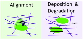
These equations define our framework for active nematics (cells) with environment-stored memory (matrix nematic order) , which we apply for the study of ECM remodeling. Cell-matrix interplay enters the theory in two ways: cellular alignment by the matrix as part of the nematic tensor $\boldsymbol{Q}_{t}$ and matrix remodeling by the cells (see Fig. 1). Cellular activity enters our theory in the active current $\boldsymbol{j}$, matrix deposition and degradation, and possibly in the alignment dynamics.

Next, we focus on the consequences of remodeling on the emergence of cellular and ECM orientational order at steady state as well as typical relaxation dynamics of the cell and matrix. For brevity, we rescale times with the run time $1/k$ and lengths with the typical cellular persistence length $v/k$, while keeping the same notation.

Results. The standard isotropic-nematic transition in active systems is similar to a gas-liquid transition [1, 26], where the alignment strength plays the role of inverse temperature. At low densities and high temperatures, the system forms a dilute isotropic gas, while at high densities and low temperatures - a nematic liquid. At intermediate densities and temperatures, the two phases co-exist and are generally linearly unstable. Here, we show how the matrix can break this behavior.

The key to understand the coexistence lies in the stress. In the hydrodynamic limit of large system size and long time, the total cellular current is proportional to a divergence of a tensor that we interpret as the stress  [19], $\boldsymbol{\sigma}=-\left[{\color[rgb]{0,0,0}\rho_{\mathrm{c}}}\boldsymbol{I}+2\boldsymbol{Q}_{\mathrm{c}}/\left(1+2D\right)\right]$. The steady-state behavior of the cells is thus described by a constant stress tensor. We consider a possible density profile along the $x$ direction and focus on the $xx$ component of the stress that we denote as $\sigma$ for brevity,

The first term is the ideal-gas contribution to the pressure, while the second term is an extensile active stress $\sim\boldsymbol{Q}_{\mathrm{c}}$ [27]. Here we consider ordering either along the $x$ axis ($Q_{\mathrm{c}}>0$) or the $y$ axis ($Q_{\mathrm{c}}<0$).

Co-existence is possible when the active stress decreases with density, compensating for the increase in ideal-gas pressure. This is the case for alignment in the $y$ direction. The stress $\sigma$ can be considered as a Lagrange multiplier that enforces the total number of cells. It is given by (minus) the density in the isotropic phase.

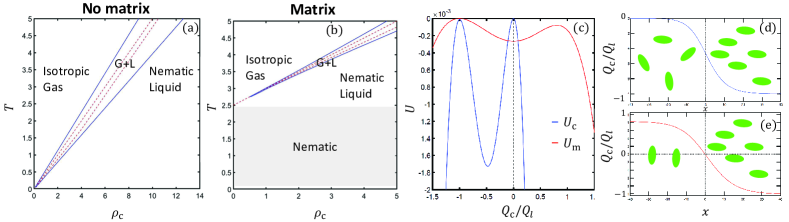
Next, we derive the isotropic-nematic phase diagram in the density-temperature plane, where $\beta_{\mathrm{c}},\beta_{\mathrm{m}}\sim 1/T$, and the ratio $\beta_{\mathrm{c}}/\beta_{\mathrm{m}}$ is kept fixed . Examples of such phase diagrams with and without a matrix (ECM) are given in Figs. 2a and 2b. The region of co-existence is delimited by the binodal line (solid blue line), within which lies a region of linear instability, delimited by the spinodal line (dashed red line).

Steady-state nematic order: matrix aligns cells at arbitrarily low densities. We solve Eq. (Environment-stored memory in active nematics and extra-cellular matrix remodeling ) at steady state. The matrix density is $\rho_{\mathrm{m}}=k_{+}/k_{-}$, independent of $\rho_{\mathrm{c}}$. The matrix nematic tensor has the same direction as the cellular one, chosen here as the $x$-axis. We define the intensive nematic order of the cells and matrix, $q_{\mathrm{c}}=Q_{\mathrm{c}}/\rho_{\mathrm{c}}$ and $q_{\mathrm{m}}=Q_{\mathrm{m}}/\rho_{\mathrm{m}}$, and find that $q_{\mathrm{m}}=q_{\mathrm{c}}$ at steady state.

The matrix thus inherits the same intensive nematic order as the cells. Consequently $Q_{t}=\left(\beta_{\mathrm{c}}\rho_{\mathrm{c}}+\beta_{\mathrm{m}}\rho_{\mathrm{m}}\right)q_{\mathrm{c}}$ at steady state, and the cellular nematic tensor solves

This is one of our main results. By expanding the right-hand-side of Eq. (4), we find that nematic order is possible for $\beta_{\mathrm{c}}\rho_{\mathrm{c}}+\beta_{\mathrm{m}}\rho_{\mathrm{m}}>2.$ The $\beta_{\mathrm{m}}\rho_{\mathrm{m}}$ term quantifies the matrix contribution and allows for nematic order even for vanishing cellular densities $\rho_{\mathrm{c}}\approx 0$ (grey region in Fig. 2b). The mechanism is simple: even dilute cells deposit a finite-density matrix after sufficiently long time. The matrix then acts as an external field that aligns the cells. Alternatively, rather than being aligned by current neighbors, cells are aligned by the memory of past neighbors, recorded by the matrix.

Next, we analyze the effect of ECM remodeling on the spinodal and binodal lines, as is plotted in Fig. 2.

Spinodal: matrix stabilizes the nematic order. The spinodal is given by $\partial\sigma/\partial\rho_{\mathrm{c}}=0$ for fixed values of $\beta_{\mathrm{c}}$ and $\beta_{\mathrm{m}}$ [19]. This threshold of linear instability is due to a negative compressibility. As the cellular density increases, the active stress overcomes the osmotic pressure and pushes cells up their concentration gradient. Note that active nematics can also be unstable due to a combination of active stress and shear alignment [28, 29], but this is not the case here, where the cells are effectively extensile and align with the strain rate.

Negative compressibility occurs for $\partial Q_{\mathrm{c}}/\partial\rho_{\mathrm{c}}<-\left(1+2D\right)$ [Eq. (3)]. In the isotropic state, $Q_{\mathrm{c}}\equiv 0$ and this is not possible. Deep in the ordered state, $Q_{\mathrm{c}}=\pm\rho_{\mathrm{c}}$, also ensuring stability. The instability is possible, therefore, only for intermediate $Q_{\mathrm{c}}$ values. For such values we expand the nonlinear terms of Eq. (4) and find its possible roots. One solution is $q_{\mathrm{c}}=0$ and the other is $q_{\mathrm{c}}=-\sqrt{\left(\beta_{\mathrm{m}}\rho_{\mathrm{m}}+\beta_{\mathrm{c}}\rho_{\mathrm{c}}-2\right)/\left(\beta_{\mathrm{m}}\rho_{\mathrm{m}}+\beta_{\mathrm{c}}\rho_{\mathrm{c}}\right)^{3}}.$

First, we examine the case of $\beta_{\mathrm{m}}\rho_{\mathrm{m}}<2.$ The cells are isotropic at low densities and become ordered at $\rho_{\ast}=\left(2-\beta_{\mathrm{m}}\rho_{\mathrm{m}}\right)/\beta_{\mathrm{c}}$. As $Q_{\mathrm{c}}\sim\sqrt{\rho-\rho_{\ast}}$ in this case, $\partial Q_{\mathrm{c}}/\partial\rho_{\mathrm{c}}\ll-1$ and the system is unstable. The cell density $\rho_{\ast}$ thus marks the gas spinodal line. Otherwise, for $\beta_{\mathrm{m}}\rho_{\mathrm{m}}>2$, the slope $\partial Q_{\mathrm{c}}/\partial\rho_{\mathrm{c}}$ at vanishing densities is given by $\sqrt{\left(\beta_{\mathrm{m}}\rho_{\mathrm{m}}-2\right)/\left(\beta_{\mathrm{m}}\rho_{\mathrm{m}}\right)^{3/2}}<1$. The matrix thus increases the compressibility and ensures stability. This is why the spinodal lies outside the grey region in Fig. 2b.

Binodal: matrix allows for co-existence between different orientations. The binodal describes, for a given temperature, the densities of the macroscopic phases at coexistence. We find it from the equation for $Q_{\mathrm{c}},$ while replacing $\rho_{\mathrm{c}}$ by its steady-state value, $-\sigma-Q_{\mathrm{c}}/\left(1+2D\right)$. Upon proper rescaling of lengths [19], we find that

This has the same structure as Newton’s equation, where $Q_{\mathrm{c}}$ plays the role of position and the $x$ coordinate - the role of time, while $F$ is the force (see also [30]). The first integral (conservation of energy) yields $E=Q_{\mathrm{c}}^{\prime 2}/2+U$, where we have denoted the “potential energy” $U=-\int\mathrm{d}Q_{\mathrm{c}}\,F\left(\sigma,Q_{\mathrm{c}}\right).$

Co-existence requires two $Q_{\mathrm{c}}$ values that have the same “potential energy” $U$. The co-existing phases can be either finite-sized or macroscopic, depending on the value of $F$. Macroscopic phases occur for $F=0$, where it takes an infinite “time” for the Newtonian particle to switch between the phases. These two conditions set $Q_{\mathrm{l}}$, the nematic order in the dense liquid phase, as well as $-\sigma=\rho_{\mathrm{g}}$, the density in the isotropic gas phase. To summarize, we require that $Q_{\mathrm{c}}=0,Q_{\mathrm{l}}$ are equally-valued maxima of $U$ at the binodal.

We highlight the effect of the environment by focusing on two limits: a cell-dominated interaction $U\left(\beta_{\mathrm{m}}=0\right)=U_{\mathrm{c}}$ where there is no matrix, and a matrix-dominated one $U\left(\beta_{\mathrm{c}}=0\right)=U_{\mathrm{m}}$, where the cells are aligned only by the matrix. Explicitly,

where $\tilde{\beta_{\mathrm{m}}}=\rho_{\mathrm{m}}\beta_{\mathrm{m}}.$ The difference between the two cases is the magnitude of the total nematic tensor ($Q_{t}$), which appears as the argument of the nonlinear $g$ function. In the cell-dominated case, the argument scales as the extensive $Q_{\mathrm{c}}$ that vanishes at small densities, while the matrix-dominated cases - as the intensive $q_{\mathrm{c}}$. The two potentials are plotted in Fig. 2c.

The intensive nematic order $q_{\mathrm{c}}$ in the cell-dominated case is a function of $\beta_{\mathrm{c}}\rho_{\mathrm{c}}$ [Eq. (4)] and both the spinodal and binodal lines are given by $\beta_{\mathrm{c}}\rho_{\mathrm{c}}=\mathrm{const,}$ as is displayed on Fig. 2a. In particular, we find that the nematic order at the liquid binodal $\beta_{\mathrm{c}}Q_{\mathrm{l}}$ is not necessarily small [19]. Therefore, we cannot find it from an expansion of $U_{\mathrm{c}}$, but rather from its full nonlinear form that we evaluate numerically (and see Fig. 2c) . We find that there is indeed a macroscopic coexistence between an isotropic gas and nematic liquid, obtained from the maxima of $U_{\mathrm{c}}$ for a specific value of $\rho_{\mathrm{g}}$. The value $\rho_{\mathrm{l}}$ is then found by requiring a fixed stress, i.e., $\rho_{\mathrm{g}}=\rho_{\mathrm{l}}+Q_{\mathrm{l}}/\left(1+2D\right)$. Co-existence was validated by numerical solutions of Eq. (Environment-stored memory in active nematics and extra-cellular matrix remodeling ) in 1D [31] , plotted in Fig. 2d.

The situation is very different in the matrix-dominated case. The value of $q_{\mathrm{c}}$ in this case depends only on $\tilde{\beta_{\mathrm{m}}}$ [Eq. (4)]. We expand for small $Q_{\mathrm{c}}$ and find $U_{\mathrm{m}}\sim-Q_{\mathrm{c}}^{2}\left[Q_{\mathrm{c}}^{2}-16\sigma^{2}\tilde{\beta_{\mathrm{m}}}^{-3}\left(-2+\tilde{\beta_{\mathrm{m}}}\right)\right]$. In this case, $Q_{\mathrm{c}}=0$ is a local minimum and the global maxima are $Q_{\mathrm{c}}=\pm 2\sigma\sqrt{\tilde{\beta_{\mathrm{m}}}^{-3}\left(-2+\tilde{\beta_{\mathrm{m}}}\right)}$.

Equation (4) ensures that for any solution $q_{\mathrm{c}}=q$ of $F=0,$ $q_{\mathrm{c}}=-q$ is also a solution. It can be shown analytically [19] that $q_{\mathrm{c}}<0$ is the global maximum, while $q_{\mathrm{c}}>0$ is a local one, as is demonstrated by a numerical plot of $U_{\mathrm{m}}$ in Fig. 2c. This form of $U_{\mathrm{m}}$ allows for co-existence between finite domains with nematic order in the $x$ and $y$ directions. For example, a nematic order $q_{\mathrm{c}}=q>0$, forced by surface anchoring, will transition to $q_{\mathrm{c}}=-q$ in the bulk, along a thickness that diverges logarithmically with $\tilde{\beta_{\mathrm{m}}}-2$ [19].

The co-existence between differently-oriented domains is verified by numerical solutions of Eq. (Environment-stored memory in active nematics and extra-cellular matrix remodeling ) in 1D [31], plotted in Fig. 2e. This new type of coexistence is possible because cells order at arbitrarily low densities. Then, cells aligned along the $x$ direction at very low densities can exert a positive active stress that matches $\sigma$. The exact form of co-existence profiles depends on angular dynamics, as explained next.

Angular dynamics: matrix possibly arrests domain coarsening. Finally, we focus on angular dynamics. While the system is invariant under global rotations of the cells and matrix together, their preferred mutual alignment results in a finite relaxation rate of their relative angle that is independent of system size. We define the angle between the preferred axis of the cells and the $x$ axis as $\phi_{\mathrm{c}}$ such that the two independent terms in $\boldsymbol{Q}_{\mathrm{c}}$ are $Q_{\mathrm{c}}\cos(2\phi_{\mathrm{c}})/2$ and $Q_{\mathrm{c}}\sin(2\phi_{\mathrm{c}})/2$. We similarly define $\phi_{\mathrm{m}}$ for the matrix . The relative angle between them is $\alpha/2=\phi_{\mathrm{c}}-\phi_{\mathrm{m}}$. We rewrite Eq. (Environment-stored memory in active nematics and extra-cellular matrix remodeling ) in terms of $Q_{\mathrm{c}}$, $Q_{\mathrm{m}}$, $\phi_{\mathrm{c}}$ and $\phi_{\mathrm{m}}$, and find that  [19].

where we have included the time scale $1/k$ explicitly. Note that all the densities and nematic orders also evolve in time and are coupled with $\alpha$, e.g., via shear alignment.

The two terms in the parenthesis on the right-hand side of Eq. (7) describe the dynamics of the cells and matrix, respectively. In the ordered state, their characteristic rates scale as $k\beta_{\mathrm{m}}\rho_{\mathrm{m}}/\left(\beta_{\mathrm{m}}\rho_{\mathrm{m}}+\beta_{\mathrm{c}}\rho_{\mathrm{c}}\right)$ and $k_{-}\rho_{\mathrm{c}},$ respectively [19]. The cellular rate depends on the typical cellular re-orientation rate and the strength of its alignment to the matrix field, while the matrix rate is defined by the degradation rate. The interplay between these two rates determines whether the cells are free to rotate with the matrix constantly remodeling according to the cells $[k_{-}\rho_{\mathrm{c}}\gg k\beta_{\mathrm{m}}\rho_{\mathrm{m}}/\left(\beta_{\mathrm{m}}\rho_{\mathrm{m}}+\beta_{\mathrm{c}}\rho_{\mathrm{c}}\right)]$ or the cells are pinned to the matrix $[k_{-}\rho_{\mathrm{c}}\ll k\beta_{\mathrm{m}}\rho_{\mathrm{m}}/\left(\beta_{\mathrm{m}}\rho_{\mathrm{m}}+\beta_{\mathrm{c}}\rho_{\mathrm{c}}\right)]$.

The latter implies that suppression of cellular relaxation dynamics. For example, consider ordered cellular domains of typical size $l$ with different orientations (different $\phi_{\mathrm{c}}$ values), such as alternating bands of width $l$ . As long as $k\beta_{\mathrm{m}}\rho_{\mathrm{m}}/\left(\beta_{\mathrm{m}}\rho_{\mathrm{m}}+\beta_{\mathrm{c}}\rho_{\mathrm{c}}\right)\gg D_{t}/l^{2},\,k_{-}\rho_{\mathrm{c}}$, we expect these domains to remain frozen, rather than relax into a common orientation, as is the usual case (see Supplemental Figure in [19]) . Here we have denoted $D_{t}$ as the total translational diffusion coefficient. In our model, it is given by $D_{t}=D+v^{2}/(4k)$.

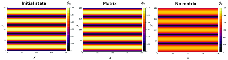
Discussion. This work demonstrates how environment-stored memory qualitatively changes the known behavior of active nematics. The underlying mechanism is generic: active particles generate a finite external field even for vanishing densities. Our findings open an avenue for novel behavior of active systems. Arrested domain coarsening, for example, suggests that the steady state may contain a signature of the initial conditions . Environment-induced relaxation dynamics should also slow down defect dynamics (as was shown very recently in  [32]) and possibly arrest typical instabilities, such as nematic bands at coexistence [1] and flow transitions [28]. Finally, this may also decrease the role of fluctuations beyond mean field .

Our finding are useful in understanding ECM remodeling by cells and its consequences on cellular and tissue dynamics. We focus on quasi-2D, in-vitro studies of fibroblasts and their derived matrices (see, e.g., Ref. [9].) The cells exchange momentum with the underlying substrate, as is the case in “dry” active systems. The rigid substrate also suppresses elastic matrix deformations. Nevertheless, ECM displays orientational order for cellular densities of the order $10^{-4}\mu\mathrm{m}^{-2}$, which correspond to $\rho_{\mathrm{c}}\approx 10^{-2}$, as can be understood from the memory effect in our theory (see also [15]). In setups where elasticity is important, it is expected to serve as another mechanism for alignment [33, 34]. Generally, ECM rheology is complex, including visco-plastic contributions [35].

It was recently reported [8] that fibroblast-ECM interaction promotes alignment in non-aligned ECMs, but may also decrease the range of alignment. This is explained by our theory in a simple way: increasing the interaction means a larger cellular aligning field $Q_{t}$, leading to alignment. At the same time, increasing $\beta_{\mathrm{m}}$ also increases the rate of cellular relaxation to the matrix, and may thus suppress domain coarsening. For dilute cells and assuming that the translational diffusion is mainly active ($D_{t}\sim v^{2}/k$), we predict a domain size of the order of the cellular persistence length, i.e., of the order $10\mu$m. This is consistent with experimental findings [9, 8]. In a future work, we will further apply our framework to predict ECM patterns observed in vivo.

In conclusion, our work demonstrates the profound effect of environment-stored memory on the steady-state and dyanmics of active nematics, especially in the biological context of ECM remodeling. It is generic in nature and is expected to play a similar role in additional active systems, including polar and synthetic.

Acknowledgements. We thank Erik Sahai and Raphaël Voituriez for useful discussions.

References

- Chaté [2020] H. Chaté, Dry aligning dilute active matter, Annual Review of Condensed Matter Physics 11, 189 (2020).
- Peshkov et al. [2012] A. Peshkov, I. S. Aranson, E. Bertin, H. Chaté, and F. Ginelli, Nonlinear field equations for aligning self-propelled rods, Physical review letters 109, 268701 (2012).
- Ngo et al. [2014] S. Ngo, A. Peshkov, I. S. Aranson, E. Bertin, F. Ginelli, and H. Chaté, Large-scale chaos and fluctuations in active nematics, Physical review letters 113, 038302 (2014).
- Großmann et al. [2016] R. Großmann, F. Peruani, and M. Bär, Mesoscale pattern formation of self-propelled rods with velocity reversal, Physical Review E 94, 050602 (2016).
- Clark and Vignjevic [2015] A. G. Clark and D. M. Vignjevic, Modes of cancer cell invasion and the role of the microenvironment, Current Opinion in Cell Biology 36, 13 (2015).
- Alexander and Cukierman [2016] J. Alexander and E. Cukierman, Stromal dynamic reciprocity in cancer: Intricacies of fibroblastic-ecm interactions, Current Opinion in Cell Biology 42, 80 (2016).
- Helvert et al. [2018] S. V. Helvert, C. Storm, and P. Friedl, Mechanoreciprocity in cell migration, Nature Cell Biology 20, 8 (2018).
- Wershof et al. [2019] E. Wershof, D. Park, R. P. Jenkins, D. J. Barry, E. Sahai, and P. A. Bates, Matrix feedback enables diverse higher-order patterning of the extracellular matrix, PLoS Computational Biology 15, 10.1371/journal.pcbi.1007251 (2019).
- Park et al. [2020] D. Park, E. Wershof, S. Boeing, A. Labernadie, R. P. Jenkins, S. George, X. Trepat, P. A. Bates, and E. Sahai, Extracellular matrix anisotropy is determined by tfap2c-dependent regulation of cell collisions, Nature Materials 19, 227 (2020).
- Conklin et al. [2011] M. W. Conklin, J. C. Eickhoff, K. M. Riching, C. A. Pehlke, K. W. Eliceiri, P. P. Provenzano, A. Friedl, and P. J. Keely, Aligned collagen is a prognostic signature for survival in human breast carcinoma, The American journal of pathology 178, 1221 (2011).
- Kopanska et al. [2016] K. S. Kopanska, Y. Alcheikh, R. Staneva, D. Vignjevic, and T. Betz, Tensile forces originating from cancer spheroids facilitate tumor invasion, PLoS One 11, e0156442 (2016).
- Phillips et al. [2009] R. Phillips, J. Kondev, J. Theriot, et al., Physical biology of the cell (Garland Science, 2009).
- Grinnell [2003] F. Grinnell, Fibroblast biology in three-dimensional collagen matrices, Trends in cell biology 13, 264 (2003).
- [14] L. Olsen, P. K. Mainia, J. A. Sherratt’, and B. Marchant, Simple modelling of extracellular matrix alignment in dermal wound healing i. cell flux induced alignment.
- Li et al. [2017] X. Li, R. Balagam, T.-F. He, P. P. Lee, O. A. Igoshin, and H. Levine, On the mechanism of long-range orientational order of fibroblasts, Proceedings of the National Academy of Sciences 114, 8974 (2017).
- Dallon et al. [1999] J. C. Dallon, J. A. Sherratt, and P. K. Maini, Mathematical modelling of extracellular matrix dynamics using discrete cells: Fiber orientation and tissue regeneration (1999).
- Adar and Joanny [2021] R. M. Adar and J. F. Joanny, Permeation instabilities in active polar gels, Physical Review Letters 127, 10.1103/PhysRevLett.127.188001 (2021).
- Adar and Joanny [2022] R. M. Adar and J.-F. Joanny, Active-gel theory for multicellular migration of polar cells in the extra-cellular matrix, New Journal of Physics 24, 073001 (2022).
- [19] See Supplemental Material at [URL will be inserted by publisher] for the derivation of Eqs. (Environment-stored memory in active nematics and extra-cellular matrix remodeling )-(7) and the details of the calculations presented in the Letter .
- [20] As cells are deformable and interact among themselves and with ECM via adhesion bonds, we describe the alignment via an interaction, . Generally, alignment can also be driven by excluded volume between hard rods.
- De Gennes and Prost [1993] P.-G. De Gennes and J. Prost, The physics of liquid crystals, 83 (Oxford university press, 1993).
- Abramowitz et al. [1988] M. Abramowitz, I. A. Stegun, and R. H. Romer, Handbook of mathematical functions with formulas, graphs, and mathematical tables (American Association of Physics Teachers, 1988).
- Marchetti et al. [2013] M. C. Marchetti, J. F. Joanny, S. Ramaswamy, T. B. Liverpool, J. Prost, M. Rao, and R. A. Simha, Hydrodynamics of soft active matter, Reviews of Modern Physics 85, 1143 (2013).
- Peruani et al. [2006] F. Peruani, A. Deutsch, and M. Bär, Nonequilibrium clustering of self-propelled rods, Physical Review E 74, 030904 (2006).
- Baskaran and Marchetti [2008] A. Baskaran and M. C. Marchetti, Enhanced diffusion and ordering of self-propelled rods, Physical Review Letters 101, 268101 (2008).
- Solon and Tailleur [2013] A. P. Solon and J. Tailleur, Revisiting the flocking transition using active spins, Physical review letters 111, 078101 (2013).
- [27] While our theory corresponds to an extensile active stress, cells such as fibroblasts are often contractile. The same qualitative results apply in the contractile case. The main difference is that the nematic order will form along the direction, rather than the direction.
- Voituriez et al. [2005] R. Voituriez, J.-F. Joanny, and J. Prost, Spontaneous flow transition in active polar gels, Europhysics Letters 70, 404 (2005).
- Duclos et al. [2018] G. Duclos, C. Blanch-Mercader, V. Yashunsky, G. Salbreux, J. F. Joanny, J. Prost, and P. Silberzan, Spontaneous shear flow in confined cellular nematics, Nature Physics 14, 728 (2018).
- Solon et al. [2015] A. P. Solon, J.-B. Caussin, D. Bartolo, H. Chaté, and J. Tailleur, Pattern formation in flocking models: A hydrodynamic description, Physical Review E 92, 062111 (2015).
- [31] Equation (2) was solved numerically in 1D using the “pdepe” function in Matlab with zero-flux boundary conditions. As an initial condition, we consider a homogeneous cellular density with and no matrix segments (), which are supplemented by small normally distributed fluctuations in and .
- Jacques et al. [2023] C. Jacques, J. Ackermann, S. Bell, C. Hallopeau, C. Perez-Gonzalez, L. Balasubramaniam, X. Trepat, B. Ladoux, A. Maitra, R. Voituriez, et al., Aging and freezing of active nematic dynamics of cancer-associated fibroblasts by fibronectin matrix remodeling, bioRxiv , 2023 (2023).
- De et al. [2007] R. De, A. Zemel, and S. A. Safran, Dynamics of cell orientation, Nature Physics 3, 655 (2007).
- Livne et al. [2014] A. Livne, E. Bouchbinder, and B. Geiger, Cell reorientation under cyclic stretching, Biophysical Journal 106, 42a (2014).
- Elosegui-Artola [2021] A. Elosegui-Artola, The extracellular matrix viscoelasticity as a regulator of cell and tissue dynamics, Current Opinion in Cell Biology 72, 10 (2021).
- You et al. [2020] Z. You, A. Baskaran, and M. C. Marchetti, Nonreciprocity as a generic route to traveling states, Proceedings of the National Academy of Sciences 117, 19767 (2020).
- Fruchart et al. [2021] M. Fruchart, R. Hanai, P. B. Littlewood, and V. Vitelli, Non-reciprocal phase transitions, Nature 592, 363 (2021).
Supplemental material for “Environment-stored memory in active nematics and extra-cellular matrix remodeling”
This Supplemental Material (SM) provides, in greater detail, the derivation of the hydrodynamic equations and phase diagram. The outline of the SM is as follows. In Sec. I, we coarse grain the microscopic dynamics [Eq. (1) of the Letter] into hydrodynamic equations [Eq. (2) of the Letter]. In Sec II, we solve the equations at steady-state, analyze the linear stability of the steady-state (spinodal) and derive the conditions for phase coexistence (binodal). Finally, in Sec. III, we derive the nonlinear equations for the angular dynamics.
I Derivation of hydrodynamic equations
As our starting point, we consider the following microscopic dynamics of the cells and matrix segments [Eq. (1) of the Letter],