P.O. Box 19395-5531, Tehran, Iran
Entropy of Hawking Radiation for Two-Sided Hyperscaling Violating Black Branes
Abstract
In this paper, we study the von Neumann entropy of Hawking radiation for a -dimensional Hyperscaling Violating (HV) black brane which is coupled to two Minkowski spacetimes as the thermal baths. We consider two different situations for the matter fields: First, they are described by a whose central charge is very large. Second, they are described by a d+2 dimensional HV QFT which has a holographic gravitational theory that is a HV geometry at zero temperature. For both cases, we calculate the Page curve of the Hawking radiation as well as the Page time . For the first case, grows linearly with time before the Page time and saturates after this time. Moreover, is proportional to , where and are the thermal entropy and temperature of the black brane. For the second case, when the hyperscaling violation exponent of the matter fields is zero, the results are very similar to those for the first case. However, when , the entropy of Hawking radiation grows exponentially before and saturates after this time. Furthermore, the Page time is proportional to , where is the renormalized Newton’s constant. It was also observed that for both cases, is a decreasing and an increasing function of the dynamical exponent and hyperscaling violation exponent of the black brane geometry, respectively. Moreover, for the second case, is independent of , and for , it is a decreasing function of .
Keywords:
AdS-CFT Correspondence, Gauge-gravity correspondenceIPM/P-2021/41
1 Introduction
It is well known that black holes can emit particles with a thermal spectrum which is called Hawking radiation Hawking:1975vcx . In this manner, a black hole loses its mass, and might be disappeared completely. Assuming that the black hole was formed from the collapse of some matter in a pure quantum state leads to the famous Hawking’s information paradox Hawking:1976ra , since the final state, i.e. the emitted radiation, is in a mixed state. Moreover, the final state cannot be obtained via a S matrix from the initial pure state. On the other hand, the fine-grained (von Neumann) entropy of the Hawking radiation grows linearly in time until the black hole completely disappears. In this manner, it eventually exceeds the coarse-grained (thermodynamic or Bekenstein-Hawking) entropy of the initial black hole. On the other hand, the von Neumann entropies of the black hole and radiation are equal to each other, i.e. , since the whole system is in a pure state. Moreover, the fine-grained entropy of the black hole has to be less than its coarse-grained entropy, i.e. Page:2013dx . Therefore, one has Page:2013dx (See also Almheiri:2020cfm )
| (1) |
The time at which the saturation happens is called the ”Page time” Page:1993wv ; Page:2013dx . Moreover, since the is a decreasing function of time, has to start decreasing after the Page time and goes to zero at the end of the evaporation. Consequently, the unitarity requires that the fine-grained entropy of Hawking radiation follows the so called Page curve Page:1993wv ; Page:2013dx .
Unearthing the unitary evaporation of Black holes is one of the most important puzzles in gravity. Recently, a very sophisticated resolution for information paradox which is called ”island rule” were introduced Penington:2019npb ; Almheiri:2019psf ; Almheiri:2019hni ; Almheiri:2019yqk in the context of the AdS/CFT correspondence Maldacena:1997re . This rule is inspired by the concept of ”Quantum Extremal Surfaces” (QES) Engelhardt:2014gca which are the generalization of the (H)RT surfaces Ryu:2006bv ; Hubeny:2007xt applied in the calculation of holographic entanglement entropy. More precisely, a QES is a classical spacelike codimension-two surface in the bulk spacetime which minimizes the generalized entropy Engelhardt:2014gca ; Faulkner:2013ana which is composed of an area term and the von Neumann entropy of matter quantum fields in a bulk region enclosed between the QES and the corresponding boundary region. The motivation for the island rule was the observation that the entanglement wedge (EW) of an evaporating black hole at late times does not include all of its interior. Therefore, one might naturally expects that the EW of the radiation region , which is a spatial region far away from the black hole where the radiation is collected, contains some parts of the black hole interior dubbed ”island” Penington:2019npb ; Almheiri:2019hni (See figure 1). Consequently, to calculate the von Neumann entropy of the Hawking radiation, one has to consider the contributions of islands.
According to the rule, one should first calculate the generalized entropy
as follows Almheiri:2019hni ; Almheiri:2019yqk
| (3) |
where is the boundary of the island and is a codimension-two surface. It is expected that for one-sided black holes is located inside the black hole Penington:2019npb ; Almheiri:2019psf ; Almheiri:2019hni ; Gautason:2020tmk ; Hartman:2020swn . However, for two-sided black holes, it is located outside the black hole Almheiri:2019yqk ; Almheiri:2019psy ; Gautason:2020tmk . If the matter quantum field theory has a gravitational dual theory, the island is connected to the radiation region through extra dimensions Almheiri:2019hni . Moreover, is the von Neumann entropy of matter quantum fields in the region . In the following, we denote the endpoints of and by and , respectively (See figure 1). Next, one has to extremize over all possible islands. If there is more than an island, one should consider the one which gives the minimum generalized entropy
| (4) |
In this case, is a minimal QES. Moreover, when there are no islands, the area term in eq. (3) vanishes, and hence the entropy of Hawking radiation is simply given by the von Neumann entropy of the matter fields on the region
| (5) |
The island rule were verified for two-dimensional Jackiw-Teitelboim (JT) black holes Jackiw:1984je ; Teitelboim:1983ux in refs. Penington:2019kki ; Almheiri:2019qdq ; Goto:2020wnk
222See also Marolf:2020rpm ; Bousso:2021sji for related discussions. Moreover, a new proof was recently introduced in ref. Pedraza:2021ssc which is based on minimizing the microcanonical action of an entanglement wedge.
by calculating the Euclidean gravitational path integral via replica trick in gravity Lewkowycz:2013nqa ; Dong:2016hjy . It was observed that the gravitational path integral has two saddle points: First, Hawking saddle which gives the usual entropy for Hawking radiation that grows linearly with time. Second, replica wormhole saddle which is a wormhole connecting various copies of the original black hole. It was observed that the replica saddle leads to the contribution of the islands and enforces the entropy of radiation to saturate. It should be pointed out that the Hawking saddle is dominant before the Page time. However, the replica wormhole saddle is dominant after the Page time.
Furthermore, the island rule have been explored extensively for various black holes in flat and AdS spacetimes such as:
JT gravity Penington:2019kki ; Almheiri:2019qdq ; Almheiri:2019yqk ; Hollowood:2020cou ; Chen:2020jvn ; Goto:2020wnk ; Chen:2019uhq ; Balasubramanian:2021xcm , two-dimensional dilaton gravity
Gautason:2020tmk ; Anegawa:2020ezn ; Hartman:2020swn ; Wang:2021mqq ; He:2021mst
, in higher dimensions Almheiri:2019psy ; Hashimoto:2020cas ; Karananas:2020fwx ; He:2021mst ; Chen:2020uac ; Chen:2020hmv ; Krishnan:2020fer ; Geng:2020qvw ; Matsuo:2020ypv ; Ghosh:2021axl ; Arefeva:2021kfx ; Saha:2021ohr , higher derivative gravity theories Alishahiha:2020qza , charged black holes Ling:2020laa ; Wang:2021woy ; Kim:2021gzd ; Ahn:2021chg ; Yu:2021cgi , pure BTZ black hole microstates
333These geometries are obtained by excising a two-sided BTZ black hole with a timelike dynamical brane, dubbed End-of-the-World (ETW) brane Kourkoulou:2017zaj ; Almheiri:2018ijj ; Cooper:2018cmb . The action-complexity of this model was studied in ref Omidi:2020oit .
Balasubramanian:2020hfs ; Anderson:2020vwi ; Fallows:2021sge , and black holes coupled to gravitating baths Balasubramanian:2021wgd ; Anderson:2020vwi ; Geng:2020fxl ; Geng:2021iyq . See also Almheiri:2020cfm for a very nice review on the topic.
Furthermore, the rule were applied
in de Sitter spacetime Hartman:2020khs ; Balasubramanian:2020xqf ; Aalsma:2021bit ; Sybesma:2020fxg ; Geng:2021wcq ; Chen:2020tes , flat-space cosmology
444It is a solution of the three dimensional Einstein gravity with no cosmological constant.
Azarnia:2021uch and separate universes Balasubramanian:2021wgd ; Balasubramanian:2020coy ; Miyata:2021ncm ; Fallows:2021sge ; Miyata:2021qsm .
In this paper, we study the von Neumann entropy of the Hawking radiation for a two-sided Hyperscaling Violating (HV) black brane which is coupled to two thermal baths that are Minkowski spacetimes. We assume that the matter fields in the black brane geometry as well as in the baths are described by the same QFT. We consider two different scenarios for the QFT: First, it is a d+2 dimensional CFT which does not necessarily have a dual gravity theory.
Second, it is a d+2 dimensional QFT which has a dual gravity theory that is a zero-temperature HV geometry (See eq. (88)). We dub it ”HV QFT”. We calculate for the two cases and verify that it obeys eq. (2). It is observed that at early times there are no islands. However, at late times there is an island which leads to the saturation of at twice the Bekenstein-Hawking entropy of the black brane. Moreover, we study the Page curve and Page time for different values of the dynamical exponent and hyperscaling violation exponent of the black brane. For the case where the matter is described by a HV QFT, we also study the behavior of the Page time and Page curve with respect to the dynamical and hyperscaling violation exponents of the HV QFT which are shown by and , respectively. We study the two cases and , separately.
The organization of the paper is as follows: in Section 2, we briefly review the HV black brane geometry. In Section 3, we calculate the entropy of Hawking radiation for the case where the matter fields
are described by a . We also find the Page time and study its behavior as a function of the dynamical exponent and hyperscaling violation exponent of the black brane geometry. In Section 4, we do the same calculations for the case where the matter fields are described by a d+2 dimensional HV QFT.
In section 5, we summarize our results and briefly address a few interesting future directions.
2 HV Black Branes
In this section, we briefly review Hyperscaling Violating (HV) black branes. These are solutions to the Einstein-Maxwell-Dilaton gravity with the following action Alishahiha:2012qu
| (6) |
The gauge field breaks Lorentz invariance and introduces the dynamical exponent . 555It should be pointed out that the action is Lorentz invariant and the solution does not respect the Lorentz symmetry. More precisely, under the coordinate transformation Dong:2012se the metric (11) is covariant, i.e. . It is clear that there is an anisotropy among the and coordinates in the above transformation. Therefore, the Lorentz symmetry is broken when , and it is a consequence of having a non-zero gauge field in eq. (9) for . Moreover, the non-trivial potential breaks the scaling symmetry and introduces the Hyperscaling Violation exponent . The dilaton field , its potential and the field strength of the gauge field are given by (See ref. Alishahiha:2012qu for more details)
| (7) | |||||
| (9) |
where the constant parameters are defined as follows
| (10) |
On the other hand, the metric of the black brane is given by Alishahiha:2012qu 666We set the AdS radius to one, i.e. . Moreover, we also set the dynamical scale to one.
| (11) |
where the emblankening factor is as follows
| (12) |
Here we defined and an effective dimension . Furthermore, the null energy condition puts the following constraints on the values of and
| (13) |
In the following, we restrict ourselves to the case and . 777As mentioned in ref. Alishahiha:2012qu , this solution is not valid for the case . Moreover, for the geometry is unstable Dong:2012se . It should also be pointed out that for and , the scaling and Lorentz symmetries are restored in the dual HV QFT. In this case, the scalar field becomes a constant and the gauge field equals to zero. Moreover, plays the rule of the cosmological constant , and hence the solution reduces to a d+2 dimensional AdS black brane. On the other hand, the temperature and thermal (Bekenstein-Hawking) entropy of the black brane are given by Alishahiha:2012qu
| (14) |
Here is the volume in the transverse directions . On the other hand, the tortoise coordinate is as follows
| (15) |
3 Entropy of Hawking Radiation: Matter CFT
In this section, we study the entropy of Hawking radiation for a two-sided HV black brane geometry. To allow the black brane to evaporate, we couple it to two thermal baths which are two Minkowski spacetimes on the left and right hand side of the Penrose diagram (See figure 1). Similar to ref. Almheiri:2019hni we add some matter fields in the bulk spacetime. For convenience, we assume that the matter fields in the HV black brane geometry and inside the two baths are described by the same QFT. Moreover, one can impose transparent boundary conditions Almheiri:2019qdq for the matter fields on the boundary of the HV black brane geometry. Furthermore, we assume that the matter fields are described by a . Then the whole action in the gravity region (see the purple region in figure 1) is given by
| (16) |
The CFT may Almheiri:2019hni ; Almheiri:2019psy ; Gautason:2020tmk ; Chen:2019uhq ; Chen:2020uac ; Chen:2020jvn ; Chen:2020hmv ; Ling:2020laa or may not Almheiri:2019yqk ; Alishahiha:2020qza ; Hashimoto:2020cas have a dual gravity theory. Moreover, we assume that its central charge is very large, i.e. . Therefore, the contributions of the matter fields of the to the EE are dominant over those of the graviton and the matter fields in Almheiri:2019hni ; Alishahiha:2020qza ; Azarnia:2021uch . Moreover, we assume that
| (17) |
to be able to neglect the backreaction of the matter on the HV black brane geometry Alishahiha:2020qza ; Azarnia:2021uch .
Furthermore, it is believed that the generalized entropy is finite and independent of the UV cutoff of the theory Bousso:2015mna ; Susskind:1994sm ; Engelhardt:2014gca ; Almheiri:2020cfm . On the other hand, there are some UV divergent terms in the entanglement entropy (EE) of a QFT, and the leading divergent term follows the area law Bombelli:1986rw ; Srednicki:1993im . Notice that our entangling regions are in the shape of strips on a constant time slice
such that they are extended in the transverse directions (See figure 1). Moreover, from holographic calculations, it is known that the EE of a strip with width and lengths in a holographic with which is in its vacuum state, is given by
Ryu:2006ef
888For spherical entangling regions there are subleading UV divergent terms Ryu:2006ef .
| (18) |
Here the first term is proportional to the area of the strip and the second term is a constant universal term. Inspired by this observation, one might expect that
| (19) |
where is the UV cutoff of the matter . Therefore, we renormalize Newton’s constant as follows Susskind:1994sm ; Almheiri:2020cfm ; Hashimoto:2020cas ; Alishahiha:2020qza ; Azarnia:2021uch 999It was shown in ref. Susskind:1994sm that in four dimensions, i.e. for d=2, the loop diagrams for matter fields lead to the renormalization of the gravitational coupling as in eq. (20). Moreover, this renormalization cancel the area law divergent term in eq. (19) such that the generalized entropy is finite. See Bousso:2015mna for a nice review on this topic.
| (20) |
to absorb the UV divergent term in eq. (19). Consequently, we merely consider the finite part of the EE of the matter fields in the following, and for an arbitrary interval in the bulk spacetime, we denote it by . Having said this, we rewrite the generalized entropy in eq. (3) as follows Hashimoto:2020cas ; Alishahiha:2020qza ; Azarnia:2021uch
| (21) |


Another important point is that the metric in eq. (11), has translational symmetries along the transverse directions . Therefore, one might expect that the locations of the endpoints of the island, and hence the generalized entropy are independent of the coordinates . Consequently, one might expect that the problem effectively reduces to two dimensions with coordinates . Moreover, by compactification of the directions, one might consider the transverse manifold which is parametrized by ’s, as a d dimensional sphere with a very large radius. In this manner, one might assume that the s-wave approximation mentioned in refs. Hashimoto:2020cas ; Alishahiha:2020qza ; He:2021mst ; Penington:2019npb can be applied. 101010We would like to thank Mohsen Alishahiha and Ali Naseh for their very helpful comments on this topic. In other words, after the expansion of the matter fields in terms of the spherical harmonics on the large sphere, one can have both massless and massive Kaluza-Klein modes. Then, each mode behaves as an independent free field in two dimensions (with coordinates and ) whose mass is proportional to the inverse of the radius of the sphere Penington:2019npb . Since the radius of the sphere is very large, the masses of the Kaluza-Klein modes have to be very small. Moreover, since the endpoints of the radiation region are very far from the endpoints of the islands 111111We are assuming that and , where and are the radial coordinates of the endpoints and , respectively. , we assume that only massless modes can reach the radiation region (See also Azarnia:2021uch ; Penington:2019npb ; Hashimoto:2020cas ). Therefore, the contribution of the massless modes to is dominant over that of the massive modes. 121212We would like to thank Ali Naseh for bringing this point to our attention. Consequently, one may apply the formula for a two dimensional CFT in its vacuum state to calculate , which for an interval of length is given by Holzhey:1994we ; Calabrese:2004eu
| (22) |
where is the central charge and is the UV cutoff.
3.1 Kruskal Coordinates and the Distances
For later convenience, it is better to work in the Kruskal coordinates. The advantage of working with the Kruskal coordinates is that the state on the whole Cauchy slice, i.e. the black brane plus the baths, is the vacuum state Almheiri:2019yqk ; He:2021mst , and hence one can simply apply the EE formula for the case where the matter QFT is in the vacuum state (See e.g. eq. (22)). For the black brane, they are defined as follows 131313Since the endpoints of the island are located outside the black brane horizon (See figure 1), we do not need the coordinates in the interior regions.
| (23) | |||||
| (25) |
where and is given by eq. (26). In the Kruskal coordinates, the metric of the black brane becomes
| (26) |
which is conformally flat in the and plane. Moreover, is the warp factor. On the other hand, for each of the two thermal baths which are Minkowski spacetimes, the tortoise coordinate is simply given by
| (27) |
On the other hand, one might consider the left and right baths as the Rindler wedges of a Minkowski spacetime Almheiri:2019yqk . In this manner, the Kruskal coordinates can be defined as follows for the two baths (See also refs. Almheiri:2019yqk ; Alishahiha:2020qza ; He:2021mst )
| (28) | |||||
| (30) |
Thus, the metric of each bath is given by (See also Azarnia:2021uch )
| (31) |
To calculate the entropy of Hawking radiation, one also needs to know the distances among the endpoints of the radiation region and island . We indicate the endpoints of the radiation region by and those of the island region by . From figure 1, one can easily find the coordinates of the endpoints as follows (See also Balasubramanian:2021xcm )
| (32) | |||
| (33) | |||
| (34) |
From eqs. (26) and (31), one can write the distance between two arbitrary points and in the bulk spacetime as follows
| (35) |
It is straightforward to verify that the distances are given by
| (36) | |||||
| (37) | |||||
| (39) | |||||
3.2 No Islands
When there are no islands, there are only the radiation regions (See the left panel of figure 1). In this case, the area term in eq. (3) vanishes, and hence the entropy of Hawking radiation is simply given by eq. (5). Therefore, one has
| (41) |
where is the EE of matter fields on the interval . In the last equality, we applied the fact that the whole state on the Cauchy slice is pure. Therefore, one can calculate the EE of matter fields on the interval instead of the region (See the left panel of figure 1). Next, by applying eqs. (22) and (36), one can rewrite eq. (41) as follows
| (42) |
At early times, i.e. , it grows quadratically in time
| (43) |
On the other hand, at late times, i.e. , it grows linearly in time
| (44) |
Therefore, the entropy of Hawking radiation exceeds the coarse-grained entropy of two black branes and information paradox is inevitable. To resolve the issue, we consider the contribution of an island to the entropy of the Hawking radiation in the next section. We will see that in this manner the entropy of Hawking radiation saturates after the Page time.
3.3 With Islands
In this section, we consider the effect of islands on the entropy of Hawking radiation. We assume that there is an island whose endpoints denoted by and are located outside the event horizon (See the right panel of figure 1). Since the state on the whole Cauchy slice is pure, one has to calculate the EE of matter fields on two disjoint intervals . On the other hand, as mentioned below eq. (21), we are using the fact that our calculations are reduced to two dimensions with coordinates . Therefore, we are effectively working with a two-dimensional matter CFT (See also Hashimoto:2020cas ; Alishahiha:2020qza ; Azarnia:2021uch ). As far as we are aware, the calculation of the EE for two disjoint intervals has not been fully understood yet. However, it was calculated for free massless fermions Casini:2005rm ; Casini:2009vk ; Casini:2008wt and Luttinger liquids, i.e. free compactified bosons Calabrese:2009ez (See also Calabrese:2009qy for a detailed review). In the following, we assume that the quantum fields of the matter CFT are free massless Dirac fermions similar to refs. Almheiri:2019qdq ; Yu:2021cgi . In this case, for the two intervals and , one has Casini:2005rm ; Casini:2009vk ; Casini:2008wt 141414 It should be pointed out that in the calculation of the EE of two disjoint intervals in the CFT of Luttinger liquids via the replica trick, there is a function in . Here is the cross-ratio of the four endpoints of the two intervals, denotes the number of the replication and is the reduced density matrix of the two intervals. The function depends on the full operator content of the QFT and is unknown generally Calabrese:2009ez . It has the property, . Moreover, its contribution is not included in eq. (47), and hence, the equation has to be modified in this case (See Calabrese:2009ez ; Calabrese:2009qy for more discussions). However, at late times, i.e. , the two intervals become very far apart from each other. In this case, from eqs. (36), (68) and (69), one has (See also refs. Hashimoto:2020cas ; Hartman:2020swn ; Almheiri:2019yqk ) (45) Therefore, and . In other words, for free compactified bosons, eq. (47) is still valid at late times Alishahiha:2020qza ; Hartman:2020swn ; Almheiri:2019qdq ; Azarnia:2021uch . We thank the referee for her/his very helpful comments on this point.
| (46) |
where is the central charge and is the UV cutoff. After considering the finite part of eq. (46), and noticing that our background is conformally flat, one has 151515Notice that the metric (26) is conformally flat and the distances , i.e. eq. (36), contain the warp factor introduced in eq. (26).
| (47) |
Next, by applying eq. (36), one obtains
| (50) | |||||
After adding the gravitational part, the generalized entropy becomes
| (51) | |||||
| (55) | |||||
| (59) | |||||
Now we first find the entropy of Hawking radiation at early times, i.e. . We assume that and are of the same order. Moreover, we consider the case where the endpoints of the island are close to the horizon, i.e. Hashimoto:2020cas . 161616Notice that when , one has , and hence one may apply . Therefore, one may apply the following approximations (See also Alishahiha:2020qza )
| (60) | |||||
| (62) |
In this case, by applying eq. (62), one can expand the logarithmic term in (59) to second order and rewrite the equation as follows 171717We keep terms of order and and omit higher order terms.
| (67) | |||||
Next, by extremizing the above expression with respect to , it is straightforward to verify that there is no real solution for . Therefore, one may conclude that at early times, there are no islands, and hence is given by eq. (42).
Now we consider the entropy of Hawking radiation at late times, i.e. . We again assume that and are of the same order and . In this case, we can apply the following approximations (See also Hashimoto:2020cas ; Alishahiha:2020qza )
| (68) | |||||
| (69) |
Therefore, by applying eqs. (68) and (69), one has 181818It should be pointed out that the term in eq. (76) gives a correction of order to the entropy of Hawking radiation . In the following, we calculate to order (See e.g. eq. (84)), and hence one may omit this term similar to refs Hashimoto:2020cas ; Alishahiha:2020qza .
| (72) | |||||
| (76) | |||||
Next, by extremizing with respect to , one has
| (77) |
Then we plug eq. (77) into eq. (76) and extremize with respect to . By expanding in powers of , one has
| (80) | |||||
From which one can easily find the value of as follows
| (81) |
where is Euler’s constant and is the digamma function. Next, by plugging eqs. (77) and (81) into (76), one can find the entropy of Hawking radiation as follows
| (84) | |||||
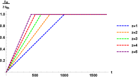
where the first therm is twice the thermodynamic entropy of a black brane. Notice that is independent of time. Therefore, at late times the presence of the island leads to saturate. In figure 2, is plotted for different values of the exponents and of the black brane geometry. At late times, before the Page time, has a linear growth (See eq. (44)). However, after the Page time, it is independent of time (See eq. (84)).

On the other hand, by equating eqs. (44) and (84), the Page time is obtained as follows
| (85) | |||||
| (87) |
Therefore, the Page time is proportional to and depends on both the exponents and of the black brane geometry. It should be pointed out that for and the black brane geometry becomes a d+2 dimensional planar AdS-Schwarzschild black hole. In this case, our results for reduce to those reported in section 5 of ref. Alishahiha:2020qza . 191919Note that in ref. Alishahiha:2020qza , one should turn off all of the higher derivative couplings in the action of the critical gravity to get an AdS-Schwarzschild black hole in Einstein gravity. Moreover, in the left panel of figure 3, is plotted as a function of for different values of . It is observed that is a decreasing function of . Furthermore, in the right panel of figure 3, is plotted as a function of for some values of . It is observed that is an increasing function of . Form these diagrams, it is evident that for , the Page time is always smaller than that for the case and . In other words, the entropy of Hawking radiation for a HV black brane with , saturates sooner than that for a planar AdS-Schwarzschild black hole. However, for positive values of , by decreasing , the Page time can become larger than that for the case and .


4 Entropy of Hawking Radiation: Matter HV QFT
In this section, we study the entropy of Hawking radiation for the case where the matter fields are described by a d+2 dimensional HV QFT which has a dual gravity that is a d+3 dimensional HV geometry at zero temperature. The metric of this geometry is simply obtained by setting in eq. (11) as follows Charmousis:2010zz 202020Note that to have a d+3 dimensional dual gravity we also replace with in eq. (88). 212121Some measures of quantum entanglement such as holographic entanglement entropy, mutual information and entanglement wedge cross section were studied for this background in the literature. See, e. g. Alishahiha:2012cm ; Alishahiha:2015goa ; MohammadiMozaffar:2015wnx ; BabaeiVelni:2019pkw ; Khoeini-Moghaddam:2020ymm ; Dong:2012se ; Tanhayi:2017wcd ; Fischler:2012uv ; Bueno:2014oua ; Cavini:2019wyb , which is not an exhaustive list.
| (88) |
We denote the dynamical and hyperscaling violation exponents of the corresponding HV QFT by and , respectively to draw a distinction between them and the exponents and of the HV black brane. Moreover, for and , the metric (88) becomes an spacetime which is dual to a . Therefore, in this case, all of the results of this section should reduce to those in the previous section. Another important point is that since the HV QFT has a dual gravity, we can apply the RT formula Ryu:2006bv for the calculation of the EE of matter fields as well as the entropy of Hawking radiation.
4.1 Holographic Entanglement Entropy in a d+2 Dimensional HV QFT
Now, we review the holographic entanglement entropy (HEE) for the metric (88) which is derived in ref. Dong:2012se . We consider an entangling region in the shape of a strip on a constant time slice of the dual QFT whose width in the direction is , and denote its lengths along the directions by . It was observed that for , the dual QFT has a Fermi surface and the HEE is given by Dong:2012se
| (89) |
where is Newton’s constant in d+3 dimensions, and is the cutoff in the dual QFT. 222222One might regard the HV QFT as an IR theory which can be obtained by a deformation of a CFT in the UV. In this sense, the cutoff should be considered as an effective cutoff Shaghoulian:2011aa . When the HV QFT has a Fermi surface, one has , where is the radius of the corresponding Fermi surface Shaghoulian:2011aa . In other words, the gravity with the metric in eq. (88) is well defined only above a dynamical scale i.e. Shaghoulian:2011aa ; Dong:2012se (Notice that our radial coordinate is related to that in ref. Dong:2012se by ). In this manner, the cutoff dependent terms in the HEE are IR effects and not divergent in the UV. We would like to thank Edgar Shaghoulian very much for his helpful comments on this topic. On the other hand, for , the HEE is given by Dong:2012se
| (90) |
where
| (91) |
In the following, we renormalize Newton’s constant to absorb the cutoff dependent terms in the HEE. For , from eq. (89), one can renormalize Newton’s constant as follows
| (92) |
However, for , from eq. (90), one has 232323Notice that we set the dynamical scale to one. Otherwise, it is written as .
| (93) |
Notice that for , it reduces to eq. (20). Therefore, we only consider those parts of which are independent of the cutoff in what follows and again rewrite as eq. (21). Moreover, as mentioned in section 3, due to the translational symmetry of the metric (11) along the traverse directions , one might effectively work in two dimensions parametrized by the coordinates and . Therefore, we need to know the HEE of an interval in a two dimensional HV QFT to calculate the entropy of Hawking radiation. 242424Note that to have a two-dimensional HV QFT, one should set in eq. (88). In this case, the cutoff independent parts of the HEE are as follows
-
•
For , by applying eq. (89), one has
(94) where 252525Recall that we set the AdS radius to one.
(95) Notice that, for and , the HV becomes a holographic , and hence ”A” is equal to the corresponding central charge Brown:1986 .
-
•
For , by applying eq. (90), one has
(96)
where
| (97) |
Notice that in this case is negative (positive) when is negative (positive). Moreover, we impose the constraint which for leads to
| (98) |
In the next section, we calculate the entropy of Hawking radiation for the case where the matter QFT is a d+2 dimensional HV QFT. We study the two cases and , separately. Moreover, to have a positive entropy of Hawking radiation when there are no islands and , the finite part of the EE of matter has to be positive, i.e. . Combining this inequality with eq. (98) leads to the constraint .
4.2 Entropy of Hawking Radiation for
In this section, we study the case where the hyperscaling violation exponent of the matter fields is zero. We first assume that there are no islands and calculate the entropy of Hawking radiation. We will see that it grows linearly in time and violates the unitarity, i.e. eq. (2). Therefore, one needs to include the contribution of an island to stop this growth and saturate the entropy of Hawking radiation.
4.2.1 No Islands
In this case, there are only the radiation regions (See the left panel of figure 1). Similar to the previous section, we assume that the whole state on the Cauchy slice is pure. Therefore, one can calculate the EE of the matter fields on the interval instead of that on the region , and hence the entropy of Hawking radiation is simply given by
| (99) |
Next, by applying eqs. (36) and (94), one can rewrite eq. (99) as follows
| (100) |
It grows quadratically in time at early times, i.e. ,
| (101) |
On the other hand, it grows linearly in time at late times, i.e. ,
| (102) |
which again will exceed the coarse-grained entropy of the two black branes. In the next section, we will see that by adding the contribution of an island to the entropy of Hawking radiation, it saturates after the Page time.
4.2.2 With Islands
In this section, we assume that there is an island whose endpoints are located outside the event horizon (See the right panel of figure 1). By assuming that the state on the whole Cauchy slice is pure, one needs to calculate the EE of matter fields on the two disjoint intervals . Since the matter HV QFT has a holographic gravitational theory, one may apply the holographic prescription of ref. Headrick:2010zt to calculate the EE of the two disjoint intervals. In this case, it is given by
| (103) |
where and are the HEE of the connected and disconnected configurations for the corresponding RT surfaces, respectively. Recall that in the connected configuration, each RT surface starts from an endpoint of one of the intervals and ends on an endpoint of another interval (See the left panel of figure 4). However, in the disconnected configuration, each RT surface starts from an endpoint of one interval and ends on another endpoint of the same interval (See the right panel of figure 4). From figure 4, it is evident that for the intervals and , one can find
| (104) | |||||
| (106) |
In the following, we consider two regimes: early times and late times.


At early times, i.e. , the two endpoints of the island are close to each other. In this case, the lengths of the two intervals and are much larger than the distance between them. Therefore, the EE is given by that of the connected RT surfaces (See the left panel of figure 4)
| (107) |
Next, by plugging eq. (36) and (94) into (107), one can find the finite part of the EE of the matter as follows
| (108) | |||||
| (110) |
Therefore the generalized entropy is given by
| (111) | |||||
| (113) |
Now, one can extremize with respect to . If one assumes that and expands in powers of , one obtains
| (114) |
Then, it can be easily solved to find
| (115) |
Next, by plugging eq. (115) into (113) and extremizing with respect to , one simply obtains . It is straightforward to check that for these values of and , the generalized entropy is imaginary. Therefore, one may conclude that at early times there are no islands and the entropy of Hawking radiation is given by eq. (100).
On the other hand, at late times, i.e. , the two endpoints of the island are very far from each other. Therefore, the lengths of the two intervals and are much smaller than their distance. In this case, the EE is given by that of the disconnected RT surfaces (See the right panel of figure 4)
262626It should be pointed out that this prescription were also applied in refs. Almheiri:2019yqk ; Penington:2019kki ; Almheiri:2019qdq ; Hartman:2020swn for two-dimensional eternal black holes at late times.
| (116) |
Next, by plugging eqs. (36) and (94) into (116), one has
At late times, by assuming that and , one can apply the approximation given in eq. (68). After adding the gravitational part, one has
| (120) | |||||
Next, by extremizing the generalized entropy with respect to , one easily finds
| (121) |
Then one can extremize with respect to and expand in powers of as follows
| (124) | |||||
The above equation can be easily solved to find the value of as follows
| (125) |
At the end, by plugging eqs. (121) and (125) into (120), one can obtain the entropy of Hawking radiation as follows
| (128) | |||||
The first term is twice the thermal entropy of the black brane. Moreover, is independent of time. Therefore, the presence of the island at late times leads to become a constant.
Furthermore, by equating eqs. (102) and (128), one can obtain the Page time as follows
| (129) | |||||
| (131) |
Therefore, the Page time is proportional to and depends on both the exponents and of the black brane geometry. Moreover, it is independent of the exponent of the matter fields. It should be pointed out that for and , the HV reduces to a . In this case, becomes equal to the central charge of the CFT. Therefore, it is expected that all of the results in this section reduces to those in section 3, if one sets . On the other hand, we observed that the EE of matter fields, and hence are independent of the dynamical exponent of the matter fields. Therefore, all of the results in this section for , are the same as those for the matter CFT if one replaces with . Therefore, the Page curve and Page time are again given by figures 2 and 3, respectively if one replaces with .
4.3 Entropy of Hawking Radiation for
In this section, we study the case where the hyperscaling violation exponent of matter fields is non-zero. We first study the case where there is no island. Next, we consider the effect of the presence of an island on the entropy of Hawking radiation.
4.3.1 No Islands
When there are no islands, by applying eq. (96), one can write
| (132) |
where is the hyperscaling violating exponent of the matter fields and is defined by eq. (97). Notice that for negative values of , is negative. Therefore, in the following we restrict ourselves to the case . At early times, one has
| (133) |
Thus, grows quadratically in time. On the other hand, at late times, one obtains
| (134) |
Notice that and , and hence the entropy of Hawking radiation grows exponentially in time. This behavior is in contrast to the usual linear growth which were previously observed for flat or AdS black holes in the literature, e.g. refs. Hashimoto:2020cas ; Alishahiha:2020qza .
4.3.2 With Islands
As mentioned before, the EE of the matter fields at early times is given by that of the connected RT surfaces (See the left panel of figure 4). By applying eqs. (36) and (96), one has
| (135) | |||||
| (137) |
After adding the gravitational part, the generalized entropy is given by
| (140) | |||||
| (144) | |||||
Next, by extremizing the above expression with respect to , one obtains . On the other hand, after extermization with respect to one arrives at
| (145) |
which gives the following expression for
| (146) |
It is straightforward to verify that for these values of and , the entropy of Hawking radiation is imaginary. Therefore, one might conclude that there are no islands at early times.
On the other hand, at late times, the EE of matter fields is given by that of the disconnected RT surfaces. In this case, by plugging eq. (96) into eq. (116), one has
| (147) | |||||
At late times, by applying the approximation given in eq. (68), one obtains
| (152) | |||||
Next, by extremizing with respect to , one finds
| (153) |
On the other hand, by plugging eq. (153) into eq. (152) and extremizing with respect to , one has
| (154) |
where and
| (155) | |||||
| (159) | |||||
| (161) |
From eq. (154), one simply obtains
| (162) |
At the end, by plugging eqs. (153) and (162) into eq. (152), the entropy of Hawking radiation is obtained as follows
| (163) |
which is constant in time. Therefore, saturates when there is an island. In figure 5, the entropy of Hawking radiation is plotted as a function of , and . At late times, before the Page time, shows an exponential growth in time (See eq. (134)). However, after the Page time, it saturates (See eq. (163)).


On the other hand, by equating eqs. (134) and (163), the Page time is simply obtained as follows
| (164) |
Therefore , which is a consequence of the exponential growth of with time before reaching the page time (See eq. (134)). In figure 6, the Page time is plotted as a function of and of the black brane. It is observed that is a decreasing function of the exponent . However, it is an increasing function of . On the other hand, in figure 7, the Page time is plotted in terms of which shows that it is a decreasing function of .


5 Discussion
In this paper we studied the Page curve for a two-sided Hyperscaling Violating (HV) black brane in dimensions. We assumed that the matter fields in the black brane geometry and inside the baths are the same. Moreover, we considered two different situations for the matter fields: First, they are described by a . Second, they are described by a d+2 dimensional HV QFT which is dual to a d+3 dimensional gravity that is a HV geometry at zero temperature (See eq. (88)). In both cases, it was observed that at very early times there are no islands. However at late times the presence of an island is necessary to obtain a correct Page curve for the entropy of the Hawking radiation.
For matter CFT, at early times there are no islands. In this case, the entropy of Hawking radiation shows a quadratic growth in time (See eq. (43)). Next, it grows linearly with time (See eq. (44)). If there are no islands, exceeds twice the coarse-grained (thermodynamic) entropy of the black brane. However, when there is an island, becomes a constant (See eq. (84)). The corresponding Page curve is plotted in figure 2 for different values of the exponents and of the black brane.
On the other hand, the Page time is proportional to (See eq. (87)), where and are the thermal entropy and temperature of the black brane, and is the central charge of the matter CFT. Moreover, in figure 3, the Page time is plotted as a function of and . It was observed that is a decreasing function of . On the other hand, it is an increasing function of . Moreover, for , the Page time is always smaller than that for the case and . In other words, the entropy of Hawking radiation for HV black branes saturates sooner than that for planar AdS-Schwarzschild black holes, if one has . However, for positive values of , the Page time becomes larger than that for the case and , if one decreases .
It should be emphasized that for and , the black brane geometry reduces to a dimensional planar AdS-Schwarzschild black hole. Therefore all of our results can be applied for this type of black hole, if one sets and . We verified that for , our results are consistent with those for a four dimensional planar AdS-Schwarzschild black hole in the critical gravity model reported in ref. Alishahiha:2020qza , if one sets all of the higher derivative couplings in the action to zero.
On the other hand, we studied the case where the matter is described by a d+2 dimensional HV QFT. In this case one can assign two exponents and to the matter. Moreover, since the EE of matter is independent of the exponent , the entropy of Hawking radiation is also independent of . In other words, it only depends on the exponent . We examined the two cases and separately. Moreover, since the HV QFT has a dual gravity, we applied the holographic prescription of ref. Headrick:2010zt to calculate the EE of the matter fields on the two disjoint intervals when there is an island (See figure 4). In other words, at early times when the two intervals and are close to each other, we considered the connected RT surfaces. However, at late times when the two intervals are very far from each other, we applied the disconnected RT surfaces. It was observed that:
For , the behaviors of the Page curve and Page time are the same as those for matter CFT. In other words, at early times there are no islands. In this case, shows a quadratic growth in time (See eq. (101)). Next, it grows linearly with time (See eq. (102)). If there are no islands, again exceeds twice the coarse-grained entropy of the black brane. However, when there is an island, becomes a constant (See eq. (163)). Moreover, the Page time is proportional to (See eq. (131)) where .
It should be pointed out that the EE of matter fields, and hence the entropy of Hawking radiation is independent of . On the other hand, for and , the HV becomes a . Therefore, all of the results for should be the same as those for the case where the matter fields are described by a . In particular, the plots of the Page curve and Page time are again given by figures 2 and 3, if one replaces with in the formulas. This observation shows that by applying the holographic prescription of ref. Headrick:2010zt , the entropy of Hawking radiation obeys the expected Page curve. Furthermore, is a decreasing function of the exponent and an increasing function of (See figure 3).
For , it was verified that at early times there are no islands. In the absence of an island, at the beginning again shows a quadratic behavior with time (See eq. (133)). Next, it grows exponentially with time (see eq. (134)), which is in contrast to the usual linear growth for flat and AdS black holes with matter CFT. If there are no islands, again the entropy of Hawking radiation exceeds twice the coarse-grained entropy of the black brane.
However, when there is an island, becomes independent of time (See eq. (163)). This behavior is a consequence of the exponential growth of the entropy of Hawking radiation before the Page time. Moreover, the corresponding Page curve is plotted in figure 5 for different values of the exponent , and . It was also observed that the Page time is proportional to (See eq. (164)). Furthermore, similar to the case , the Page time is a decreasing function of and an increasing function of (See figure 6). Moreover, is independent of and is a decreasing function of (See figure 7).
As mentioned before, for , the EE of radiation grows exponentially before the Page time (see eq. (134)). As long as we know, this rate of growth for the EE is surprising.
272727We would like to thank the referee for her/his enlightening comments on this point.
More precisely, the rate of growth of the EE for Vaidya black branes with Hyperscaling Violation when the entangling region is in the shape of a strip with width and lengths were explored in refs. Alishahiha:2014cwa ; Fonda:2014ula . It was observed that there are three phases for the growth of the EE: First, early times, i.e. where and are the horizon radius and temperature of the black brane, it obeys a power law behavior and is given by
| (165) |
where is the difference of the EE with that of the vacuum and is related to the mass of the black brane. Notice that it is independent of . For and , where the HV QFT becomes a CFT, it is quadratic in time as it is expected for holographic CFTs Liu:2013iza ; Liu:2013qca . Moreover, for very large , it becomes linear in time. Second, at intermediate times, i.e. , it grows linearly in time
| (166) |
where is the entanglement velocity and given by
| (167) |
Third, it saturates to a constant value at late times. Therefore, this exponential growth is a new feature and it would be very interesting to investigate it further and to explore whether or not this growth rate is consistent with unitarity.
At the end, it would also be interesting to do these calculations for one-sided HV black branes and two-sided charged HV black branes and study the effects of the exponents and on the Page curve and Page time.
Acknowledgment
We would like to thank Mohsen Alishahiha very much for his support and illuminating comments during this work. We are also very grateful to Mukund Rangamani, Edgar Shaghoulian, Ali Naseh, Amir Hossein Tajdini, Pablo Bueno and Amin Faraji Astaneh for having very helpful discussions. The work of the author is supported by the school of physics at IPM and Iran Science Elites Federation (ISEF).
References
- (1) S. W. Hawking, “Particle Creation by Black Holes,” Commun. Math. Phys. 43, 199-220 (1975) [erratum: Commun. Math. Phys. 46, 206 (1976)].
- (2) S. W. Hawking, “Breakdown of Predictability in Gravitational Collapse,” Phys. Rev. D 14, 2460-2473 (1976).
- (3) D. N. Page, “Time Dependence of Hawking Radiation Entropy,” JCAP 09, 028 (2013) [arXiv:1301.4995 [hep-th]].
- (4) A. Almheiri, T. Hartman, J. Maldacena, E. Shaghoulian and A. Tajdini, “The entropy of Hawking radiation,” Rev. Mod. Phys. 93, no.3, 035002 (2021) [arXiv:2006.06872 [hep-th]].
- (5) D. N. Page, “Information in black hole radiation,” Phys. Rev. Lett. 71, 3743-3746 (1993) [arXiv:hep-th/9306083 [hep-th]].
- (6) G. Penington, “Entanglement Wedge Reconstruction and the Information Paradox,” JHEP 09, 002 (2020) [arXiv:1905.08255 [hep-th]].
- (7) A. Almheiri, N. Engelhardt, D. Marolf and H. Maxfield, “The entropy of bulk quantum fields and the entanglement wedge of an evaporating black hole,” JHEP 12, 063 (2019) [arXiv:1905.08762 [hep-th]].
- (8) A. Almheiri, R. Mahajan, J. Maldacena and Y. Zhao, “The Page curve of Hawking radiation from semiclassical geometry,” JHEP 03, 149 (2020) [arXiv:1908.10996 [hep-th]].
- (9) A. Almheiri, R. Mahajan and J. Maldacena, “Islands outside the horizon,” [arXiv:1910.11077 [hep-th]].
- (10) J. M. Maldacena, “The Large N limit of superconformal field theories and supergravity,” Int. J. Theor. Phys. 38, 1113-1133 (1999) [arXiv:hep-th/9711200 [hep-th]].
- (11) N. Engelhardt and A. C. Wall, “Quantum Extremal Surfaces: Holographic Entanglement Entropy beyond the Classical Regime,” JHEP 01, 073 (2015) [arXiv:1408.3203 [hep-th]].
- (12) S. Ryu and T. Takayanagi, “Holographic derivation of entanglement entropy from AdS/CFT,” Phys. Rev. Lett. 96, 181602 (2006) [arXiv:hep-th/0603001 [hep-th]].
- (13) V. E. Hubeny, M. Rangamani and T. Takayanagi, “A Covariant holographic entanglement entropy proposal,” JHEP 07, 062 (2007) [arXiv:0705.0016 [hep-th]].
- (14) T. Faulkner, A. Lewkowycz and J. Maldacena, “Quantum corrections to holographic entanglement entropy,” JHEP 11, 074 (2013) [arXiv:1307.2892 [hep-th]].
- (15) R. Jackiw, “Lower Dimensional Gravity,” Nucl. Phys. B 252, 343-356 (1985).
- (16) C. Teitelboim, “Gravitation and Hamiltonian Structure in Two Space-Time Dimensions,” Phys. Lett. B 126, 41-45 (1983).
- (17) G. Penington, S. H. Shenker, D. Stanford and Z. Yang, “Replica wormholes and the black hole interior,” [arXiv:1911.11977 [hep-th]].
- (18) A. Almheiri, T. Hartman, J. Maldacena, E. Shaghoulian and A. Tajdini, “Replica Wormholes and the Entropy of Hawking Radiation,” JHEP 05, 013 (2020) [arXiv:1911.12333 [hep-th]].
- (19) K. Goto, T. Hartman and A. Tajdini, “Replica wormholes for an evaporating 2D black hole,” JHEP 04, 289 (2021) [arXiv:2011.09043 [hep-th]].
- (20) D. Marolf and H. Maxfield, “Observations of Hawking radiation: the Page curve and baby universes,” JHEP 04, 272 (2021) [arXiv:2010.06602 [hep-th]].
- (21) R. Bousso and A. Shahbazi-Moghaddam, “Island Finder and Entropy Bound,” Phys. Rev. D 103, no.10, 106005 (2021) [arXiv:2101.11648 [hep-th]].
- (22) J. F. Pedraza, A. Svesko, W. Sybesma and M. R. Visser, “Microcanonical Action and the Entropy of Hawking Radiation,” [arXiv:2111.06912 [hep-th]].
- (23) A. Lewkowycz and J. Maldacena, “Generalized gravitational entropy,” JHEP 08, 090 (2013) [arXiv:1304.4926 [hep-th]].
- (24) X. Dong, A. Lewkowycz and M. Rangamani, “Deriving covariant holographic entanglement,” JHEP 11, 028 (2016) [arXiv:1607.07506 [hep-th]].
- (25) H. Z. Chen, Z. Fisher, J. Hernandez, R. C. Myers and S. M. Ruan, “Information Flow in Black Hole Evaporation,” JHEP 03, 152 (2020) [arXiv:1911.03402 [hep-th]].
- (26) T. J. Hollowood and S. P. Kumar, “Islands and Page Curves for Evaporating Black Holes in JT Gravity,” JHEP 08, 094 (2020) [arXiv:2004.14944 [hep-th]].
- (27) H. Z. Chen, Z. Fisher, J. Hernandez, R. C. Myers and S. M. Ruan, “Evaporating Black Holes Coupled to a Thermal Bath,” JHEP 01, 065 (2021) [arXiv:2007.11658 [hep-th]].
- (28) V. Balasubramanian, B. Craps, M. Khramtsov and E. Shaghoulian, “Submerging islands through thermalization,” JHEP 10, 048 (2021) [arXiv:2107.14746 [hep-th]].
- (29) F. F. Gautason, L. Schneiderbauer, W. Sybesma and L. Thorlacius, “Page Curve for an Evaporating Black Hole,” JHEP 05, 091 (2020) [arXiv:2004.00598 [hep-th]].
- (30) T. Anegawa and N. Iizuka, “Notes on islands in asymptotically flat 2d dilaton black holes,” JHEP 07, 036 (2020) [arXiv:2004.01601 [hep-th]].
- (31) X. Wang, R. Li and J. Wang, “Page curves for a family of exactly solvable evaporating black holes,” Phys. Rev. D 103, no.12, 126026 (2021) [arXiv:2104.00224 [hep-th]].
- (32) T. Hartman, E. Shaghoulian and A. Strominger, “Islands in Asymptotically Flat 2D Gravity,” JHEP 07, 022 (2020) [arXiv:2004.13857 [hep-th]].
- (33) S. He, Y. Sun, L. Zhao and Y. X. Zhang, “The universality of islands outside the horizon,” [arXiv:2110.07598 [hep-th]].
- (34) A. Almheiri, R. Mahajan and J. E. Santos, “Entanglement islands in higher dimensions,” SciPost Phys. 9, no.1, 001 (2020) [arXiv:1911.09666 [hep-th]].
- (35) K. Hashimoto, N. Iizuka and Y. Matsuo, “Islands in Schwarzschild black holes,” JHEP 06, 085 (2020) [arXiv:2004.05863 [hep-th]].
- (36) H. Geng and A. Karch, “Massive islands,” JHEP 09, 121 (2020) [arXiv:2006.02438 [hep-th]].
- (37) H. Z. Chen, R. C. Myers, D. Neuenfeld, I. A. Reyes and J. Sandor, “Quantum Extremal Islands Made Easy, Part I: Entanglement on the Brane,” JHEP 10, 166 (2020) [arXiv:2006.04851 [hep-th]].
- (38) K. Ghosh and C. Krishnan, “Dirichlet baths and the not-so-fine-grained Page curve,” JHEP 08, 119 (2021) [arXiv:2103.17253 [hep-th]].
- (39) C. Krishnan, “Critical Islands,” JHEP 01, 179 (2021) [arXiv:2007.06551 [hep-th]].
- (40) H. Z. Chen, R. C. Myers, D. Neuenfeld, I. A. Reyes and J. Sandor, “Quantum Extremal Islands Made Easy, Part II: Black Holes on the Brane,” JHEP 12, 025 (2020) [arXiv:2010.00018 [hep-th]].
- (41) Y. Matsuo, “Islands and stretched horizon,” JHEP 07, 051 (2021) [arXiv:2011.08814 [hep-th]].
- (42) G. K. Karananas, A. Kehagias and J. Taskas, “Islands in linear dilaton black holes,” JHEP 03, 253 (2021) [arXiv:2101.00024 [hep-th]].
- (43) A. Saha, S. Gangopadhyay and J. P. Saha, “Mutual information, islands in black holes and the Page curve,” [arXiv:2109.02996 [hep-th]].
- (44) I. Aref’eva and I. Volovich, “A Note on Islands in Schwarzschild Black Holes,” [arXiv:2110.04233 [hep-th]].
- (45) M. Alishahiha, A. Faraji Astaneh and A. Naseh, “Island in the presence of higher derivative terms,” JHEP 02, 035 (2021) [arXiv:2005.08715 [hep-th]].
- (46) Y. Ling, Y. Liu and Z. Y. Xian, “Island in Charged Black Holes,” JHEP 03, 251 (2021) [arXiv:2010.00037 [hep-th]].
- (47) X. Wang, R. Li and J. Wang, “Islands and Page curves of Reissner-Nordström black holes,” JHEP 04, 103 (2021) [arXiv:2101.06867 [hep-th]].
- (48) W. Kim and M. Nam, “Entanglement entropy of asymptotically flat non-extremal and extremal black holes with an island,” Eur. Phys. J. C 81, no.10, 869 (2021) [arXiv:2103.16163 [hep-th]].
- (49) M. H. Yu and X. H. Ge, “Page Curves and Islands in Charged Dilaton Black Holes,” [arXiv:2107.03031 [hep-th]].
- (50) B. Ahn, S. E. Bak, H. S. Jeong, K. Y. Kim and Y. W. Sun, “Islands in charged linear dilaton black holes,” [arXiv:2107.07444 [hep-th]].
- (51) V. Balasubramanian, A. Kar, O. Parrikar, G. Sárosi and T. Ugajin, “Geometric secret sharing in a model of Hawking radiation,” JHEP 01, 177 (2021) [arXiv:2003.05448 [hep-th]].
- (52) S. Fallows and S. F. Ross, “Islands and mixed states in closed universes,” JHEP 07, 022 (2021) [arXiv:2103.14364 [hep-th]].
- (53) L. Anderson, O. Parrikar and R. M. Soni, “Islands with gravitating baths: towards ER = EPR,” JHEP 21, 226 (2020) [arXiv:2103.14746 [hep-th]].
- (54) H. Geng, A. Karch, C. Perez-Pardavila, S. Raju, L. Randall, M. Riojas and S. Shashi, “Information Transfer with a Gravitating Bath,” SciPost Phys. 10, no.5, 103 (2021) [arXiv:2012.04671 [hep-th]].
- (55) H. Geng, S. Lüst, R. K. Mishra and D. Wakeham, “Holographic BCFTs and Communicating Black Holes,” jhep 08, 003 (2021) [arXiv:2104.07039 [hep-th]].
- (56) V. Balasubramanian, A. Kar and T. Ugajin, “Entanglement between two gravitating universes,” [arXiv:2104.13383 [hep-th]].
- (57) A. Almheiri, A. Mousatov and M. Shyani, “Escaping the Interiors of Pure Boundary-State Black Holes,” [arXiv:1803.04434 [hep-th]].
- (58) I. Kourkoulou and J. Maldacena, “Pure states in the SYK model and nearly- gravity,” [arXiv:1707.02325 [hep-th]].
- (59) S. Cooper, M. Rozali, B. Swingle, M. Van Raamsdonk, C. Waddell and D. Wakeham, “Black hole microstate cosmology,” JHEP 07, 065 (2019) [arXiv:1810.10601 [hep-th]].
- (60) F. Omidi, “Regularizations of Action-Complexity for a Pure BTZ Black Hole Microstate,” JHEP 07, 020 (2020) [arXiv:2004.11628 [hep-th]].
- (61) T. Hartman, Y. Jiang and E. Shaghoulian, “Islands in cosmology,” JHEP 11, 111 (2020) [arXiv:2008.01022 [hep-th]].
- (62) V. Balasubramanian, A. Kar and T. Ugajin, “Islands in de Sitter space,” JHEP 02, 072 (2021) [arXiv:2008.05275 [hep-th]].
- (63) W. Sybesma, “Pure de Sitter space and the island moving back in time,” Class. Quant. Grav. 38, no.14, 145012 (2021) [arXiv:2008.07994 [hep-th]].
- (64) H. Geng, Y. Nomura and H. Y. Sun, “Information paradox and its resolution in de Sitter holography,” Phys. Rev. D 103, no.12, 126004 (2021) [arXiv:2103.07477 [hep-th]].
- (65) L. Aalsma and W. Sybesma, “The Price of Curiosity: Information Recovery in de Sitter Space,” JHEP 05, 291 (2021) [arXiv:2104.00006 [hep-th]].
- (66) Y. Chen, V. Gorbenko and J. Maldacena, “Bra-ket wormholes in gravitationally prepared states,” JHEP 02, 009 (2021) [arXiv:2007.16091 [hep-th]].
- (67) S. Azarnia, R. Fareghbal, A. Naseh and H. Zolfi, “Islands in Flat-Space Cosmology,” [arXiv:2109.04795 [hep-th]].
- (68) V. Balasubramanian, A. Kar and T. Ugajin, “Entanglement between two disjoint universes,” JHEP 02, 136 (2021) [arXiv:2008.05274 [hep-th]].
- (69) A. Miyata and T. Ugajin, “Evaporation of black holes in flat space entangled with an auxiliary universe,” [arXiv:2104.00183 [hep-th]].
- (70) A. Miyata and T. Ugajin, “Entanglement between two evaporating black holes,” [arXiv:2111.11688 [hep-th]].
- (71) M. Alishahiha, E. O Colgain and H. Yavartanoo, “Charged Black Branes with Hyperscaling Violating Factor,” JHEP 11, 137 (2012) [arXiv:1209.3946 [hep-th]].
- (72) L. Susskind and J. Uglum, “Black hole entropy in canonical quantum gravity and superstring theory,” Phys. Rev. D 50, 2700-2711 (1994) [arXiv:hep-th/9401070 [hep-th]].
- (73) R. Bousso, Z. Fisher, S. Leichenauer and A. C. Wall, “Quantum focusing conjecture,” Phys. Rev. D 93, no.6, 064044 (2016) [arXiv:1506.02669 [hep-th]].
- (74) L. Bombelli, R. K. Koul, J. Lee and R. D. Sorkin, “A Quantum Source of Entropy for Black Holes,” Phys. Rev. D 34, 373-383 (1986).
- (75) M. Srednicki, Phys. Rev. Lett. 71, 666-669 (1993) doi:10.1103/PhysRevLett.71.666 [arXiv:hep-th/9303048 [hep-th]].
- (76) S. Ryu and T. Takayanagi, “Aspects of Holographic Entanglement Entropy,” JHEP 08, 045 (2006) [arXiv:hep-th/0605073 [hep-th]].
- (77) C. Holzhey, F. Larsen and F. Wilczek, “Geometric and renormalized entropy in conformal field theory,” Nucl. Phys. B 424, 443-467 (1994) [arXiv:hep-th/9403108 [hep-th]].
- (78) P. Calabrese and J. L. Cardy, “Entanglement entropy and quantum field theory,” J. Stat. Mech. 0406, P06002 (2004) [arXiv:hep-th/0405152 [hep-th]].
- (79) P. Calabrese, J. Cardy and E. Tonni, “Entanglement entropy of two disjoint intervals in conformal field theory,” J. Stat. Mech. 0911, P11001 (2009) [arXiv:0905.2069 [hep-th]].
- (80) P. Calabrese and J. Cardy, “Entanglement entropy and conformal field theory,” J. Phys. A 42, 504005 (2009) [arXiv:0905.4013 [cond-mat.stat-mech]].
- (81) H. Casini, C. D. Fosco and M. Huerta, “Entanglement and alpha entropies for a massive Dirac field in two dimensions,” J. Stat. Mech. 0507, P07007 (2005) [arXiv:cond-mat/0505563 [cond-mat]].
- (82) H. Casini and M. Huerta, “Remarks on the entanglement entropy for disconnected regions,” JHEP 03, 048 (2009) [arXiv:0812.1773 [hep-th]].
- (83) H. Casini and M. Huerta, “Reduced density matrix and internal dynamics for multicomponent regions,” Class. Quant. Grav. 26, 185005 (2009) [arXiv:0903.5284 [hep-th]].
- (84) C. Charmousis, B. Gouteraux, B. S. Kim, E. Kiritsis and R. Meyer, “Effective Holographic Theories for low-temperature condensed matter systems,” JHEP 11, 151 (2010) [arXiv:1005.4690 [hep-th]].
- (85) X. Dong, S. Harrison, S. Kachru, G. Torroba and H. Wang, “Aspects of holography for theories with hyperscaling violation,” JHEP 06, 041 (2012) [arXiv:1201.1905 [hep-th]].
- (86) E. Shaghoulian, “Holographic Entanglement Entropy and Fermi Surfaces,” JHEP 05, 065 (2012) [arXiv:1112.2702 [hep-th]].
- (87) Brown, J.D., Henneaux, M. Central charges in the canonical realization of asymptotic symmetries: An example from three dimensional gravity. Commun.Math. Phys. 104, 207–226 (1986).
- (88) M. Alishahiha and H. Yavartanoo, “On Holography with Hyperscaling Violation,” JHEP 11, 034 (2012) [arXiv:1208.6197 [hep-th]].
- (89) W. Fischler, A. Kundu and S. Kundu, “Holographic Mutual Information at Finite Temperature,” Phys. Rev. D 87, no.12, 126012 (2013) [arXiv:1212.4764 [hep-th]].
- (90) P. Bueno and P. F. Ramirez, “Higher-curvature corrections to holographic entanglement entropy in geometries with hyperscaling violation,” JHEP 12, 078 (2014) [arXiv:1408.6380 [hep-th]].
- (91) M. Alishahiha, A. F. Astaneh, P. Fonda and F. Omidi, “Entanglement Entropy for Singular Surfaces in Hyperscaling violating Theories,” JHEP 09, 172 (2015) [arXiv:1507.05897 [hep-th]].
- (92) M. R. Mohammadi Mozaffar, A. Mollabashi and F. Omidi, “Holographic Mutual Information for Singular Surfaces,” JHEP 12, 082 (2015) [arXiv:1511.00244 [hep-th]].
- (93) M. R. Tanhayi, “Universal terms of holographic entanglement entropy in theories with hyperscaling violation,” Phys. Rev. D 97, no.10, 106008 (2018) [arXiv:1711.10526 [hep-th]].
- (94) K. Babaei Velni, M. R. Mohammadi Mozaffar and M. H. Vahidinia, “Some Aspects of Entanglement Wedge Cross-Section,” JHEP 05, 200 (2019) [arXiv:1903.08490 [hep-th]].
- (95) G. Cavini, D. Seminara, J. Sisti and E. Tonni, “On shape dependence of holographic entanglement entropy in AdS4/CFT3 with Lifshitz scaling and hyperscaling violation,” JHEP 02, 172 (2020) [arXiv:1907.10030 [hep-th]].
- (96) S. Khoeini-Moghaddam, F. Omidi and C. Paul, “Aspects of Hyperscaling Violating Geometries at Finite Cutoff,” JHEP 02, 121 (2021) [arXiv:2011.00305 [hep-th]].
- (97) M. Headrick, “Entanglement Renyi entropies in holographic theories,” Phys. Rev. D 82, 126010 (2010) [arXiv:1006.0047 [hep-th]].
- (98) M. Alishahiha, A. Faraji Astaneh and M. R. Mohammadi Mozaffar, “Thermalization in backgrounds with hyperscaling violating factor,” Phys. Rev. D 90, no.4, 046004 (2014) [arXiv:1401.2807 [hep-th]].
- (99) P. Fonda, L. Franti, V. Keränen, E. Keski-Vakkuri, L. Thorlacius and E. Tonni, “Holographic thermalization with Lifshitz scaling and hyperscaling violation,” JHEP 08, 051 (2014) [arXiv:1401.6088 [hep-th]].
- (100) H. Liu and S. J. Suh, “Entanglement Tsunami: Universal Scaling in Holographic Thermalization,” Phys. Rev. Lett. 112, 011601 (2014) [arXiv:1305.7244 [hep-th]].
- (101) H. Liu and S. J. Suh, “Entanglement growth during thermalization in holographic systems,” Phys. Rev. D 89, no.6, 066012 (2014) [arXiv:1311.1200 [hep-th]].