Entanglement witness for combined atom interferometer-mechanical oscillator setup
Abstract
We investigate how to entangle an atom interferometer and a macroscopic mechanical oscillator in order to create non-classical states of the oscillator. We propose an entanglement witness, from whose violation, the generation of entanglement can be determined. We do this for both the noiseless case and when including thermal noise. Thermal noise can arise from two sources: the first being when the oscillator starts in a thermal state, and the second when a continuous thermal bath is in contact with the oscillator. We find that for the appropriate oscillator quality factor , violation always exists for any value of magnetic coupling and thermal occupancy . Cooling the oscillator to its ground state provides an improvement in the EW violation than starting in a thermal state. However, this still requires at least 105 measurements to be determined. We then consider how to use magnetic interactions to realize this idea.
Entanglement is a core feature of quantum mechanics that precludes any hidden variable classical theory. Many groups have considered entanglement in macroscopic systems, particularly in the case of spin-spin systems [1, 2, 3, 4, 5], oscillator-oscillator systems [6, 7, 8, 9, 10, 11, 12], and spin-oscillator systems [13, 14, 15]. For instance, Kong et al. experimentally generate entanglement between the spins of atoms in a vapor [1], Ockeloen-Korppi et al. use a cavity to entangle two mirrors located 600 µm apart [6], and Riedinger et al. entangle two chips separated by 20 cm [7]. Thomas et al. entangle a spin ensemble with a square membrane of sides 1 mm in length [13].
Of particular interest are approaches to entangle masses and/or spins to investigate theories that incorporate quantum mechanics with gravity. For example, Kafri et al. [16], Bose et al. [2] and Marletto et al. [17] propose using two masses which interact with each other though a gravitational force; if the two masses become entangled, then we can conclude that the gravitational field is capable of generating entanglement. A different approach by Carney et al. [18] suggests gravitationally coupling an atom interferometer with a mechanical oscillator. If the interaction is capable of entanglement, the oscillator and the atoms will get entangled, which can be detected using the interferometer’s signal.
Such experiments have to use certain techniques to determine the existence of entanglement. The experiments in Ref. [1, 6, 7, 13, 2] use (or propose using) an entanglement witness (EW) that work for very low noise situations, where one prepares pure states of the two systems, and noise and decoherence are neglected. An EW is a quantity composed of observables; it has a bound satisfied by separable states, which, if violated, determines that entanglement exists between the systems. The literature on creating an entanglement witness is varied. The most well-known example of EWs might be Bell inequalities [19, 20] used to distinguish between the possibility of local hidden variable theories and entanglement. Another common EW is one which is often applied to oscillator-oscillator entanglement, whose general version was proposed by Duan et al. [21].
In this paper, we work within the context of the proposal by Carney et al. [18], introduced previously. In the progress towards such a gravity experiment, it is more reasonable to first attempt the generation of magnetic entanglement between the atom interferometer and the oscillator, since a sufficiently strong magnetic coupling is easier to obtain. Before proceeding with physically building the experiment, it is important to ensure that entanglement will exist, at least theoretically, and understand the physical parameters at which it will occur. In order to do this, we construct an entanglement witness (EW) for our setup that provides a path for violation at finite motional temperatures and with noise and dephasing. We investigate the effects of thermal noise on its violation and establish the conditions on parameters such that violation exists. We find that for appropriate values of oscillator quality factor , violation always exists for any value of magnetic coupling and thermal occupancy .
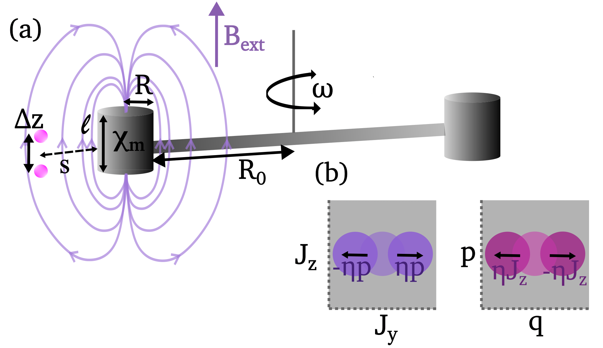
General entanglement witness - A simplified setup that we can consider is shown in Figure 1. The Hamiltonian of the system is (note that herein) [18]
| (1) |
and are the oscillator creation and annihilation operators. is a pseudo-spin operator describing the location of atoms; that is, , where characterizes which of the two interferometer traps the atom is in. As stated earlier, the creation of entanglement between the interferometer and the oscillator can be determined by measuring an entanglement witness (EW). We find that the following quantity is an applicable EW for our setup:
| (2) |
Here, and . The coefficients and can be chosen as appropriate. Such spin-oscillator variances allow for the characterization of spin-oscillator correlations. Eq. 2 is bounded by for all separable states. If this bound is violated by the experimental state of concern, we can conclude that it is an entangled state.
can be derived using the theorem in the paper by Hofmann et al. [23]. They showed that for operators of system and of system , if and , then for any separable state. Starting with , where the summation is over the and components, we follow Ref. [23] to arrive at the general bound . To obtain the witness in Eq. 2, we set and on the left and right hand sides of this inequality.
The oscillator-operator bound can be derived using the Heisenberg uncertainty principle and carrying out a minimization process; we get . In analogy to a derivation in Ref. [23], the general bound for the spin operators is , which for a fully symmetric state will be . The most general case will be where is the minimum value that can take at the time of measurement.
For the EW in Eq. 2, we can finally write the general bound to be
| (3) |
That is, for a separable state, the condition that will be satisfied. If we evaluate with respect to a possibly entangled state in order to obtain the value and find that , then the bound is violated and we can conclude that the state is indeed entangled.
We explore this EW in the context of two scenarios; when the systems are noiseless and when there is thermal noise (the case of atomic dephasing can be found in the Supplementary Material). For each scenario, we determine whether the EW is violated. In an experimental setting, is a theoretical value that we have at hand, while is the quantity that we estimate through measurement. We consider the quantity ; the EW is violated if . Since the imprecision is set by , informs us of the number of measurements required to determine the existence of entanglement, since .
A key step in this process is determining the coefficients and , where we attempt to minimize the variance of the EW. When , finding and that maximizes suffices. Practically, however, finding is complicated due to the absolute value term given by . Therefore, in this paper we minimize the value .
Noiseless entanglement witness - First, we investigate the violation for the noiseless scenario. Here the atomic states starts in the eigenstate and the oscillator in the ground state [18]; after evolving under Eq. 1, the final entangled state is given by (explicit form is given in the Supplemental Material).
We can understand the evolution of the system described by Eq. 1 within the Heisenberg picture. The first component to consider is the Heisenberg operator . The second component is the rotation of the spin operators and about the z-axis by angle , due to the term in the Hamiltonian; this is visually shown in Figure 1. These two components show us that the different operators become correlated with each other, for instance, with . Optimizing the values of and translates to controlling the contributions of these correlations such that the variances of Eq. 2 are minimized for the entangled state. For instance, if we consider the operator combination , to first order in (where ) for simplicity, we have
| (4) |
The first line of Eq. 4 is the Heisenberg-evolved operator expanded to (with the squeezing term dropped). The term added to contributes the coefficients and ; given the explicit form of as shown in the second line of Eq. 4, it seems plausible that values for and can be chosen such that the contribution to from can be canceled. Note that, since we are starting in the state , the operators here evaluate to and the terms evaluate to 0.
If we proceed with solving for and , we see that this does indeed occur. We first expand various products of the operators (, etc.) to ; should be appropriate, since the only other parameter that can greatly “cancel out” the effects of is the number of atoms and the highest order of is (which arises from the squaring of the spin operators). Once we have these Heisenberg-evolved operators and their products, we can evaluate their expectation values with respect to (which is the remainder of ) to obtain .
Now we can minimize with respect to and . We find that
| (5) | ||||
| (6) | ||||
| (7) | ||||
| (8) |
As can be seen, these coefficients and, thereby, the EW of Eq. 2, depend on the following experimental parameters: the coupling , the number of atoms , the mass of the oscillator , oscillator frequency , and the interaction time . Furthermore, these coefficients satisfy .
We can substitute these coefficients into Eq. 4 to see how they can be used to cancel out correlations between operators. If we were to set , we find that .
We can now finally obtain the bound
| (9) |
and the entangled-state value
| (10) |
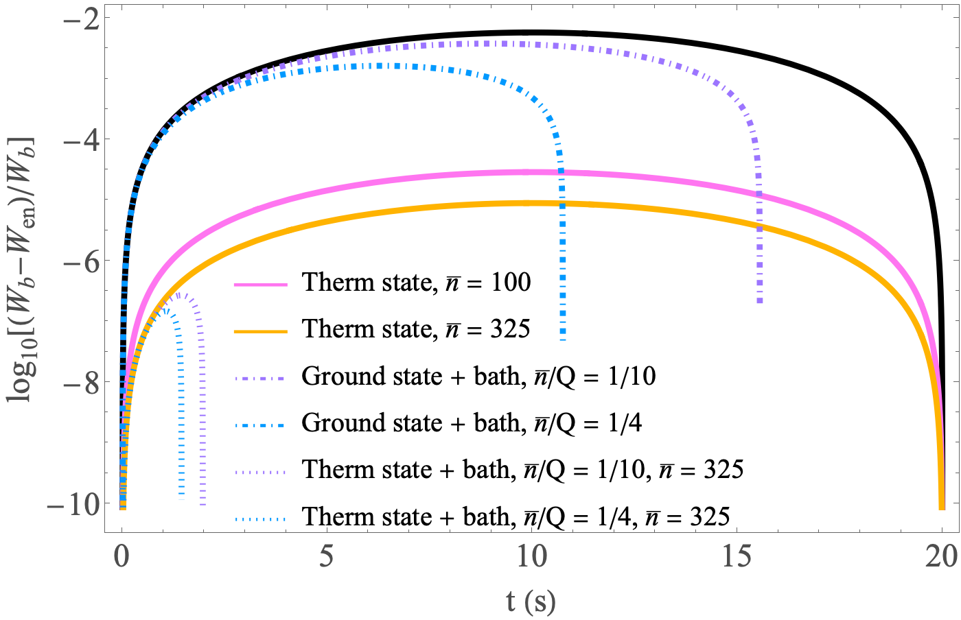
We see that violates the EW bound by a value of . It must be emphasized again that these calculations hold for . The exact limit on is such that Eq. 10 is always positive; that is, the result is valid for , which for would be . Fig. 2 shows a plot of the violation (black line); it is highest at , which is consistent with the results in Carney et al. [18] where the oscillator is completely entangled with the atoms at .
Entanglement witness with a thermal state and white noise bath - We can now consider the case of thermal noise. There are three scenarios that can be considered; the first when the oscillator starts in a thermal state, the second when the oscillator starts in a thermal state and remains in contact with a white noise bath, and the third when the oscillator starts in the ground state and remains in contact with a bath.
For a thermal state [24], we find that, to , the new coefficients are
| (11) | ||||
| (12) | ||||
| (13) | ||||
| (14) |
The next order of these coefficients is . Comparing with Equations 5-8, it can be seen that and have been modified by a factor of . However, they no longer satisfy . As explained previously, and as can be seen by their similar forms, these coefficients work together with the covariances and correlations to minimize the value of when starting in a thermal state.
The bound to is
| (15) |
and the entangled state value of the EW to is
| (16) |
The expansion to is only valid if ; larger leads to key corrections associated with atomic phase evolution of order unity. Plots for different values of are shown in Fig. 2; the higher the value of , the weaker the violation.
Next, we consider a scenario where the oscillator is in continuous contact with white noise, which approximates a thermal bath at high temperature. The Hamiltonian is now given by
| (17) |
where is a classical white noise force; this Hamiltonian is simply that of Eq. 1 to which the effect from has been added. The auto-correlation function is a delta function with an amplitude set by the fluctuation-dissipation theorem . Proceeding to understand within the Heisenberg picture as previously, we can solve for to obtain . With and , the noise contributions to and can be expressed as and . Further, and will rotate about the z-axis by an angle as follows: and . The white noise contribution to this angle is given by . Note that here, and .
Note that , , and are not operators since they arise from the classical noise ; therefore, their covariances consist of averages over classical noise and are hence represented with the notation . For instance, contributes to the noise in the EW term and contributes to the noise in . Therefore, the expectation values that compose the EW must be modified by adding the noise contributions , , , , and ; an appropriate linear combination of these gives . Thus, we now have, , where
| (18) |
with the coefficients being those in Equations 11-14. Note that the terms where appears have been truncated to . The term is unaffected by noise as it commutes through the Hamiltonian. Therefore, for the spin variances, only the term comes into play; starting in eigenstate means that, to , there is no noise contribution from either.
Using the previous bound in Eq. 15, we plot the EW violation in Figure 2 (dotted lines). For violation to take place, the condition that
| (19) |
is required when . The bound is approximately for .
We can further consider the scenario where the oscillator is cooled to its ground state at the start, but remains in contact with a bath for the rest of time; this is given by , with the coefficients of Eqs. 5-8 being used in Eq. 18 (see Supplemental Material for “re-optimized” coefficients). The dot-dashed lines in Fig. 2 shows the violation for different values of . The condition for violation to take place is now
| (20) |
which for is . This is better than for an initial thermal state.
We now investigate the value of the magnetic coupling in Figure 1. A large diamagnetic coupling can be attained by using superconducting masses and placing the atoms in different magnetically sensitive states. For instance, we can place one atom in the state and the other in . In such a scenario, the coupling would primarily be due to the first order Zeeman shift, which is linear in [25]. For a cylinder with mm, , density g/cm3 [26], m, mm, cm, 50 mT, , and , we get . A coupling approximately weaker is available for atomic clock () states. For details on this calculation, see the Supplemental Material; this includes the cylindrical field expressions [27], and calculations for regular metals like tungsten [28, 29].
Conclusion - Within the context of a combined atom interferometer and oscillator system, we can use an entanglement witness to show that entanglement exists even in the case where the oscillator starts in a thermal state and remains in contact with a bath. In fact, we find that for the appropriate oscillator quality factor and thermal occupancy , violation always exists for any value of magnetic coupling . Additionally, an improvement in the EW violation if the oscillator is cooled to its ground state before running the experiment. However, to observe this violation, the number of measurements required would be at least on the order of 105. Hence, experimentally using the proposed EW to measure entanglement may not be ideal; rather our results tell us that with the right physical parameters we can indeed experimentally generate entanglement between an atom interferometer and a mechanical oscillator, even with thermal noise. For practical detection of entanglement, other methods will have to be employed.
Acknowledgments - We would like to acknowledge Yuxin Wang and Jon Kunjummen for conceptual and mathematical discussions. We would also like to thank our collaborators for helping with experimental details and overall discussions, in particular, Jon Pratt, Garrett Louie, Cristian Panda, Prabudhya Bhattacharyya, Matt Tao, Lorenz Keck, James Egelhoff, John Manley, Stephan Schlamminger, Holger Müller, and Daniel Carney. We thank Daniel Barker and John Manley for comments on our paper. The work of G. P. and D. B. was made possible by the Heising-Simons Foundation grant 2023-4467 “Testing the Quantum Coherence of Gravity” and through the support of Grant 63121 from the John Templeton Foundation. The opinions expressed in this publication are those of the authors and do not necessarily reflect the views of the John Templeton Foundation. J. T. is solely funded by the National Institute of Standards and Technology.
I Supplemental Material: Entanglement witness for combined atom interferometer-mechanical oscillator setup
I.1 Entanglement witness
This section provides more details and discussion on the derivation of the entanglement witness and its violation in the noiseless and thermal noise scenarios. Additionally, we add a section on the effects of atomic dephasing.
I.1.1 General entanglement witness form and bound
We investigate the entanglement witness,
| (21) |
As we stated in the main paper, the bound for can be derived using the theorem in the paper by Hofmann et al. [23]: for operators of system and of system , if and , then for any separable state. There is, however, a prerequisite that for each operator there must be a . In the case of Eq. 21, and . It can be seen in Eq. 21 that there is a term with no oscillator operators, and composed of only the spin operator ; we do not measure correlations between and the oscillator operators because the mean of these correlations are zero, at least for the noiseless entangled state in Equation 34. In order to satisfy the requirement of every operator having its counterpart , we started with the term and set the coefficients and to zero after the derivation of the bound. We lay out this derivation here.
Starting with , where the summation is over the and components, we follow Ref. [23] to arrive at the general bound
| (22) |
To obtain the witness in Eq. 21, we set and on the left and right hand sides of the inequality. The oscillator-operator bound can be derived as follows: we have
| (23) |
for which we can apply the Heisenberg uncertain principle
| (24) |
and minimize the R.H.S to give
| (25) |
Setting and , we then find that the sum of the oscillator-operator variances is bounded by
| (26) |
In analogy to a derivation in Ref. [23], the general bound for the spin operators can be obtained as follows:
| (27) |
With and we have
| (28) |
The question now arises as to the exact value of . For a fully symmetric state, we have
| (29) |
Here takes the maximum possible value. Eq. 29 can also be derived from the fact that (shown in Ref. [23]),
| (30) |
Using , the minimum value that will take at the time of measurement, we write the most general bound to be
| (31) |
as in the main paper.
As mentioned, we consider the quantity
| (32) |
when , finding suffices. Practically, however, finding is complicated due to the absolute value term given by . Therefore, in this paper we minimize the value ; that is, we solve for and such that and . , being quadratic in and , is solvable. Note that this gives a higher violation than if were to maximize by expressing the absolute value as , where sets the sign (+1, or -1), for reasons we cannot explain currently; the underlying reason must be that optimizing (and choosing the pairing of and the coefficients which makes this value positive) is not equivalent to optimizing .
and contribute to obtaining by reducing the value of the variance terms in Equation 21. In the most general case, an expansion of Eq. 21 gives
| (33) |
To obtain , the expectation value indicated by is taken by evaluating the operators between the appropriate entangled state denoted by . Observing the terms of , we can see that and characterize the contribution of covariances to the value of the witness; for instance, there are terms such as and . Additionally, as described in the upcoming sections, the spin and oscillator operators get correlated with each other, which can be seen when investigating their evolution in the Heisenberg picture. Therefore, in optimizing for the values of and , we are primarily controlling the contribution of these covariances and correlations, such that we obtain .
I.1.2 Noiseless entanglement witness
The noiseless entangled state of our system is given by [18]
| (34) |
Compared with Ref. [18], we have dropped the squeezing term, because it’s likely to be of given the size of the coupling .
As explained in the main paper, the Heisenberg operator is given by,
| (35) |
The spin operators and rotate about the z-axis by angle , due to the term in the Hamiltonian. We find the operator evolution of and to be:
| (36) | ||||
| (37) | ||||
| (38) | ||||
| (39) |
where
| (40) | ||||
| (41) |
Note that we have dropped the squeezing term, which goes as inside the cosine and sine functions of Equations 36 and 37. As observed in these equations, the operators become correlated with each other (for instance, and ). Optimizing the values of and translates to controlling the contributions of these correlations such that the variances of Eq. 21 are minimized for the entangled state. As described in the main paper, if we consider the operator combination , and can be chosen such that the contribution to from can be canceled.
The non-simplified versions of these coefficients are
| (42) | ||||
| (43) | ||||
| (44) | ||||
| (45) |
The lowest order of the expectation values , , , , , and is . . Very interestingly, to lowest order in , , , , and , where etc. are the expressions Eqs. 5-8 of the main paper. It must be noted that these coefficients reduced to being to lowest order in the end, despite the fact that the calculations were conducted to .
We can also understand the coefficients by investigating how the sum of the spin variances change as the system evolves. To , we find that
| (46) |
for . This shows that there is overall increase in as the system evolves. However, if we consider the contribution from the rest of the operators in (see Eq. 33), we find that the coefficients work with the and operators to bring the overall value of to be less than ; this contribution is given by
| (47) |
such that the total value of is
| (48) |
In essence, the coefficients work in various ways with the terms in Eq. 33 to minimize .
Note that and are obtained by minimizing the value of the EW for state . While this means that Eq. 48 is the lowest value for the EW that can be obtained with , it may not necessarily provide us with the greatest difference between the separable-state bound and the entangled-state value, which would be obtained by maximizing the quantity with respect to and . The reason that we have not presented results from the optimization of is due to certain mathematical complexities.
Note also that, though we present the coefficients to in the main paper, when calculating and , we used the non-simplified expressions given in this section.
If experimentally measuring the entanglement witness, measurements of all the operators of a single variance term must be made in a single experimental run; that is, in a single run we must measure all the operators in the set , with analogous sets for the and variance terms. After the completion of all runs, appropriate averaging over these runs is conducted to obtain , , etc.. Due to the existence of noise, these averages are not purely the expectation values of operators taken over a quantum state. We will also be averaging over noise, so it is in fact more accurate to state that the final experimental values we obtain are those for , etc., where double-angle brackets denote averaging over classical noise. We look at the cases of atomic dephasing and thermal noise in the upcoming sections.
I.1.3 Entanglement witness with atomic dephasing
In reality, our experiment is subject to noise which can affect the entangled-state value of the EW. This can result in decreasing the value of , potentially making it more difficult to observe violation of the entanglement witness.
Atomic dephasing can be introduced to the entangled state by introducing a spin-rotation about the z-axis for each atom :
| (49) |
We evaluate each of the expectation value terms in Eq. 33 for ; as previously, we evolve the operators in the Heisenberg picture first, with appropriate modifications made to Eqs. 36-39 as dictated by the spin-rotation , after which we evaluate with respect to . Taking each to be independent of each other and having a Gaussian distribution of
| (50) |
we obtain the classical mean of each of these terms (that is, expressions for , etc.) with respect to the angles . The notation refers to the process of first evaluating the expectation value of the operators, , and afterwards the classical mean, .
Compared to the noiseless case, we have the following change to the variances of the spin operators for , to :
| (51) | ||||
| (52) |
Since commutes with the dephasing operators , its variance remains intact.
With these, the value of the EW with the inclusion of atomic dephasing is
| (53) |
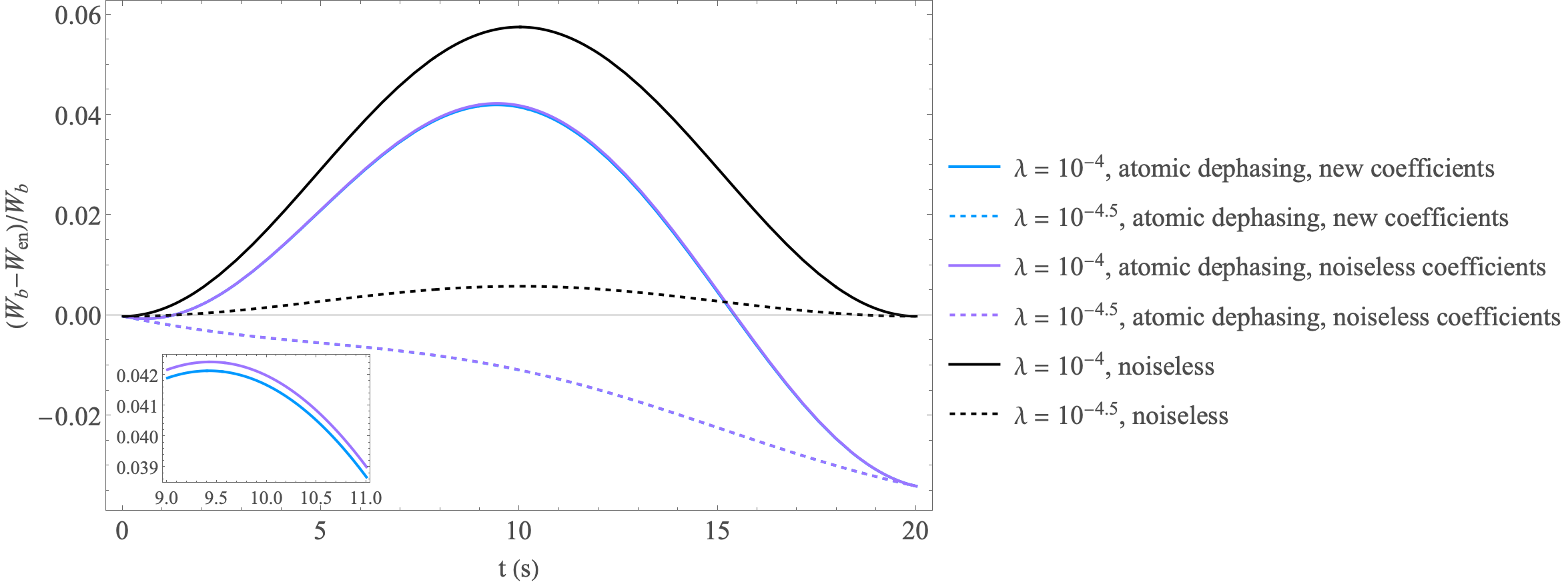
Note that the expressions are to ; , where is the coherence time of interferometer which we require to be large for interferometry; therefore, we expect . Here, we have used the same values of and as for the noiseless case. The difference between Equations 53 and 48 arises from dephasing-induced changes to the sum of the spin variances . If we break down the contributions from the different operators, we have
| (54) |
while the rest of the operators give
| (55) |
It can be seen that (given in Eq. 48), showing that atomic dephasing can make it harder to violate the separable-state bound. Since we used the same coefficients as for the noiseless case, the EW bound is partially given by of the noiseless case,
| (56) |
is the minimum value of the total spin variances for a separable state as can be experimentally achieved at the start of the experiment; its occurrence in this equation, which reduces the violation by , indicates the value we expect it to reduce to just before the measurement as atomic dephasing reduces the total quantum number.
We can further re-optimize the coefficients and for the case of dephasing by applying the constrain that . To and we have
| (57) | |||
| (58) | |||
| (59) | |||
| (60) |
Note that in the succeeding calculations, we used less simplified expressions; we do not present them here due to their complexity. As can be verified, these coefficients satisfy . The bound is now
| (61) |
The entangled-state value for the optimized coefficients remains the same as that of Eq. 53 to and ; that is, the “optimized” coefficients give the same entangled state value as when using noiseless coefficients (given in Eq. 53) to . Thus, we may as well use the noiseless coefficients for the case of atomic dephasing, because the “optimized” coefficients only serve to decrease while keeping unchanged.
I.1.4 Entanglement witness with a thermal state and white noise bath
We now elaborate on the case of thermal noise. There are three scenarios that can be considered; the first when the oscillator starts in a thermal state, the second when the oscillator starts in a thermal state and remains in contact with a white noise bath, and the third when the oscillator starts in the ground state and remains in contact with a bath.
For a thermal state [24]
| (63) |
introducing the initial-thermal-state-only effect into the previous noiseless calculation is rather straightforward. For average thermal occupancy , we need only replace the expectation values of any any and terms that appear in the evaluation of the Heisenberg picture operators as follows
| (64) | |||
| (65) |
We can then find the coefficients as listed in the main paper, along with the bound and entangled-state value .
Next, we consider the scenario where the oscillator is in continuous contact with a white noise bath. As explained in the main paper, we can solve for to obtain
| (66) |
With and , the noise contributions to and can be expressed as
| (67) | |||
| (68) |
Further, and will rotate about the z-axis by an angle as follows:
| (69) | |||
| (70) |
We can define the thermal noise contribution to this angle as
| (71) |
The covariances that contribute to the bath noise are as follows:
| (72) |
As examples, contributes to the noise in the EW term and contributes to the noise in . Therefore, the expectation values that compose the EW must be modified as shown in the main paper.
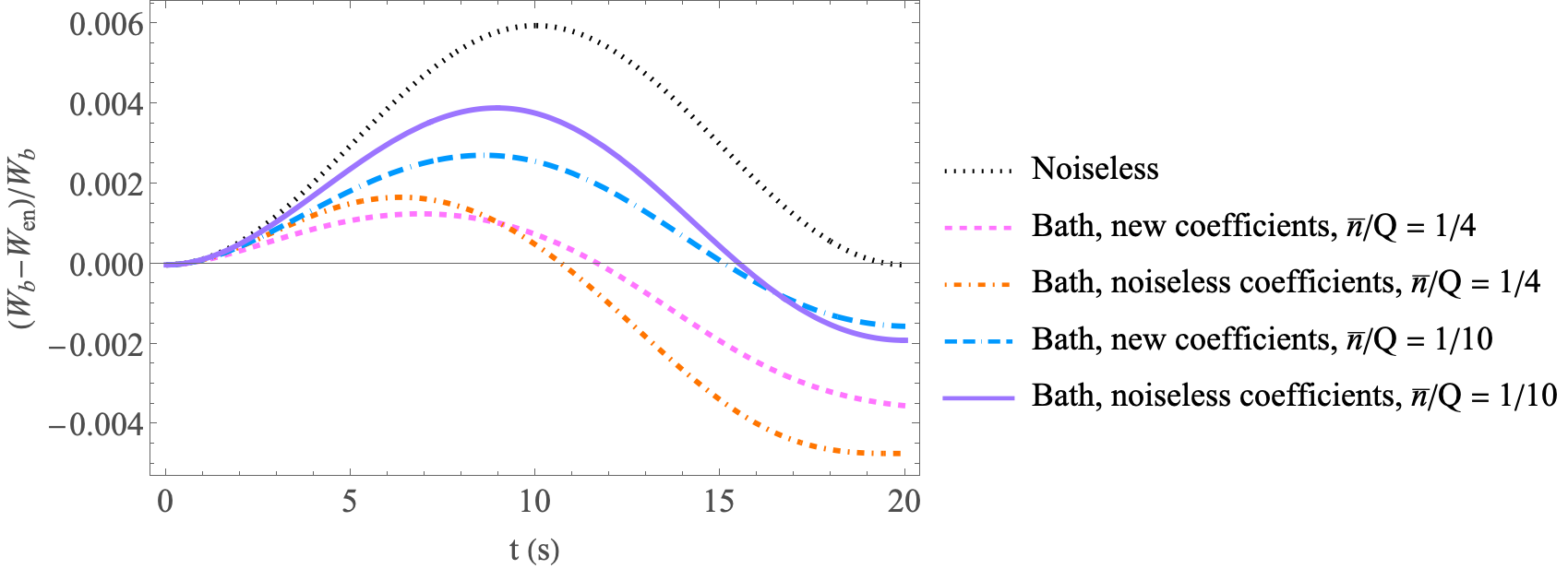
Next, we move to the scenario where the oscillator starts in a ground state and remains in contact with a white noise bath. Some additional plots to those in the main paper are shown in Fig. 4; in particular, plots for “re-optimized” coefficients. It can be seen that for certain values of , the re-optimized coefficients show higher violation for certain times than the noiseless coefficients, while for other values of , the noiseless coefficients are better.
I.2 Magnetic interactions
We now explain in detail the interaction between an atom interferometer and a mechanical oscillator, and how to the obtain the magnetic coupling between them.
Atom interferometers measure the phase difference accumulated by the components of an atom’s wave function that travel along different trajectories between two points in spacetime. In general, the phase accumulated by each component is the integral of the Lagrangian along the classical trajectory it traverses. In an optical lattice atom interferometer, the trajectories include a hold period where the atom is in a superposition of being trapped at different sites in an optical lattice. When this hold period is much longer than the time for the trajectories to separate and recombine, the dominant contribution to the relative phase is the integral of the force, , across the atoms at through the hold time, , multiplied by the atom separation . In units with , the interferometer phase has the following form [22]:
| (73) |
I.2.1 Interactions through the quadratic Zeeman effect
If the atoms are exposed to a spatially varying magnetic field, then a force across the atoms is generated due to the gradient in the Zeeman splitting of the atom’s energy levels. For Cesium-133 atoms in the ground state, the leading order Zeeman effect is quadratic in the magnetic field [25], yielding a force
| (74) |
Thus, atom interferometers can act as magnetometers, measuring the gradient in the magnitude of the magnetic field. If the source of the magnetic field is an oscillator composed of magnetic material, then the force across the atoms will encode the displacement of the oscillator, .
| (75) |
The atoms will feel a force that is modulated by the oscillator’s motion. This results in an interferometer phase that is sensitive to the oscillators position. There will also be a back action force on the oscillator, , from the dependence of the magnetic field on the oscillator’s position. This force will be sensitive to the atom’s position.
| (76) |
This physics is captured by the interaction potential for small displacements in the atom and oscillator coordinates.
| (77) |
The oscillator motion is now subject to a linear potential which modifies its motion and the potential interacts with the atoms, spatially separated by , to accumulate interferometer phase at a rate ,
| (78) |
Here, is an atom’s energy difference between the states of the ground state. To understand the magnitude of this interaction achievable with current technologies and how it can be increased, we model a particular experimental setup in the next section.
I.2.2 Proposed setup
| Parameter | Symbol | Value |
|---|---|---|
| Cs ground state shift [25] | 268.575 | |
| External magnetic field strength | mT | |
| magnetic susceptibility [29] | ||
| pendulum radius | 10 cm | |
| pendulum frequency | rad/s | |
| pendulum density [28] | 19.3 g/cm3 | |
| cylinder height | 10 mm | |
| cylinder radius | mm | |
| half of cylinder separation angle | ||
| atom to pendulum distance | 8 mm | |
| atom wave packet separation | 5 m |
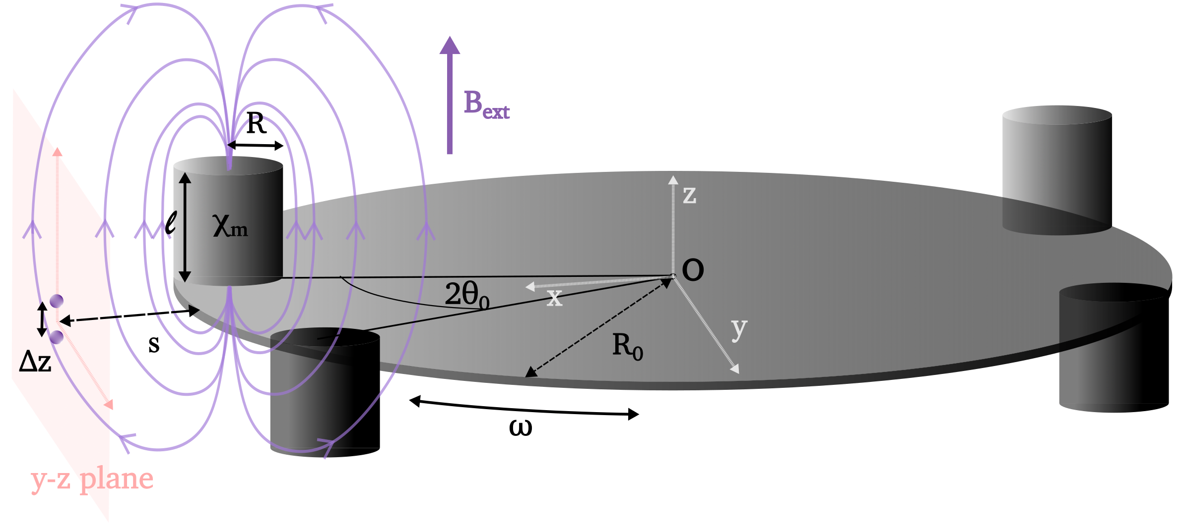
The main paper proposed a simplified version of the torsional pendulum. Since we plan to gradually proceed to a gravity experiment, we investigated a more advanced version of a pendulum as depicted in Figure 5. The pendulum that will oscillate at frequency about the vertical axis with two diamagnetic cylinders with magnetic susceptibility on its base. The atom interferometer sequence will trap atoms in a superposition of two lattice sites that are horizontally separated from the pendulum base by a distance, , and vertically separated above and below the base by ; that is, , since our atoms only have a vertical separation. In a uniform external magnetic field, , these cylinders will produce an induced magnetic field. The gradients in the induced field will couple to the atom interferometer through the quadratic Zeeman effect to produce an interaction potential that is sensitive to the pendulum’s rotation angle and the atom’s location.
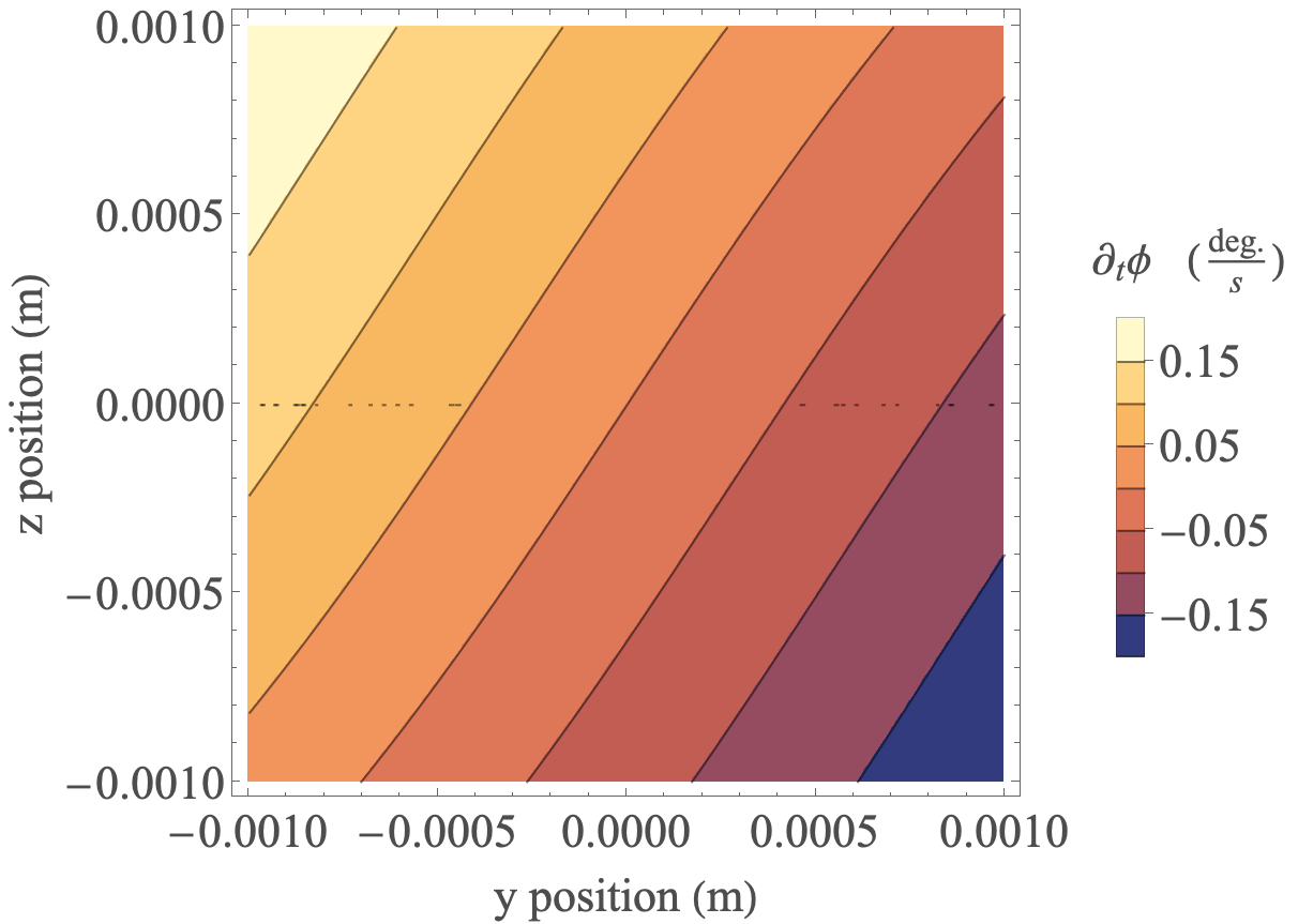
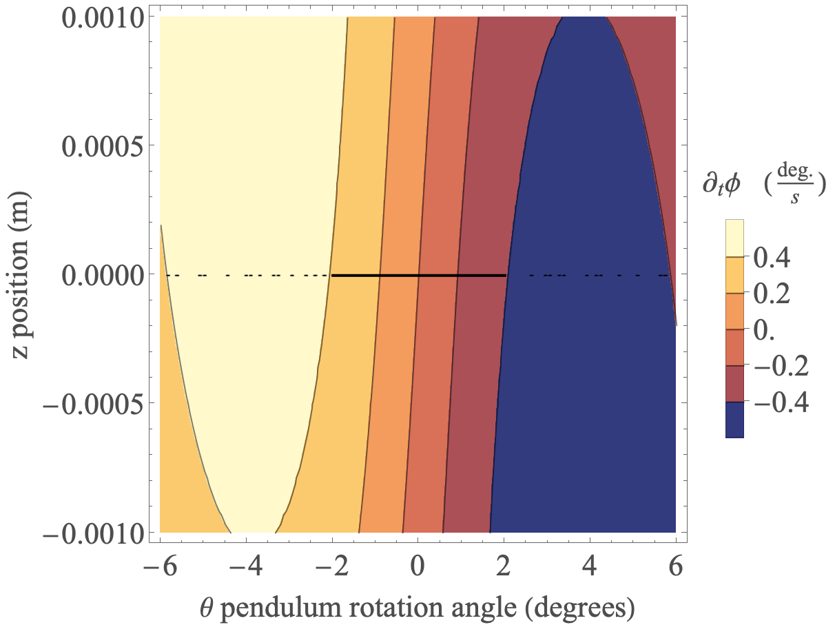
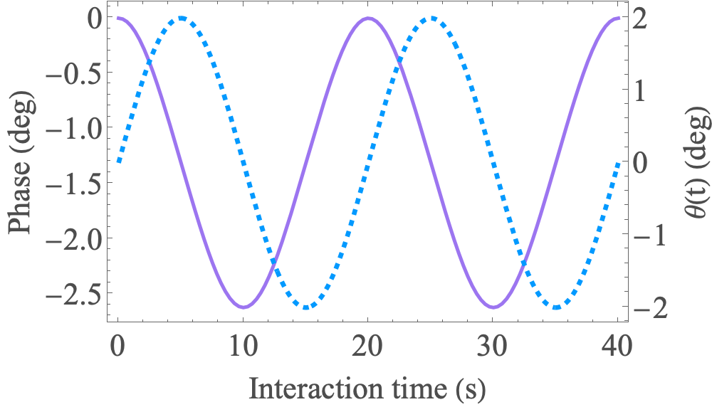
The magnetic field from a finite length cylinder with uniform magnetization has been calculated in Ref. [27]. The total magnetic field is a superposition of the induced field from each cylinder and the external magnetic field. The resulting phase accumulation rate for a range of atom locations and oscillator rotation angles is displayed in Figures 6a and 6b. With the atoms centered at , the interferometer phase is calculated for the oscillator in classical motion: . The result is plotted in Fig. 7 along with the rotation angle of the oscillator. The interferometer phase, and therefore the probability to find the atom in each lattice site, is clearly correlated with the oscillators position. If the oscillator is quantum mechanical and its position and momentum become sufficiently correlated with the atoms, then there is the possibility of observing the system in a non-classical state.
I.2.3 Interaction with a quantum harmonic oscillator
The combined oscillator-atom Hamiltonian has the following form [18]:
| (79) |
Here, and are the oscillator creation and annihilation operators, while is a pseudo-spin operator describing the atom’s location. The second term is the interaction potential in Eq. 77 with quantized oscillator and atom coordinates. is defined as follows.
| (80) |
Here, is the number of cylinders. The factor of simply arises from taking the derivative in the direction of . For oscillator mass and frequency and , the harmonic oscillator position operator is . Since the atom is confined to two sites in an optical lattice separated by , the atom’s position operator can be expressed as a spin operator in a pseudo-spin-1/2 Hilbert space.
| (81) |
For the more realistic case of an atom interferometer with atoms, the interaction potential can be linearized in each of their coordinates to produce an interaction linear in the collective pseudo-spin operator [18].
| (82) |
The system Hamiltonian, Eq. 79, is capable of generating entanglement between the atoms and oscillator. For the oscillator initialized in its ground state and the atom in a symmetric spatial superposition, the system evolves to an entangled state where the displacement of the oscillator is correlated with the atom’s location [18],
| (83) |
is the coherent state amplitude proportional to . For an experiment to resolve the correlations between the oscillator and the atom, must be sufficiently large.
We can readily calculate with Eq. 80 for our proposed setup. With the parameter values in Table 1, we find the following value for (for = 4) to first order in :
| (84) |
The susceptibility of and density of correspond to those of tungsten [28, 29]. parametrizes the length scale of the system as ; that is, is the scaling factor for all the length parameters in Table 1, with the exception of (i.e the parameters and ). This scaling implies that is increased by decreasing the system size. In the parameter space we are at, recalling that (with being the induced magnetic field of the cylinders), the term of Eq. 80 can be approximated to be . This is because has no gradient and is negligible compared to the cross-term. This allows the scalings of and to be expressed as “single” factors. As a side note, the value of was obtained using the expressions in Ref. [27].
The value of the coupling in Eq. 80 is extremely small. As will be seen in the succeeding sections, entanglement witness violation requires couplings of around , which is orders of magnitude larger than that which can be obtained from the parameters in Table 1. There are several ways through which we can increase . One of the primary changes is to switch to a superconducting mass. Though one might think that this will re-introduce the contribution from , it is still smaller than the cross-term (at least for the physical parameters we use). Therefore, we can still use Eq. 80 to inform us of how the values change with rescaling the parameters; having said that, the upcoming calculation was done exactly using the expressions in Ref. [27]. We now have , which will increase the coupling by a factor of ; increasing the field to 50 mT will contribute a factor of (note that at this field, we are still well before the Paschen-Back regime for cesium, as seen in Ref. [25]); the system size can be reduced by a factor of 2 (taking ); a cloud of atoms leads to a increase - we set . If we take the material to be lead, then the density will be g/cm3 [26]. Together, these factors increase the coupling to . The main concern would be the experimental challenges for some of these changes; in particular, scaling the atom to pendulum distance from 8 mm to 4 mm would be pushing the limits of existing systems, since there is a requirement that the atom trap laser not interact with the pendulum.
We can also gain improvements in coupling by having the cesium atoms be magnetically sensitive states; for instance, we can place one atom in the state and the other in the . In such a scenario, the coupling would primarily be due to the first order Zeeman shift, which is linear in [25]. The energy difference in the atoms now arises due to the difference in their internal states, in addition to the magnetic field differences between their two locations (that is, a coupling will exist even if ). In particular, the term of the Zeeman energy shift which contributes to the coupling is [25]
| (85) |
where is the nuclear spin, which is 7/2 for Cs; we take the difference of this quantity between the two atoms, and then the gradient in the direction of oscillator motion to obtain the coupling. However, having atoms be located symmetrically in the top and bottom halves of the cylinder is detrimental to the coupling, because now it arises solely from . Thus, we shift the positions of both atoms such that they are both in plane. If we place the top atom to be at around , we obtain the coupling to be
| (86) |
we can see that it is now four orders of magnitude higher. Note that the scaling here also incorporates changing the position of the top atom location by a factor of ; the separation between the two atom locations is still kept constant, so the position of the second location changes too. For 50 mT, , g/cm3 [26], , and , we will get , which is a significant improvement from having purely states. Note that scaling also decreases the atom-oscillator separation from 8 mm to 4 mm.
If we re-calculate the superconducting case for the simplified setup in the main paper, with changes such that , the atom-oscillator separation is 8 mm (which is the more feasible situation), and the atoms are symmetrically located at , we get (as quoted in the main paper). Potential issues of having the atoms be in magnetically sensitive states is that it can introduce sensitivities to stray magnetic fields.
References
- Kong et al. [2020] J. Kong, R. Jiménez-Martínez, C. Troullinou, V. G. Lucivero, G. Tóth, and M. W. Mitchell, Measurement-induced, spatially-extended entanglement in a hot, strongly-interacting atomic system, Nat. Commun. 11, 2415 (2020).
- Bose et al. [2017] S. Bose, A. Mazumdar, G. W. Morley, H. Ulbricht, M. Toroš, M. Paternostro, A. A. Geraci, P. F. Barker, M. S. Kim, and G. Milburn, Spin entanglement witness for quantum gravity, Phys. Rev. Lett. 119, 240401 (2017).
- Bartling et al. [2022] H. P. Bartling, M. H. Abobeih, B. Pingault, M. J. Degen, S. J. H. Loenen, C. E. Bradley, J. Randall, M. Markham, D. J. Twitchen, and T. H. Taminiau, Entanglement of spin-pair qubits with intrinsic dephasing times exceeding a minute, Phys. Rev. X 12, 011048 (2022).
- Bai et al. [2017] X.-M. Bai, C.-P. Gao, J.-Q. Li, N. Liu, and J.-Q. Liang, Entanglement dynamics for two spins in an optical cavity – field interaction induced decoherence and coherence revival, Opt. Express 25, 17051 (2017).
- Rosenfeld et al. [2021] E. Rosenfeld, R. Riedinger, J. Gieseler, M. Schuetz, and M. D. Lukin, Efficient entanglement of spin qubits mediated by a hot mechanical oscillator, Phys. Rev. Lett. 126, 250505 (2021).
- Ockeloen-Korppi et al. [2018] C. F. Ockeloen-Korppi, E. Damskägg, J.-M. Pirkkalainen, M. Asjad, A. A. Clerk, F. Massel, M. J. Woolley, and M. A. Sillanpää, Stabilized entanglement of massive mechanical oscillators, Nature 556, 478–482 (2018).
- Riedinger et al. [2018] R. Riedinger, A. Wallucks, I. Marinković, C. Löschnauer, M. Aspelmeyer, S. Hong, and S. Gröblacher, Remote quantum entanglement between two micromechanical oscillators, Nature 556, 473–477 (2018).
- Bengyat et al. [2024] O. Bengyat, A. Di Biagio, M. Aspelmeyer, and M. Christodoulou, Gravity-mediated entanglement between oscillators as quantum superposition of geometries, Phys. Rev. D 110, 056046 (2024).
- Liu et al. [2024] J.-X. Liu, J.-Y. Yang, T.-X. Lu, Y.-F. Jiao, and H. Jing, Phase-controlled robust quantum entanglement of remote mechanical oscillators, Phys. Rev. A 109, 023519 (2024).
- Kao and Chou [2016] J.-Y. Kao and C.-H. Chou, Quantum entanglement in coupled harmonic oscillator systems: from micro to macro, New J. Phys. 18, 073001 (2016).
- Laha et al. [2022] P. Laha, L. Slodička, D. W. Moore, and R. Filip, Thermaly induced entanglement of atomic oscillators, Opt. Express 30, 8814 (2022).
- Jellal et al. [2011] A. Jellal, F. Madouri, and A. Merdaci, Entanglement in coupled harmonic oscillators studied using a unitary transformation, J. Stat. Mech. 2011, P09015 (2011).
- Thomas et al. [2021] R. A. Thomas, M. Parniak, C. Østfeldt, C. B. Møller, C. Bærentsen, Y. Tsaturyan, A. Schliesser, J. Appel, E. Zeuthen, and E. S. Polzik, Entanglement between distant macroscopic mechanical and spin systems, Nat. Phys. 17, 228 (2021).
- Monroe et al. [1995] C. Monroe, D. M. Meekhof, B. E. King, W. M. Itano, and D. J. Wineland, Demonstration of a fundamental quantum logic gate, Phys. Rev. Lett. 75, 4714 (1995).
- Lo et al. [2015] H.-Y. Lo, D. Kienzler, L. de Clercq, M. Marinelli, V. Negnevitsky, B. C. Keitch, and J. P. Home, Spin–motion entanglement and state diagnosis with squeezed oscillator wavepackets, Nature 521, 336–339 (2015).
- Kafri and Taylor [2013] D. Kafri and J. M. Taylor, A noise inequality for classical forces (2013), arXiv:1311.4558 [quant-ph] .
- Marletto and Vedral [2017] C. Marletto and V. Vedral, Gravitationally induced entanglement between two massive particles is sufficient evidence of quantum effects in gravity, Phys. Rev. Lett. 119, 240402 (2017).
- Carney et al. [2021] D. Carney, H. Müller, and J. M. Taylor, Using an Atom Interferometer to Infer Gravitational Entanglement Generation, PRX Quantum 2, 030330 (2021).
- Bell [1964] J. S. Bell, On the Einstein Podolsky Rosen paradox, Physics Physique Fizika 1, 195 (1964).
- Gühne and Tóth [2009] O. Gühne and G. Tóth, Entanglement detection, Physics Reports 474, 1 (2009).
- Duan et al. [2000] L.-M. Duan, G. Giedke, J. I. Cirac, and P. Zoller, Inseparability criterion for continuous variable systems, Phys. Rev. Lett. 84, 2722 (2000).
- Xu et al. [2019] V. Xu, M. Jaffe, C. D. Panda, S. L. Kristensen, L. W. Clark, and H. Müller, Probing gravity by holding atoms for 20 seconds, Science 366, 745 (2019).
- Hofmann and Takeuchi [2003] H. F. Hofmann and S. Takeuchi, Violation of local uncertainty relations as a signature of entanglement, Phys. Rev. A 68, 032103 (2003).
- [24] Quantum states of light, http://www.quantum.physik.uni-potsdam.de/teaching/ws2009/qo1/script-ch34.pdf.
- Steck [1998] D. A. Steck, Cesium D Line Data, website (1998), revision 1.6, Oct 2003.
- [26] PubChem Compound Summary for CID 5352425, Lead, online, National Center for Biotechnology Information.
- Caciagli et al. [2018] A. Caciagli, R. J. Baars, A. P. Philipse, and B. W. Kuipers, Exact expression for the magnetic field of a finite cylinder with arbitrary uniform magnetization, Journal of Magnetism and Magnetic Materials 456, 423 (2018).
- [28] PubChem Compound Summary for CID 23964, Tungsten, online, National Center for Biotechnology Information.
- Fitzpatrick [2006] R. Fitzpatrick, Magnetic susceptibility and permeability, online (2006).