Entanglement between charge qubit states and coherent states of nanomechanical resonator generated by AC Josephson effect

Electro-mechanical phenomena on the nanometer scale attract significant attention during the last two decades. Roukes Recent advantages in nanotechnologies acquire a promising platform for studying the fundamental phenomena generated by the interplay between quasi-classical and pure quantum subsystems. A charge qubit formed by a tiny superconducting island (Cooper-pair box (CPB)) whose basis states are charge states (e.g. states which represent the presence or absence of excess Cooper pairs on the island), is one of a large group of pure quantum systems. Pashkin At the same time modern nanomechanical resonators which dynamics according to Ehrenfest theorem to great extent is described by classical equations, are ideal representatives of quasiclassical subsystem Schmid . Systems, which dynamics is determined by the mutual influence between a superconducting qubit and a nanomechanical resonator, are a subject of cutting-edge research in quantum physics, especially, in quantum communication, see, e.g., Refs. Cleland1 ; Cleland2 ; Chu ; Cleland3 ; LaH ; Tian

There are two main questions that arise related to an interplay between quasi-classical dynamics of the mechanical resonator and quantum dynamics of the charge qubit. The first one is: how quasi-classical motion may affect pure quantum phenomena? Considering this question, it was shown that the superconducting current between two remote superconductors can be established by mechanical transportation of Cooper pairs performed by an oscillating CPB. Gorelik2 Even more, it was demonstrated that such transportation may generate correlations between the phases of space-separated superconductors. Isacsson Another question is how coherent Josephson dynamics of a charge qubit will affect the dynamics of the quasi-classical resonator, in particular, whether or not the quantum entanglement between a superconducting qubit and mechanical vibrations can be achieved? Recently it was demonstrated that individual phonons can be controlled and detected by a superconducting qubit enabling coherent generation and registration of quantum superposition of zero and one-phonon Fock states Cleland1 ; Cleland2 . At the same time nanomechanical resonators provide the possibility to store quantum information in the complex multi-phonon coherent states. Such states, in contrast to single-phonon states, where mechanical losses irreversibly delete the quantum information, allow their detection and correction Girvin ; Girvin1 . Motivated by such a challenge, in this paper, we demonstrate the possibility to generate quantum entanglement between the charge qubit states and mechanical coherent ones in a particular nanoelectromechanical system (NEMS) where mechanical vibrations are highly affected due to the weak coupling with movable a Cooper-pair box.

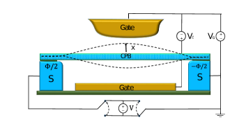
Schematic representation of the NEMS prototype considered in this article is presented in Fig. 1. It consists of the superconducting nanowire (SCNW),NW1 ; NW2 , which is suspended between two bulk superconductors and is capacitively coupled to the two side gate electrodes. In this paper, we will consider the case when SCNW represents a superconducting island that can be treated as a charge qubit (Cooper-pair box) whose basis states are charge states - states which represent the presence or absence of excess Cooper pairs on the island. Below we will refer to these states as charge and neutral states correspondingly. As this takes place, the gate voltage $V_{G}$ and the voltage applied between the gates $V_{\mathcal{E}}$ are chosen in a way that the difference in the electrostatic energies of the charged and neutral states equals to zero at the straight configuration of the nanowire, while nanowire bending removes this degeneracy. We also reduce the bending dynamics of the SCNW to the dynamics of the fundamental flexural mode described by the harmonic oscillator.

Joint Cooper pairs dynamics and mechanical one of this system is described by the Hamiltonian which can be presented in the form,

			$\displaystyle H=H_{q}+H_{m}+H_{int},$
			$\displaystyle H_{q}=-E_{J}\sigma_{1}\cos\Phi,\quad H_{m}=\frac{\hbar\omega}{2}\left(\hat{x}^{2}+\hat{p}^{2}\right),$
			$\displaystyle H_{int}=\varepsilon\hat{x}\sigma_{3}.$

Here Hamiltonian $H_{q}$ represents Josephson coupling between CPB and bulk superconductors. The constant $E_{J}$ is the Josephson coupling energy (in this paper we will consider only the case of symmetric coupling), $\Phi=\Phi(t)$ is the superconducting phase difference between electrodes, $\sigma_{i}(i=1,2,3)$ are the Pauli matrices acting in the qubit Hilbert space in a basis where vectors $(1,0)^{T}$ and $(0,1)^{T}$ represent charged and neutral states, respectively. Hamiltonian $H_{m}$ in Eq. (Model and Hamiltonian) represents dynamics of the fundamental bending mode described by the harmonic oscillator with frequency $\omega$ (here momentum and coordinate operators, $\hat{p}$ and $\hat{x}$, are normalized on the amplitude of zero-point oscillations $x_{0}=\sqrt{\hbar/M\omega}$, $M$ is an effective mass, $[\hat{x},\hat{p}]=\imath$). The third term, $H_{int}$, describes an electromechanical coupling between the charge qubit and the mechanical oscillator induced by the electrostatic force acting on the charged state of the qubit, $\varepsilon=e\mathcal{E}x_{0}$. In the last equality, $\mathcal{E}$ is an effective electrostatic field that is controlled by the difference of the applied voltages $V_{G}$ and $V_{\varepsilon}$. Below we will assume $\varepsilon\ll\hbar\omega,E_{J}$ that corresponds to the typical experimental situation.Cleland1 ; Tian ; A-A

The states of the system described by the Hamiltonian, Eq. (Model and Hamiltonian), are a superposition of direct products of qubit states, $\mathbf{e}^{\pm}_{i}$, and eigenstates of the oscillator $|n\rangle$ (here and below $\mathbf{e}^{\kappa}_{i}$ denotes the eigenvectors of the Pauli matrices $\sigma_{i}$ with eigenvalues $\kappa=\pm 1$).

If $\varepsilon=0$, the interaction between the qubit and the mechanical subsystem is switched off and stationary states of the Hamiltonian, Eq. (Model and Hamiltonian), are pure states (the entropy of entanglement is an integral of motion, i.e. if the system is initially, in a pure state, it will be in a pure state at any moment of time). Synchronous switching on the electrical field $\mathcal{E}$ and the bias voltage between superconducting leads ($\dot{\Phi}(t)=2eV/\hbar$) results in the evolution of such pure states in the states represented by entanglement between the qubit and oscillator states.

To carry out an analysis of this evolution, we introduce the dimensionless time and energies, $\omega t\rightarrow t,E_{J}/\hbar\omega\rightarrow E_{J},\varepsilon/\hbar\omega\rightarrow\varepsilon$ and assume that at the moment of switching on the interaction between the subsystems ($t=0$), the difference between the superconducting phases is $\Phi=\Phi_{0}$ and the system has been in a pure state,

$$|\Psi(0)\rangle=\mathbf{e}_{in}\otimes|0\rangle.$$

(2)

At $t>0$ according to Josephson relation $\Phi(t)=2eVt/\hbar\omega+\Phi_{0}$. The Hamiltonian, Eq. (Model and Hamiltonian), and, as a consequence, the time evolution operator $\hat{U}(t,t^{\prime})$, which is defining evolution of the arbitrarily initial state, has the properties:

$$\hat{H}(t+T_{V})=\hat{H}(t),\quad\hat{U}(t,t^{\prime})=\hat{U}(t+T_{V},t^{\prime}+T_{V}),$$

(3)

where $T_{V}=2\pi/\Omega_{V}=\pi\hbar\omega/e|V|$. To analyze the evolution operator, one can use the interaction picture taking

$$\hat{U}(t,t^{\prime})=\hat{\mathcal{U}}_{\eta}(t)\hat{\mathcal{U}}_{\eta}(t,t^{\prime})\hat{\mathcal{U}}^{\dagger}_{\eta}(t^{\prime}),$$

(4)

where

$$\hat{\mathcal{U}}_{\eta}(t)=\exp\left[\frac{\imath E_{J}}{\Omega_{V}}\sigma_{1}\sin\left(\Omega_{V}t+\eta\Phi_{0}\right)-\imath a^{\dagger}at\right].$$

(5)

The parameter $\eta=\text{sgn}\left(V/|V|\right)=\pm$ characterizes the direction of the bias voltage drop. The operator $\hat{\mathcal{U}}_{\eta}(t,t^{\prime})$ obeys the following equation:

	$\displaystyle\imath\frac{\partial\hat{\mathcal{U}}_{\eta}(t,t^{\prime})}{\partial t}=\hat{\mathcal{H}}_{\eta}(t)\hat{\mathcal{U}}_{\eta}(t,t^{\prime}),$
	$\displaystyle\hat{\mathcal{H}}_{\eta}(t)=\varepsilon\hat{x}(t)\sigma_{3}(t),\quad\hat{\mathcal{U}}_{\eta}(t,t)=\hat{I}.$		(6)

Here

	$\displaystyle\hat{x}(t)=\frac{1}{\sqrt{2}}(\hat{a}\text{e}^{-\imath t}+\hat{a}^{\dagger}\mathrm{e}^{\imath t}),$
	$\displaystyle\sigma_{3}(t)=\sigma_{3}\cos\left(\frac{E_{J}}{\Omega_{V}}\sin(\Omega_{V}t+\eta\Phi_{0})\right)-$
	$\displaystyle\hskip 28.45274pt-\sigma_{2}\sin\left(\frac{E_{J}}{\Omega_{V}}\sin(\Omega_{V}t+\eta\Phi_{0})\right).$		(7)

If the frequencies $\omega$ and $\Omega_{V}$ are incommensurable, the operator $\hat{\mathcal{H}}_{\eta}(t)$ is a quasiperiodic function of time. In such a case one can expect that the mechanical subsystem, being initially in the ground state, does not significantly deviate from this state in the process of evolution. However, a rigorous consideration of this case requires independent research and will be done elsewhere. In this paper, we will consider the resonant case when $\Omega_{V}=\omega$ and will assume that $\varepsilon\ll 1$. The first condition stipulates the following properties of the evolution operator,

$$\hat{\mathcal{U}}_{\eta}(2\pi N,2\pi N^{\prime})=\left(\hat{\mathcal{U}}_{\eta}(2\pi,0)\right)^{N-N^{\prime}},$$

(8)

where $N,N^{\prime}$ are the natural numbers. The second assumption allows us to make the following substitution in a leading approximation regarding small $\varepsilon$,

$$\hat{\mathcal{U}}_{\eta}(t,t^{\prime})=\hat{\mathcal{U}}_{\eta}(2\pi N,2\pi N^{\prime}),$$

(9)

where $N(N^{\prime})=[t(t^{\prime})/2\pi]([x]$ is an integer part of $x$), and obtain an expression for $\hat{\mathcal{U}}_{\eta}(2\pi,0)$ which can be written as,

	$\displaystyle\hat{\mathcal{U}}_{\eta}(2\pi,0)=\exp\left[\imath\tilde{\varepsilon}\sigma_{2}\hat{p}(\eta\Phi_{0})+\varepsilon^{2}{\cal O}(\hat{I})\right],$
	$\displaystyle\hat{p}(\Phi)=\hat{p}\cos\Phi+\hat{x}\sin\Phi.$		(10)

Here $\tilde{\varepsilon}=2\pi\varepsilon J_{1}(2E_{J})$ and $J_{1}(x)$ the Bessel function of the first kind. Using the above relations one can obtain an expression for the evolution operator $\hat{U}(t,t^{\prime})$, which in the main approximation regarding $\varepsilon$ has a form,

$$\hat{U}(t,t^{\prime})=\hat{\mathcal{U}}_{\eta}(t)\exp\left[\imath\tilde{\varepsilon}\sigma_{2}\hat{p}(\eta\Phi_{0})(t-t^{\prime})\right]\hat{\mathcal{U}}^{\dagger}_{\eta}(t^{\prime}).$$

(11)

Using Eqs. (2),(11) one gets that at the time $t$, with the accuracy to small parameter $\tilde{\varepsilon}\ll 1$, the state of the system $|\Psi(t)\rangle$ is given by an expression,

$$|\Psi(t)\rangle=\sum\limits_{\kappa}A_{\kappa}^{\eta}\mathbf{e}^{\kappa}_{2}(t,\eta\Phi_{0})\otimes|-\kappa\mathrm{z}(t,\eta)/\sqrt{2}\rangle.$$

(12)

Here

$$\mathbf{e}^{\kappa}_{2}(t,\eta\Phi_{0})=\mathbf{e}^{\kappa}_{2}\exp\left[\imath E_{J}\sigma_{1}\sin(t+\eta\Phi_{0})\right]$$

and $\mathbf{e}_{2}^{\kappa}=\sigma_{1}\mathbf{e}_{2}^{-\kappa}$ are the eigenvectors of Pauli matrix $\sigma_{2}$ with eigenvalues $\kappa=\pm 1,A_{\kappa}^{\eta}=\left(\mathbf{e}_{2}^{\kappa}(0,\eta\Phi_{0}),\mathbf{e}_{in}\right)$. The symbol $|\alpha\rangle$ (where $\alpha$ is a complex number) denotes the coherent states of the oscillator, $\hat{a}|\alpha\rangle=\alpha|\alpha\rangle$, while a complex function $\mathrm{z}(t,\eta)$ is defined as

$$\mathrm{z}(t,\eta)=\tilde{\varepsilon}t\exp\left[-\imath(t+\eta\Phi_{0})\right].$$

(13)

It should be stressed that Eq. (12) is valid only for restricted time interval $t\leq\tilde{\varepsilon}^{-2}$. Time $t$ should be also shorter than any dephasing and relaxation times. From Eq. (12) one can see that initially pure state $|\Psi(t=0)\rangle=\mathbf{e}_{in}\otimes|0\rangle$ evolves into the state represented by the entanglement between the two qubit states and two coherent states of the mechanical resonator. Moreover, the details of this entanglement depend on switching time (parameter $\Phi_{0}$) and direction of the bias voltage (parameter $\eta$). These circumstances allow one to manipulate the described above entanglement by switching the bias voltage direction.

To demonstrate the effect of the entanglement between the charge qubit and mechanical vibrations that comprehends the formation of so-called Schrödinger-cat states of nanomechanical resonator, we consider the following time protocol for $V(t)$:

$$2eV(t)=-\hbar\omega\theta(t)\left[1-2\theta(t-t_{s})\right].$$

Namely, during the time interval $0<t<t_{s}$ the bias voltage $V(t)=-\hbar\omega/2e$ and then it switches its sign. Using Eqs. (4), (8), (Time evolution), one gets that at $t>t_{s}$,

	$\displaystyle\hat{U}(t,0)=\hat{\mathcal{U}}_{+}(t)\text{e}^{\imath\sigma_{2}\tilde{\varepsilon}(t-t_{s})\hat{p}(\Phi_{0})}\hat{S}\text{e}^{\imath\sigma_{2}\tilde{\varepsilon}t_{s}\hat{p}(-\Phi_{0})}\hat{\mathcal{U}}_{-}(0),$
	$\displaystyle\hat{S}=\hat{\mathcal{U}}_{+}^{\dagger}(t_{s})\hat{\mathcal{U}}_{-}(t_{s})\equiv\rho(t_{s},\Phi_{0})+\imath\tau(t_{s},\Phi_{0})\sigma_{1},$		(14)
	$\displaystyle\rho(t_{s},\Phi_{0})=\cos\left(2E_{J}\cos t_{s}\sin\Phi_{0}\right),$
	$\displaystyle\tau(t_{s},\Phi_{0})=-\sin\left(2E_{J}\cos t_{s}\sin\Phi_{0}\right).$

As a result, the state of the system after changing the direction of the bias voltage has a form:

	$\displaystyle|\Psi(t)\rangle=\sum\limits_{\kappa}\mathbf{e}^{\kappa}_{2}(t,\Phi_{0})\otimes$
	$\displaystyle\otimes\left(\rho A_{\kappa}^{-}|-\kappa\mathrm{z}_{+}/\sqrt{2}\rangle+\imath\tau A_{-\kappa}^{-}|\kappa\mathrm{z}_{-}/\sqrt{2}\rangle\right),$		(15)

where $\mathrm{z}_{\pm}=\mathrm{z}_{1}\pm\mathrm{z}_{2}$ and

$$\mathrm{z}_{1}=\text{e}^{-\imath(t-\Phi_{0})}\tilde{\varepsilon}t_{s},\mathrm{z}_{2}=\text{e}^{-\imath(t+\Phi_{0})}\tilde{\varepsilon}(t-t_{s})$$

(16)

(see Fig. 2). It can be seen from this equation that the state of the system is represented by the entanglement of two qubit’s state with two so-called “cat-states” (superposition of coherent states) whose structure is controlled by the parameters $E_{J}\ (\rho)$ and $\Phi_{0}$. As it follows from Eqs. (Generation of “cat-states”), (16), the bias voltage switching does not affect the dynamics of the system if $\Phi_{0}=0,\pi$.

Below we will limit ourselves to considering a most interesting, from our point of view, case when $\Phi_{0}=\pi/2$ and put $\mathbf{e}_{in}=(\mathbf{e}_{2}^{+}+\mathbf{e}^{-}_{2})/\sqrt{2}$, that is, we suppose that immediately before the interaction was switched on, the qubit was in the eigenstate of the operator $\hat{H}_{q}(t=0-\delta)$. These assumptions lead to the following relations $A_{+}^{-}=A_{-}^{-}=\exp(\imath E_{J})/\sqrt{2}$ in Eq. (Generation of “cat-states”). To characterize the entanglement between the qubit states and the states of the mechanical oscillator, we introduce the reduced density matrices, $\hat{\varrho}_{q(m)}(t)=\mathrm{Tr}_{m(q)}\hat{\varrho}$, where $\hat{\varrho}=|\Psi(t)\rangle\langle\Psi(t)|$ is a complete density matrix of the system and $\mathrm{Tr}_{m(q)}$ denotes the trace over mechanical (qubit) degrees of freedom. Using Eqs.  (12,Generation of “cat-states”), one can get the following expression for the $\hat{\varrho}_{q}$,

$$\hat{\varrho}_{q}(t)=\frac{I+\lambda(t,t_{s})\sigma_{1}}{2},$$

(17)

where

	$\displaystyle\lambda(t,t_{s})=\exp{\left(-\tilde{\varepsilon}^{2}t^{2}\right)},\hskip 28.45274pt0<t\leq t_{s},$		(18)
	$\displaystyle\lambda(t,t_{s})=\rho^{2}\exp{\left[-\tilde{\varepsilon}^{2}(t-2t_{s})^{2}\right]}+$
	$\displaystyle\hskip 34.14322pt+\tau^{2}\exp{\left(-\tilde{\varepsilon}^{2}t^{2}\right)},\hskip 36.98866ptt>t_{s}.$		(19)

In deriving this equation, we took into account relation $\mathbf{e}_{2}^{+}\cdot\mathbf{e}_{2}^{-}+\mathbf{e}_{2}^{-}\cdot\mathbf{e}_{2}^{+}=\sigma_{1}$. Using Eq. (17) one can calculate the entropy of entanglement,

$$S_{en}(t)\equiv-\operatorname{Tr}\hat{\varrho}_{q}(t)\log\widehat{\varrho}_{q}(t)=-\operatorname{Tr}\hat{\varrho}_{m}(t)\log\widehat{\varrho}_{m}(t).$$

(20)

One can find that $S_{en}(t)$ monotonically increases in time within intervals $0<t<t_{s}$ and $2t_{s}<t<\infty$ saturating to the maximal value $S_{en}^{\text{(max)}}=\log 2$ at $t\rightarrow\infty$. Within interval $t_{s}<t\leq 2t_{s}$ the behavior of the entanglement entropy depends on the relation between $\rho$ and $\tau$. In particular, for $\rho^{2}>\tau^{2}$ the entanglement entropy $S_{en}(t)$ starts to decrease after switching, reaching some minimal value (equals zero for the $\rho^{2}=1$) within interval $t_{s}<t\leq 2t_{s}$. If $\rho^{2}<\tau^{2}$, the entropy continues to grow just after the switching. However, its derivative might be also negative within some time interval whose existence is controlled by the parameters $\tilde{\varepsilon}t_{s}$ and $\tau^{2}/\rho^{2}$. The plot of $S_{en}(t)$ for $\tilde{\varepsilon}t_{s}=1$ and different values of $\rho$ is presented in Fig. 3.

———————————————————————–

To describe the evolution of the mechanical subsystem, we consider the reduced density matrix $\widehat{\varrho}_{m}(t)$. From Eq. (Generation of “cat-states”) one gets that at $t>t_{s}$:

	$\displaystyle\hat{\varrho}_{m}(t)=$
	$\displaystyle\frac{1}{2}\sum\limits_{\kappa}\left[\rho^{2}|\kappa\mathrm{z}_{+}/\sqrt{2}\rangle\langle\kappa\mathrm{z}_{+}/\sqrt{2}|+\tau^{2}|\kappa\mathrm{z}_{-}/\sqrt{2}\rangle\langle\kappa\mathrm{z}_{-}/\sqrt{2}|-\right.$
	$\displaystyle\left.-\imath\rho\tau\left(|-\kappa\mathrm{z}_{+}/\sqrt{2}\rangle\langle\kappa\mathrm{z}_{-}/\sqrt{2}|-\text{H.c.}\right)\right].$		(21)

To visualize the state of the mechanical subsystem, it is convenient to use the Wigner function representation for the density matrix $\hat{\varrho}_{m}(t)$,

$$W(x,p,t)=\frac{1}{\pi}\int\varrho_{m}(x+y,x-y,t)\exp(2\imath py)dy,$$

where $\varrho_{m}(x,x^{\prime},t)=\langle x|\hat{\varrho}_{m}(t)|x^{\prime}\rangle$. Using Eq. (Evolution of mechanical subsystem and average current), one gets,

$$W(x,p,t)=W_{t}(x\cos t-p\sin t,p\cos t+x\sin t),$$

(22)

where the function $W_{t}(x,p)$ is defined according to the relation,

	$\displaystyle W_{t}(x,p)=$
	$\displaystyle\frac{1}{2}\sum\limits_{\kappa}\left[\rho^{2}W_{0}(x,p+\kappa|\mathrm{z}_{+}|)+\tau^{2}W_{0}(x,p-\kappa|\mathrm{z}_{-}|)+\right.$
	$\displaystyle\left.+2\rho\tau\sin\left(2\kappa Z_{-}x\right)W_{0}\left(x,p+\kappa Z_{+}\right)\right].$		(23)

In Eq. (Evolution of mechanical subsystem and average current) $Z_{\pm}=\left(|\mathrm{z}_{-}|\pm|\mathrm{z}_{+}|\right)/2$ and

$$W_{0}(x,p)=\frac{1}{\pi}\exp\left[-(x^{2}+p^{2})\right]$$

(24)

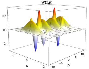
is the Wigner function corresponding to the ground state of the oscillator. The plot of $W(x,p,t)$ for $t=2\pi N$, $\rho=0,\rho=1$ and $\rho=\tau=1/\sqrt{2}$ at $|\mathrm{z}_{+}|=3$ and $|\mathrm{z}_{-}|=9$ is presented in Figs. 4,5.

From Eq. (Evolution of mechanical subsystem and average current),(Evolution of mechanical subsystem and average current) one can see that in the case when $\rho$ is equal to zero or one (in particular, when $t_{s}=0$) the Wigner function is positive and has two maxima, demonstrating the entanglement between two states of the qubit and two coherent states (see Fig. 4). In general case $\rho\tau\neq 0$, and the Wigner function takes both positive and negative values at $t>t_{s}$, demonstrating the entanglement of two states of the qubit with two states of the nanomechanical resonator (see Fig. 5).

As it follows from the above consideration, the amplitude of mechanical fluctuations, and therefore the energy stored in the mechanical subsystem, changes over time. This energy comes from the electronic subsystem causing a rectification of ac current. To analyze this phenomenon, we calculate the dimensionless (normalized to $I_{0}=2e/\hbar$) ac Josephson current averaged over the N-th period of the Josephson oscillations:

$$I_{N}=\frac{1}{2\pi}\int\limits^{2\pi N}_{2\pi(N-1)}dt\mathrm{Tr}\left(\frac{\partial\hat{H}_{q}(t)}{\partial\Phi}\hat{\varrho}(t)\right).$$

Taking into account that $\partial\hat{H}_{q}/\partial\Phi=\eta\partial\hat{H}/\partial t$ and $\hat{H}_{q}(t=2\pi N)=0$, one gets the following expression for $I_{N}$,

	$\displaystyle I_{N}=\frac{\eta}{2\pi}\nabla_{N}\mathrm{Tr}\left(\hat{H}_{m}+\hat{H}_{int}\right)\hat{\varrho}(2\pi N)$
	$\displaystyle\hskip 17.07182pt=\frac{\eta}{2\pi}\nabla_{N}\left[E_{m}(N)+E_{int}(N)\right],$		(25)

where $\nabla_{N}f(N)\equiv f(N)-f(N-1)$ is the first difference. From this equation, one can see that the average current is given by the change of the mechanical energy $E_{m}$ and the energy of interaction $E_{int}$ after N-th period. One can find that at $N>Ns=[t_{s}/2\pi]+1$ the functions $E_{m}(N)$ and $E_{int}(N)$ can be written as follows,

	$\displaystyle E_{m}(N)=2\pi^{2}\tilde{\varepsilon}^{2}\left(\rho^{2}(2N_{s}-N)^{2}+\tau^{2}N^{2}\right),$
	$\displaystyle E_{int}(N)=2\pi\varepsilon\tilde{\varepsilon}\left[\rho^{2}\left(N-2N_{s}\right)\text{e}^{-(2\pi\tilde{\varepsilon})^{2}(N-2N_{s})^{2}}+\right.$
	$\displaystyle\hskip 36.98866pt\left.+\tau^{2}N\text{e}^{-(2\pi\tilde{\varepsilon}N)^{2}}\right].$		(26)

The change in the interaction energy contributes to the averaged current as well as the mechanical energy. However, this contribution is of the order of $\tilde{\varepsilon}^{2}$ and important only for periods for which $I(N)/\tilde{\varepsilon}\simeq\tilde{\varepsilon}^{2}$. So, the average current is determined by the change of mechanical energy mainly, and is defined by the following equations,

	$\displaystyle\frac{I(N)}{\tilde{\varepsilon}}\approx I_{m}(N)=-2\pi\tilde{\varepsilon}N,\hskip 14.22636ptN\leq N_{s}-1$		(27)
	$\displaystyle\frac{I(N)}{\tilde{\varepsilon}}\approx 2\pi\tilde{\varepsilon}\left(N-2\rho^{2}N_{s}\right),\hskip 14.22636ptN>N_{s}.$		(28)

From Fig. 6 one can see that the averaged current exhibits a jump equal to $-\rho^{2}I(N_{s})$ after the period during which the bias voltage is switched. It originates in the fact that when we switch the sign of the bias voltage (at $t=t_{s}$) the power, pumped into the mechanical subsystem, changes depending on the magnitude of $\rho^{2}$. For $\rho=1$, the supplied power, $P=IV$, just changes its sign with the bias voltage, and the current continues to flow in the same direction as it did before switching. For $\rho=0$ supplied power is not changed and consequently the current direction changes after switching.

In conclusion, we have analyzed quantum dynamics of the NEMS comprising the movable CPB qubit, subjected to an electrostatic field and coupled to the two bulk superconductors,controlled by the bias voltage, via tunneling processes. We demonstrate analytically that if the ac Josephson frequency of superconductors, controlled by the bias voltage, is in resonance with the mechanical frequency of the CPB, the initial pure state (direct product of the CPB state and ground state of the oscillator) evolves in time into the coherent states of the mechanical oscillator entangled with the qubit states. Furthermore, we established the protocol of the bias voltage manipulation which results in the formation of entangled states incorporating so-called cat-states (the quantum superposition of the coherent states). The organization of such states is confirmed by the analysis of the corresponding Wigner function taking negative values, while their specific features provide the possibility for their experimental detection by measuring the average current. The discussed phenomena may serve as a foundation for the encoding of quantum information from charge qubits into a superposition of the coherent mechanical states. It may constitute interest for the field of quantum communications due to the robustness of such multiphonon states regarding external perturbation, comparing to the single-phonon Fock state. However, the discussion of the specific protocols for such encoding is out of the scope of this paper and will be presented elsewhere.

The authors thank I.V. Krive and R.I. Shekhter for the useful discussions. This work was partially supported by the Institute for Basic Science in Korea (IBS-R024-D1). LYG thanks the IBS Center for Theoretical Physics of Complex Systems, Daejeon, Rep. of Korea, for their hospitality.

References

- (1) K.L. Ekincia, M.L. Roukes, Review of Scientific Instruments 76, 061101 (2005).
- (2) Y. Nakamura, Yu.A. Pashkin and J.S. Tsai, Nature 398, 786-788 (1999).
- (3) S. Schmid, L.G. Villanueva, and M. Roukes, Fundamentals of Nanomechanical Resonators, Springer, Switzerland (2016).
- (4) K.J. Satzinger, Y.P. Zhong, H-S. Chang, G.A. Peairs, A. Bienfait, M.-H. Chou, A.Y. Cleland, C.R. Conner, E. Dumur, J. Grebel, I. Gutierrez, B.H. November, R.G. Povey, S.J. Whiteley, D.D. Awschalom, D.I. Schuster, A.N. Cleland, Nature 563, 661 (2019).
- (5) A. Bienfait, K.J. Satzinger, Y.P. Zhong, H.-S. Chang, M.-H. Chou, C.R. Conner, E. Dumur, J. Grebel, G.A. Peairs, R.G. Povey, A.N. Cleland, Science Vol.364, Issue 6438, 368 (2019).
- (6) Y. Chu, P. Kharel, W.H. Renninger, L.D. Burkhart, L. Frunzio, P.T. Rakich, R.J. Schoelkopf, Science 358, 6360, Issue 199 (2017).
- (7) M.-H. Chou, E. Dumur, Y.P. Zhong, G.A. Peairs, A. Bienfait, H.-S. Chang, C.R. Conner, J. Grebel, R.G. Povey, K.J. Satzinger and A.N. Cleland, to be published, ArXiv: 2012.04583 [quant-ph]
- (8) M.D. LaHaye, J. Suh, P.M. Echternach, K.C. Schwab and M.L. Roukes, Nature 459, 960 (2009).
- (9) L. Tian, Phys.Rev.B 72, 195411 (2005).
- (10) L.Y. Gorelik, A. Isacsson, Y.M. Galperin, et al., Nature 411, 454 (2001)
- (11) A. Isacsson, L.Y. Gorelik, R.I. Shekhter, Y.M. Galperin, and M. Jonson, Phys.Rev.Lett. 89, 277002 (2002).
- (12) S.M. Girvin, Phys.Rev.Lett. 123, 250501 (2019).
- (13) S.M. Girvin, arXiv:1710.03179v1 [quant-ph] (2017)
- (14) K. Masuda, S. Moriyama, Y. Morita, K. Komatsu, T. Takagi, T. Hashimoto, N. Miki, T. Tanabe, and H. Maki, Appl. Phys. Lett. 108, 222601 (2016).
- (15) A. Bezryadin and P.M. Goldbart, Adv.Mater. 22, 1111-1121 (2010).
- (16) P. Arrangoiz-Arriola, E.A. Wollack, Z. Wang et al. Nature 571, 537 (2019).