Ensembles of Compact, Region-specific & Regularized
Spiking Neural Networks for Scalable Place Recognition
Abstract
Spiking neural networks have significant potential utility in robotics due to their high energy efficiency on specialized hardware, but proof-of-concept implementations have not yet typically achieved competitive performance or capability with conventional approaches. In this paper, we tackle one of the key practical challenges of scalability by introducing a novel modular ensemble network approach, where compact, localized spiking networks each learn and are solely responsible for recognizing places in a local region of the environment only. This modular approach creates a highly scalable system. However, it comes with a high-performance cost where a lack of global regularization at deployment time leads to hyperactive neurons that erroneously respond to places outside their learned region. Our second contribution introduces a regularization approach that detects and removes these problematic hyperactive neurons during the initial environmental learning phase. We evaluate this new scalable modular system on benchmark localization datasets Nordland and Oxford RobotCar, with comparisons to standard techniques NetVLAD, DenseVLAD, and SAD, and a previous spiking neural network system. Our system substantially outperforms the previous SNN system on its small dataset, but also maintains performance on 27 times larger benchmark datasets where the operation of the previous system is computationally infeasible, and performs competitively with the conventional localization systems.
I Introduction
Spiking neural networks (SNNs) closely resemble biological neural networks [1]. Each neuron has an internal state representing its current activation, and information transfer between neurons is sparsely transmitted via spikes that occur when a neuron’s internal activation exceeds a threshold [2]. Spiking networks, when deployed on tailored neuromorphic processors, have the potential to be extremely energy efficient and process data with low latencies [3, 4].

SNNs have thus been used in a number of robotics applications [5, 6, 7, 8, 9, 10, 11, 12], including the visual place recognition (VPR) task [13, 14] that is considered in this paper. A VPR system has to find the matching reference image given a query image of a place, with the difficulty that the appearance of the query image can differ significantly from the reference image due to change in season, time of the day, or weather conditions [15, 16, 17, 18]. VPR is crucial in a range of robot localization tasks, including loop closure detection for Simultaneous Localization and Mapping (SLAM) [15, 16, 17, 18].
Thus far SNNs have not been widely applied in VPR tasks. One key limitation of prior works [14, 13] is the specialization in only small-scale environments. In this work, we aim to increase the capacity of SNNs to an order of magnitude larger environments. We do so by taking inspiration from the brain, which commonly uses a modular organization of neuron groups that act in parallel to efficiently perform complex recognition tasks [19, 20]. Specifically, there is evidence of an ensemble effect for perception and learning tasks [21, 22, 23, 24].
In our work, we implement such an ensemble by deriving SNNs for VPR that take a divide and conquer approach [25]. Each local region of the environment is encoded in a compact, localized SNN, which is responsible only for this local region. At deployment time, all localized encoders compete with each other and are free to respond to any place, resulting in a highly scalable and parallelizable system. This concept is also known as a mixture of experts, where each ensemble member is an expert on a sub-task (in our case a local region of the environment), and all ensemble members cooperate to perform prediction for complex learning tasks (in our case recognizing places in a large-scale environment) [25, 26].
We note that there are other types of ensemble learning that average the prediction of e.g. different classifiers, but within this paper, we refer to ensembles that specialize on distinct subsets of the training data. Such independent processing overcomes the computational constraints that arise when increasing the network size in a non-modular spiking network [27].
While being higly scalable, localized SNNs do not interact with other ensemble members at training time and have no global regularization. As a result, some neurons erroneously respond to places outside their area of expertise. In this work, we refer to these neurons as hyperactive. Our proposed regularization approach improves model performance by detecting and removing these problematic hyperactive neurons.
The key contributions of our work are:
-
1.
We introduce the concept of ensemble spiking neural networks for scalable visual place recognition (Figure 1). Each ensemble member is compact and specializes in a local region of the environment at training time. At deployment time, the query image is provided to all ensemble members in parallel, followed by a fusion of the place predictions.
-
2.
As each ensemble member focuses independently on a local region of the environment, there is a lack of global regularization. After training the ensemble members, we detect hyperactive neurons, i.e. neurons that frequently respond to images outside their training area, and ignore the responses of these hyperactive neurons at deployment time.
-
3.
We demonstrate that our method outperforms prior spiking networks [14] both on small datasets (for which [14] was designed for) and large datasets containing over 2,500 images, where [14] catastrophically fails. Our method performs competitively when compared to conventional VPR methods, namely NetVLAD [28], DenseVLAD [29] and SAD [30], on the Nordland [31] and Oxford RobotCar [32] datasets.
To foster future research, we make our code available: https://github.com/QVPR/VPRSNN.
II Related works
In this section, we review spiking neural networks in robotics research (Section II-A), ensemble neural networks concepts (Section II-B), and key related works on visual place recognition (Section II-C).
II-A Spiking neural networks in robotics research
The neuromorphic computing field develops hardware, sensors and algorithms that are inspired by biological neural networks, with the aim of exploiting their advantages including robustness, generalization capabilities, and incredible energy efficiency [33, 4]. Spiking neural networks are one class of algorithms considered within neuromorphic computing.
Such spiking neural networks can be trained via unsupervised methods such as Spike-Timing-Dependent-Plasticity [34], or by converting pre-trained conventional artificial neural networks to spiking networks [35, 36, 37]. ANN-to-SNN conversion approaches have demonstrated comparable performance to their ANN equivalents; however, these approaches typically cannot fully exploit the advantages of SNNs. We note that the non-differentiable nature of spikes in SNNs prevents direct application of supervised techniques such as back-propagation; however, some recent works proposed solutions to approximate back-propagation for SNNs [38, 39].
Thanks to their desirable characteristics, SNNs have gathered interest in a range of robotics applications, including control [5, 6, 7, 8], manipulation [9, 10], scene understanding [11], and object tracking [12]. Key works that use spiking networks for robot localization, the task considered in this paper, include an energy-efficient uni-dimensional SLAM [40], a robot navigation controller system [41], a pose estimation and mapping system [42], and models of the place, grid and border cells of rat hippocampus [43] based on RatSLAM [44].
However, thus far the performance of these methods have only been demonstrated in simulated [43, 42], constrained indoor [40, 41], or small-scale outdoor environments [14]. The most similar prior work is [14] which introduced a high-performing SNN for VPR. However, [14] was limited to recognizing just 100 places, compared to several thousand places in our proposed ensemble spiking networks.
II-B Ensemble neural networks
Ensemble neural networks contain multiple ensemble members, with each ensemble member being responsible for a simple sub-task [25, 26, 27]. In this paper, we decompose the learning data so that each ensemble member is trained in parallel on a disjoint subset of the data [27].
Various ensemble schemes have been used in SNN research, including unsupervised ensembles for spiking expectation maximization networks [45]. The most similar ensemble SNN is that of [46]. However, each ensemble member in [46] learns a portion of an input image, opposed to different sections of the input data as in our work.
II-C Visual place recognition
Visual place recognition (VPR) is the task of recognizing a previously visited place despite changes in appearance and perceptual aliasing [15, 16]. VPR is often considered as a template matching problem, where the query image is matched to the most similar reference image.
Recent works on VPR are dominated by deep learning. A widely-known deep learning approach is NetVLAD [28], which is based on the Vector of Locally Aggregated Descriptors (VLAD) [47], trained end-to-end thanks to a differentiable pooling layer. Many works extended NetVLAD in several directions [48, 49, 50, 51]. As NetVLAD still performs competitively, we use it for benchmarking in this work.
Bio-inspiration has a long history in VPR research: The hippocampus of rodent brains has inspired RatSLAM [44], 3D grid cells and multilayer head direction cells inspired [52], and cognitive processes of fruit flies inspired [53]. Other works are based on spatio-temporal memory architectures [54, 55]. We note that the detection and removal of hyperactive neurons in our approach is conceptually similar to using salient features of a place representation [56].
III Methodology
The core idea in our method (Figure 1) is to train compact spiking networks that learn a local region of the environment (Section III-A). By combining the predictions of these localized networks at deployment time within an ensemble scheme (Section III-B) and introducing global regularization (Section III-C), we enable large-scale place recognition.
III-A Preliminaries
Our ensemble is homogeneous, i.e. each expert within the ensemble has the same architecture and uses the same hyperparameters. The experts only differ in their training data, which consists of geographically non-overlapping regions of the environment. The training of a single expert spiking network follows [57, 14] and is briefly introduced for completeness in this subsection.
Network structure: Each expert module consists of three layers: 1) The input layer transforms each input image into Poisson-distributed spike trains via pixel-wise rate coding. The number of input neurons corresponds to the number of pixels in the input image: , where and correspond to the width and height of the input image respectively. 2) The input neurons are fully connected to excitatory neurons. Each excitatory neuron learns to represent a particular stimulus (place), and a high firing rate of an excitatory neuron indicates high similarity between the learned and presented stimuli. Note that multiple excitatory neurons can learn the same place. 3) Each excitatory neuron connects to exactly one inhibitory neuron. These inhibitory neurons inhibit all excitatory neurons except the excitatory neuron it receives a connection from. This enables lateral inhibition, resulting in a winner-takes-all system.
Neuronal dynamics: The neuronal dynamics of all neurons are implemented using the Leaky-Integrate-and-Fire (LIF) model [2], which describes the internal voltage of a spiking neuron in the following form:
| (1) |
where is neuron time constant, is the membrane potential at rest, and are the equilibrium potentials of the excitatory and inhibitory synapses with synaptic conductance and respectively.
Network connections: The connections between the inhibitory and excitatory neurons are defined with constant synaptic weights. The synaptic conductance between input neurons and excitatory neurons is exponentially decaying, as modeled by:
| (2) |
where the time constant of the excitatory postsynaptic neuron is . The same model is used for inhibitory synaptic conductance with the inhibitory postsynaptic potential time constant .
Weight updates: The biologically inspired unsupervised learning mechanism Spike-Timing-Dependent-Plasticity (STDP) is used to learn the connection weights between the input layer and excitatory neurons. Connection weights are increased if the presynaptic spike occurs before a postsynaptic spike, and decreased otherwise. The synaptic weight change after receiving a postsynaptic spike is defined by:
| (3) |
where is the learning rate, records the number of presynaptic spikes, is the presynaptic trace target value when a postsynaptic spike arrives, is the maximum weight, and is a ratio for the dependence of the update on the previous weight.
Local regularization: To prevent individual neurons from dominating the response, homeostasis is implemented through an adaptive neuronal threshold. The voltage threshold of the excitatory neurons is increased by a constant after the neuron fires a spike, otherwise the voltage threshold decreases exponentially. We note that the homeostasis provides regularization only on the local, expert-specific scale, not on the global ensemble-level scale.
Neuronal assignment: The network training encourages the network to discern the different patterns (i.e. places) that were presented during training. As the training is unsupervised, one needs to assign each of the excitatory neurons to one of the training places (). Following [57], we record the number of spikes of the -th excitatory neuron when presented with an image of the -th place. The highest average response of the neurons to place labels across the local training data is then used for the assignment , such that neuron is assigned to place if:
| (4) |
Place matching decisions: Following [57], given a query image , the matched place is the place which is the label assigned to the group of neurons with the highest sum of spikes to the query image . Formally:
| (5) |
III-B Ensemble Scheme
The previous section described how to train individual spiking networks following [14]. In this section, we present our novel ensemble spiking network, which consists of a set of experts. The -th expert is tasked to learn the places contained in non-overlapping subsets of the reference database , whereby
| (6) |
All subsets are of equal size, i.e. . Therefore, at training time the expert modules are independent and do not interact with each other, a key enabler of scalability.
At deployment time, the query image is provided as input to all experts in parallel. The place matching decision is obtained by considering the spike outputs of all ensemble members, rather than just a single expert as in Eq. (5).
III-C Hyperactive neuron detection
The basic fusion approach that considers all spiking neurons of all ensemble members is problematic. As the expert members are only ever exposed to their local subset of the training data, there is a lack of global regularization to unseen training data outside of their local subset. In the case of spiking networks, this phenomenon leads to “hyperactive” neurons that are spuriously activated when stimulated with images from outside their training data. We decided to detect and remove these hyperactive neurons.
To detect hyperactive neurons, we do not require access to query data. We use the cumulative number of spikes fired by neurons of each module in response to the entire reference dataset . indicates the number of spikes fired by neuron of module in response to image . Neuron is considered hyperactive if
| (7) |
where is a threshold value that is determined as described in Section III-D. The place match is then obtained by the highest response of neurons that are assigned to place after ignoring all hyperactive neurons:
| (8) |
where the indicator function filters all hyperactive neurons.
III-D Hyperparameter search
We use a grid search to tune the network’s hyperparameters: the time constant of the inhibitory synaptic conductance , and the threshold value to detect the hyperactive neurons . We train the modules multiple times using the reference images introduced in Section III-B, and vary and . We then observe the performance in response to a query set which is geographically separate from the test set .
Specifically, for each combination of the hyperparameter values, we evaluate the performance of the ensemble SNN model on the calibration images using the precision at 100% recall metric (see Section IV-C). We select the and hyperparameter values that lead to the highest performance and use these values for all test images at deployment time.
IV Experimental Setup
IV-A Implementation details
We implemented our ensemble spiking neural network in Python3 and the Brian2 simulator [58]. We pre-processed all reference and query input images by resizing images to pixels, and patch-normalizing images [30] using patches of size pixels.
We use rate coding to convert input images to Poisson spike trains. The number of neurons in the input layer corresponds to the number of pixels in the input image. We used consecutive places to train each ensemble member. The hyperparameter search in Section III-D resulted in and for the Nordland dataset, and with for the Oxford RobotCar dataset. Given an input image, the number of spikes of the excitatory (output) neurons in the last 10 epochs are recorded. The SNN modules were trained in parallel for 60 epochs irrespective of the dataset.
IV-B Datasets
We evaluated our ensemble spiking neural network on two widely used VPR datasets, Nordland [31] and Oxford RobotCar [32]. The Nordland dataset [31] captures a 728 km train journey in Norway where the same traverse is recorded during spring, summer, fall and winter. As in prior works [59, 60, 49] tunnels and sections where the train travels below 15 km/hr were removed. We trained our model on the spring and fall traverses, and we used summer traverse as the query dataset. We subsampled places every 8 seconds (about 100 meters) from the entire dataset, resulting in 3300 places. The Oxford RobotCar dataset [32] contains over 100 traversals captured under varying weather conditions, times of the day and seasons. As in [59], our reference dataset consists of sun (2015-08-12-15-04-18) and rain (2015-10-29-12-18-17) traverses, and our query dataset is the dusk (2014-11-21-16-07-03) traverse. We sampled places roughly every 8 seconds (about 100 meters), resulting in 450 places.
IV-C Evaluation metrics
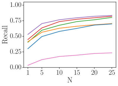
The precision at 100% recall (P@100R) is the percentage of correct matches when the system is forced to match each query image to one of the reference images. The recall at (R@N) metric is the percentage of correct matches if at least one of the top predicted place labels is correctly matched.
We consider a query image to be correctly matched only if it is matched exactly to the correct place – our ground truth tolerance is zero, noting that the distance between the sampled places within the datasets is relatively small.
IV-D Baseline methods
We compare the performance of our method against three conventional VPR approaches: Firstly, the Sum-of-Absolute-Differences (SAD) [30] which computes the pixel-wise difference between each query image and all reference images. For a fair comparison, we applied the same resizing and patch-normalizing steps as in our approach (see Section IV-A). Secondly, DenseVLAD [29] which uses densely sampled SIFT image descriptors. Lastly, NetVLAD [28] which generalizes across different datasets and is robust to viewpoint and appearance changes. For NetVLAD and DenseVLAD, we used the original input image size of pixels for Nordland and resized the input images to pixels for Oxford RobotCar, potentially giving them an advantage over the low-dimensional input images in our proposed method.
We also compare against a non-ensemble SNN [14], which in [14] was limited to just 100 places because of a relatively small network size. To compare against [14] on our large datasets, we increase the network size of their approach to contain output neurons (i.e. one output neuron per place). We note that increasing the number of neurons in their SNN results in significantly longer training and inference times (Figure 3), so we trained their network for only 26 epochs. In Section V-C, we additionally compare our method to [14] in a small-scale environment (for which [14] was designed).
V Results
In this section, we first provide a performance comparison of our ensemble SNN model against NetVLAD [28], DenseVLAD [29], Sum-of-Absolute-Differences (SAD) [30] and the currently best performing SNN [14] (Section V-A). We then evaluate the effect of removing hyperactive neurons in Section V-B. Finally, Section V-C provides an ablation study where we demonstrate that in small-scale environments which [14] was designed for, the performance of our ensemble SNN compares to prior non-ensemble SNN [14].
![[Uncaptioned image]](https://cdn.awesomepapers.org/papers/cef93717-fbd7-43a9-b8fb-10639255b1ad/x2.png)


V-A Comparison to state-of-the-art approaches
We first compare our ensemble SNN to conventional VPR techniques, with the aim of merely demonstrating the potential of SNN-based approaches, as opposed to outperforming these VPR techniques. The results are summarized in Table I.
For the Nordland dataset, our ensemble SNN model obtains a R@1 of 52.6%, outperforming SAD (R@1: 45.1%), NetVLAD (R@1: 35.1%) and DenseVLAD (R@1: 37.9%). We note that NetVLAD is known to perform relatively poorly on the rural Nordland dataset, as it was trained on urban data. For the Oxford RobotCar dataset, the R@1 of our ensemble SNN model is 40.5%, while the SAD approach has a similar R@1 of 41.3%, the NetVLAD and DenseVLAD methods obtain a higher R@1 of 44.8% and 53.1% respectively. The performance of our ensemble SNN achieves a similar R@25 to NetVLAD and DenseVLAD, demonstrating the performance capability of our method.
Table I also presents the performance of the previous non-ensemble SNN model [14], which is our main competitor. [14] catastrophically failed to perform place recognition at large-scale, with a precision at 100% recall of just 0.3% on the Nordland and 4.0% on the Oxford RobotCar datasets. We note that [14] specialized in place recognition on small datasets. In addition to poor performance, the large number of output neurons within a single network for [14] results in significantly increased inference times. This is opposed to our modular approach, where the neuronal dynamics of independent and compact ensemble members are cheaper to compute. We highlight the computational advantages and better scalability of our method in Figure 3. The inference times of our method is still slower compared to conventional VPR methods such as NetVLAD. However, deploying our method on neuromorphic hardware can significantly decrease the inference times via use of hardware parallelism.
V-B Importance of hyperactivity detection
This section evaluates that it is crucial to introduce global regularization by detecting and ignoring hyperactive neurons. As shown in Table I and Figure 2b, our ensemble SNN model where hyperactive neurons are ignored improves the precision at 100% recall compared to the base ensemble SNN model (that includes hyperactive neurons) on both Nordland (absolute increase of 16.9%) and Oxford RobotCar (absolute increase of 10.4%). Figure 4 compares the neuron precision of hyperactive and non-hyperactive neurons trained on the Nordland dataset and highlights that the precision at recognizing correct places of non-hyperactive neurons is significantly higher than that of hyperactive neurons.
We further evaluate the sensitivity of our ensemble SNN with respect to the threshold value (see Section III-D). Specifically, we evaluate the precision at 100% recall at different threshold values (). Note that corresponds to the baseline performance where both hyperactive and non-hyperactive neurons are used. For both the Nordland and Oxford RobotCar datasets, Figure 5 shows that our method is not sensitive to particular values of , with a wide range of high-performing settings. Importantly, any improves performance compared to the baseline model where hyperactive neurons are included ().


V-C Comparison to prior SNN in small environments
This ablation presents a like-for-like comparison of our proposed ensemble SNN and a non-ensemble SNN model from [14] which facilitates direct comparison to the previous state-of-the-art VPR system using SNNs. As [14] was designed for small-scale datasets, we do so by considering a much smaller dataset limited to 100 places; the previous section has already shown that [14] fails catastrophically in large environments. Specifically, we trained ensemble members, each containing excitatory neurons. We used the first places to calibrate and .
The P@100R of our proposed ensemble SNN model at 91.0% is considerably higher than that of prior work on non-ensemble SNNs [14] (79.0%), which in conjunction with the results in Section V-A demonstrates that our ensemble method is both scalable and provides improved performance in both small and large scale environments. The PR curve for these experiments is shown in Figure 6.

VI Conclusions and Future Work
In this paper, we demonstrated that an ensemble of spiking neural networks can perform the visual place recognition task massively parallelized. Each ensemble member specializes in recognizing a small subset of places within a local region. Typically local ensemble members operate independently without any global regularization. We introduce global regularization by detecting and ignoring hyperactive neurons, which respond strongly to previously unseen places. Our experiments demonstrated significant performance gains and scalability improvements compared to prior SNNs, and comparable performance to NetVLAD, DenseVLAD and SAD.
Future work will follow a number of research directions. We will investigate how our approach can be made robust to significant viewpoint changes. We are investigating to use event streams (from event cameras) as input data, instead of converting images to spike trains via rate coding, to further reduce the power requirements and localization latency. We are working towards implementing our method on Intel’s neuromorphic processor, Intel Loihi [4]. Deployment on neuromorphic hardware in similar applications [3] has demonstrated high energy efficiency, high throughput and low latency. Finally, we will investigate integrating our VPR system into a full SNN-based SLAM pipeline.
References
- [1] S. Ghosh-Dastidar and H. Adeli, “Spiking neural networks,” Int. J. Neural Syst., vol. 19, no. 04, pp. 295–308, 2009.
- [2] W. Gerstner, W. M. Kistler, R. Naud, and L. Paninski, Neuronal dynamics: From single neurons to networks and models of cognition. Cambridge University Press, 2014.
- [3] E. P. Frady et al., “Neuromorphic nearest neighbor search using Intel’s Pohoiki Springs,” in Proc. Neuro-inspired Comput. Elements Worksh., 2020.
- [4] M. Davies et al., “Advancing neuromorphic computing with Loihi: A survey of results and outlook,” Proc. IEEE, vol. 109, no. 5, pp. 911–934, 2021.
- [5] I. Abadía, F. Naveros, E. Ros, R. R. Carrillo, and N. R. Luque, “A cerebellar-based solution to the nondeterministic time delay problem in robotic control,” Science Robotics, vol. 6, no. 58, p. eabf2756, 2021.
- [6] A. Vitale, A. Renner, C. Nauer, D. Scaramuzza, and Y. Sandamirskaya, “Event-driven vision and control for UAVs on a neuromorphic chip,” in IEEE Int. Conf. Robot. Autom., 2021, pp. 103–109.
- [7] J. Dupeyroux, J. J. Hagenaars, F. Paredes-Vallés, and G. C. de Croon, “Neuromorphic control for optic-flow-based landing of mavs using the loihi processor,” in IEEE Int. Conf. Robot. Autom., 2021, pp. 96–102.
- [8] R. K. Stagsted, A. Vitale, A. Renner, L. B. Larsen, A. L. Christensen, and Y. Sandamirskaya, “Event-based pid controller fully realized in neuromorphic hardware: a one dof study,” in IEEE/RSJ Int. Conf. Intell. Robot. Syst., 2020, pp. 10 939–10 944.
- [9] J. C. V. Tieck et al., “Towards grasping with spiking neural networks for anthropomorphic robot hands,” in Int. Conf. Artificial Neural Netw., 2017, pp. 43–51.
- [10] J. C. V. Tieck, L. Steffen, J. Kaiser, A. Roennau, and R. Dillmann, “Controlling a robot arm for target reaching without planning using spiking neurons,” in IEEE Int. Conf. Cogn. Informatics Cogn. Comput., 2018, pp. 111–116.
- [11] R. Kreiser et al., “An on-chip spiking neural network for estimation of the head pose of the iCub robot,” Front. Neurosci., vol. 14, no. 551, 2020.
- [12] A. Lele, Y. Fang, J. Ting, and A. Raychowdhury, “An end-to-end spiking neural network platform for edge robotics: From event-cameras to central pattern generation,” IEEE Trans. Cogn. Devel. Syst., 2021.
- [13] L. Zhu, M. Mangan, and B. Webb, “Spatio-temporal memory for navigation in a mushroom body model,” in Conf. Biomimetic Biohybrid Syst., 2020, pp. 415–426.
- [14] S. Hussaini, M. Milford, and T. Fischer, “Spiking neural networks for visual place recognition via weighted neuronal assignments,” IEEE Robot. Autom. Lett., vol. 7, no. 2, pp. 4094–4101, 2022.
- [15] S. Garg, T. Fischer, and M. Milford, “Where Is Your Place, Visual Place Recognition?” in Int. Joint Conf. Artif. Intell., 2021, pp. 4416–4425.
- [16] S. Lowry, N. Sünderhauf, P. Newman, J. J. Leonard, D. Cox, P. Corke, and M. J. Milford, “Visual place recognition: A survey,” IEEE Trans. Robot., vol. 32, no. 1, pp. 1–19, 2015.
- [17] C. Masone and B. Caputo, “A survey on deep visual place recognition,” IEEE Access, vol. 9, pp. 19 516–19 547, 2021.
- [18] X. Zhang, L. Wang, and Y. Su, “Visual place recognition: A survey from deep learning perspective,” Pattern Recognition, vol. 113, p. 107760, 2021.
- [19] V. Mountcastle, “An organizing principle for cerebral function: the unit module and the distributed system,” The Mindful Brain, 1978.
- [20] L. Krubitzer, “The organization of neocortex in mammals: are species differences really so different?” Trends in Neurosciences, vol. 18, no. 9, pp. 408–417, 1995.
- [21] F. Varela, J.-P. Lachaux, E. Rodriguez, and J. Martinerie, “The brainweb: phase synchronization and large-scale integration,” Nature Reviews Neuroscience, vol. 2, no. 4, pp. 229–239, 2001.
- [22] R. C. O’Reilly, “Modeling integration and dissociation in brain and cognitive development,” Processes of Change in Brain and Cognitive Development: Attention and Performance, vol. 21, pp. 375–402, 2006.
- [23] A. S. Bock and I. Fine, “Anatomical and functional plasticity in early blind individuals and the mixture of experts architecture,” Front. Human Neurosci., vol. 8, p. 971, 2014.
- [24] W. Li, J. D. Howard, T. B. Parrish, and J. A. Gottfried, “Aversive learning enhances perceptual and cortical discrimination of indiscriminable odor cues,” Science, vol. 319, no. 5871, pp. 1842–1845, 2008.
- [25] R. A. Jacobs, M. I. Jordan, S. J. Nowlan, and G. E. Hinton, “Adaptive mixtures of local experts,” Neural Computation, vol. 3, no. 1, pp. 79–87, 1991.
- [26] B. L. Happel and J. M. Murre, “Design and evolution of modular neural network architectures,” Neural Networks, vol. 7, no. 6-7, pp. 985–1004, 1994.
- [27] G. Auda and M. Kamel, “Modular neural networks: a survey,” International journal of neural systems, vol. 9, no. 02, pp. 129–151, 1999.
- [28] R. Arandjelovic, P. Gronat, A. Torii, T. Pajdla, and J. Sivic, “NetVLAD: CNN architecture for weakly supervised place recognition,” IEEE Trans. Pattern Anal. Mach. Intell., vol. 40, no. 6, pp. 1437–1451, 2018.
- [29] A. Torii, R. Arandjelovic, J. Sivic, M. Okutomi, and T. Pajdla, “24/7 place recognition by view synthesis,” in IEEE Conf. Comput. Vis. Pattern Recog., 2015, pp. 1808–1817.
- [30] M. J. Milford and G. F. Wyeth, “SeqSLAM: Visual route-based navigation for sunny summer days and stormy winter nights,” in IEEE Int. Conf. Robot. Autom., 2012, pp. 1643–1649.
- [31] N. Sünderhauf, P. Neubert, and P. Protzel, “Are we there yet? Challenging SeqSLAM on a 3000 km journey across all four seasons,” in IEEE Int. Conf. Robot. Autom. Worksh., 2013.
- [32] W. Maddern, G. Pascoe, C. Linegar, and P. Newman, “1 year, 1000 km: The Oxford RobotCar dataset,” Int. J. Robot. Res., vol. 36, no. 1, pp. 3–15, 2017.
- [33] Y. Sandamirskaya, M. Kaboli, J. Conradt, and T. Celikel, “Neuromorphic computing hardware and neural architectures for robotics,” Science Robotics, vol. 7, no. 67, p. eabl8419, 2022.
- [34] D. E. Feldman, “The spike-timing dependence of plasticity,” Neuron, vol. 75, no. 4, pp. 556–571, 2012.
- [35] J. Ding, Z. Yu, Y. Tian, and T. Huang, “Optimal ANN-SNN conversion for fast and accurate inference in deep spiking neural networks,” in Int. Joint Conf. Artif. Intell., 2021.
- [36] B. Rueckauer, I.-A. Lungu, Y. Hu, M. Pfeiffer, and S.-C. Liu, “Conversion of continuous-valued deep networks to efficient event-driven networks for image classification,” Front. Neurosci., vol. 11, p. 682, 2017.
- [37] T. Bu, W. Fang, J. Ding, P. Dai, Z. Yu, and T. Huang, “Optimal ann-snn conversion for high-accuracy and ultra-low-latency spiking neural networks,” in Int. Conf. Learn. Represent., 2021.
- [38] A. Renner, F. Sheldon, A. Zlotnik, L. Tao, and A. Sornborger, “The backpropagation algorithm implemented on spiking neuromorphic hardware,” arXiv:2106.07030, 2021.
- [39] C. Lee, S. S. Sarwar, P. Panda, G. Srinivasan, and K. Roy, “Enabling spike-based backpropagation for training deep neural network architectures,” Front. Neurosci., vol. 14, no. 119, pp. 1–22, 2020.
- [40] G. Tang, A. Shah, and K. P. Michmizos, “Spiking neural network on neuromorphic hardware for energy-efficient unidimensional SLAM,” in IEEE/RSJ Int. Conf. Intell. Robot. Syst., 2019, pp. 4176–4181.
- [41] G. Tang and K. P. Michmizos, “Gridbot: an autonomous robot controlled by a spiking neural network mimicking the brain’s navigational system,” in Int. Conf. Neuromorphic Syst., 2018.
- [42] R. Kreiser, A. Renner, Y. Sandamirskaya, and P. Pienroj, “Pose estimation and map formation with spiking neural networks: towards neuromorphic SLAM,” in IEEE/RSJ Int. Conf. Intell. Robot. Syst., 2018, pp. 2159–2166.
- [43] F. Galluppi et al., “Live demo: Spiking RatSLAM: Rat hippocampus cells in spiking neural hardware,” in IEEE Conf. Biomed. Circuits Syst., 2012, p. 91.
- [44] M. J. Milford, G. F. Wyeth, and D. Prasser, “RatSLAM: a hippocampal model for simultaneous localization and mapping,” in IEEE Int. Conf. Robot. Autom., 2004, pp. 403–408.
- [45] Y. Shim, A. Philippides, K. Staras, and P. Husbands, “Unsupervised learning in an ensemble of spiking neural networks mediated by ITDP,” PLoS Computational Biology, vol. 12, no. 10, p. e1005137, 2016.
- [46] P. Panda, G. Srinivasan, and K. Roy, “EnsembleSNN: Distributed assistive STDP learning for energy-efficient recognition in spiking neural networks,” in Int. Joint Conf. Neural Networks, 2017, pp. 2629–2635.
- [47] H. Jégou, M. Douze, C. Schmid, and P. Pérez, “Aggregating local descriptors into a compact image representation,” in IEEE Conf. Comput. Vis. Pattern Recog., 2010, pp. 3304–3311.
- [48] J. Yu, C. Zhu, J. Zhang, Q. Huang, and D. Tao, “Spatial pyramid-enhanced netvlad with weighted triplet loss for place recognition,” IEEE Trans. Neural Netw. Learn. Syst., vol. 31, no. 2, pp. 661–674, 2019.
- [49] S. Hausler, S. Garg, M. Xu, M. Milford, and T. Fischer, “Patch-NetVLAD: Multi-scale fusion of locally-global descriptors for place recognition,” in IEEE Conf. Comput. Vis. Pattern Recog., 2021, pp. 14 141–14 152.
- [50] A. Khaliq, M. Milford, and S. Garg, “MultiRes-NetVLAD: Augmenting place recognition training with low-resolution imagery,” IEEE Robot. Autom. Lett., vol. 7, no. 2, pp. 3882–3889, 2022.
- [51] Y. Xu, J. Huang, J. Wang, Y. Wang, H. Qin, and K. Nan, “ESA-VLAD: A lightweight network based on second-order attention and NetVLAD for loop closure detection,” IEEE Robot. Autom. Lett., vol. 6, no. 4, pp. 6545–6552, 2021.
- [52] F. Yu, J. Shang, Y. Hu, and M. Milford, “NeuroSLAM: A brain-inspired slam system for 3d environments,” Biological Cybernetics, vol. 113, no. 5, pp. 515–545, 2019.
- [53] M. Chancán, L. Hernandez-Nunez, A. Narendra, A. B. Barron, and M. Milford, “A hybrid compact neural architecture for visual place recognition,” IEEE Robot. Autom. Lett., vol. 5, no. 2, pp. 993–1000, 2020.
- [54] V. A. Nguyen, J. A. Starzyk, and W.-B. Goh, “A spatio-temporal long-term memory approach for visual place recognition in mobile robotic navigation,” Robotics and Autonomous Systems, vol. 61, no. 12, pp. 1744–1758, 2013.
- [55] P. Neubert, S. Schubert, and P. Protzel, “A neurologically inspired sequence processing model for mobile robot place recognition,” IEEE Robot. Autom. Lett., vol. 4, no. 4, pp. 3200–3207, 2019.
- [56] P. Newman and K. Ho, “SLAM-loop closing with visually salient features,” in IEEE Int. Conf. Robot. Autom., 2005, pp. 635–642.
- [57] P. U. Diehl and M. Cook, “Unsupervised learning of digit recognition using spike-timing-dependent plasticity,” Front. Comput. Neurosci., vol. 9, no. 99, pp. 1–9, 2015.
- [58] M. Stimberg, R. Brette, and D. F. Goodman, “Brian 2, an intuitive and efficient neural simulator,” Elife, vol. 8, p. e47314, 2019.
- [59] T. L. Molloy, T. Fischer, M. Milford, and G. N. Nair, “Intelligent reference curation for visual place recognition via Bayesian selective fusion,” IEEE Robot. Autom. Lett., vol. 6, no. 2, pp. 588–595, 2020.
- [60] S. Hausler, A. Jacobson, and M. Milford, “Multi-process fusion: Visual place recognition using multiple image processing methods,” IEEE Robot. Autom. Lett., vol. 4, no. 2, pp. 1924–1931, 2019.