Ensemble Monte Carlo Calculations with Five Novel Moves
Abstract
We introduce five novel types of Monte Carlo (MC) moves that brings the number of moves of ensemble MC calculations from three to eight. So far such calculations have relied on affine invariant stretch moves that were originally introduced by Christen (2007), walk moves by Goodman and Weare (2010) and quadratic moves by Militzer (2023). Ensemble MC methods have been very popular because they harness information about the fitness landscape from a population of walkers rather than relying on expert knowledge. Here we modified the affine method and employed a simplex of points to set the stretch direction. We adopt the simplex concept to quadratic moves. We also generalize quadratic moves to arbitrary order. Finally, we introduce directed moves that employ the values of the probability density while all other types of moves rely solely on the location of the walkers. We apply all algorithms to the Rosenbrock density in 2 and 20 dimensions and to the ring potential in 12 and 24 dimensions. We evaluate their efficiency by comparing error bars, autocorrelation time, travel time, and the level of cohesion that measures whether any walkers were left behind. Our code is open source.
1 Introduction
Since the seminal paper by Metropolis et al. (1953), Monte Carlo (MC) techniques, in particular Markov Chain Monte Carlo (MCMC) methods, have been employed in many areas of science including physics, astronomy, geoscience and chemistry (Kalos & Whitlock, 1986; Ferrario et al., 2006; Landau & Binder, 2021). These methods are particularly effective when states in a high-dimensional space need to be studied but only a small but nontrivial subset of the available states are relevant. The distribution of gas molecules in a three-dimensional room is one example to illustrate their effectiveness. A MC simulation would only generate configurations in the dimensional space in which the molecules are more or less evenly distributed in the room, as one would expect. Formally with analytical statistical methods, one would be required to also integrate over highly unlikely configuration, in which, e.g., many molecules are concentrated in one corner of the room. Such states are irrelevant because they only occupy a negligible measure of the accessible configuration space. MC methods are very good in avoiding unlikely configuration and in sampling only a representative subset of the relevant configurations, which makes such MC method orders of magnitude more efficient than exhaustive integration methods. Consequently, MC methods offer no direct access to the entropy nor to free energies but these quantities can be derived indirectly via thermodynamic integration (de Wijs et al., 1998; Wilson & Militzer, 2010, 2012; Wahl et al., 2013; Gonzalez-Cataldo et al., 2014).
In the field of statistical physics, MC methods have thus found numerous applications to sample the states of classical and quantum systems (Binder et al., 2012; Ceperley & Mitas, 1995; Militzer & Pollock, 2002; Driver & Militzer, 2015) that are weighted by the Boltzmann factor,
| (1) |
is the unnormalized probability density of states, , with an energy, . The product of temperature, , and Boltzmann constant, , controls the relative weights of high- and low-energy states. Throughout this article, represents a vector in the dimensional space of states that is to be sampled. We often refer to such vectors as walkers. refers to the th walker in an ensemble while when we discuss the specific sampling functions like the Rosenbrock density or the ring potential, represents the th component of a vector . It should be noted that a walker does not play the role of a particle in physics-based MCMC calculations where typically particles move in 3D space, which leads to a dimensional sampling space. In such applications, one typically moves one or a handful of particles with specialized types of moves that are particularly efficient for specific interactions. The MCMC methods that we discuss in this article are not focused on sampling particle coordinates but are more general. They should for example allow one to construct ensembles of models of Jupiter’s interior for which a walker may represent the masses and composition of certain layers Militzer & Hubbard (2024). So we do not assume that the dimensional sampling space can be divide into equivalent 3D subspaces. When one moves a particle in physics-based simulations, only its 3 coordinates change while when we move a walker here, all its elements are affected.
Besides statistical physics, there is another broad area of applications where MCMC are typically employed. In fields like astrophysis, one often constructs models to match sets of telescope observations or spacecraft measurements (Hubbard et al., 2002; Bolton et al., 2017), , that come with a statistical uncertainty, . MCMC calculations are then used to map out the space of model parameters, , that is compatible with the observations by sampling probability density (Militzer et al., 2019; Movshovitz et al., 2020; Militzer et al., 2022),
| (2) |
The affine invariant MCMC method by Christen (2007) and Goodman & Weare (2010) along with its practical implementation by Foreman-Mackey et al. (2013) have been very popular to solve such kind of sampling problems. Many applications came from the field of astrophysics. For example, the affine sampling method has been employed to detect stellar companions in radial velocity catalogues (Price-Whelan et al., 2018), to study the relationship between dust disks and their host stars (Andrews et al., 2013), to examine the first observations of the Gemini Planet Imager (Macintosh et al., 2014), to analyze photometry data of Kepler’s K2 phase (Vanderburg & Johnson, 2014), to study the mass distribution in our Milky Way galaxy (McMillan, 2017), to identify satellites of the Magellanic Clouds (Koposov et al., 2015), to analyze gravitational-wave observations of a binary neutron star merger (De et al., 2018), to constrain Hubble constant with data of the cosmic microwave background (Bernal et al., 2016), or to characterize the properties of M-dwarf stars (Mann et al., 2015) to name a few applications. On the other hand, Huijser et al. (2022) demonstrated that the affine (linear) stretch moves exhibit undesirable properties when the Rosenbrock density in more than 50 dimensions is sampled.
The MCMC in this article are not taylored towards any specific application nor do they require knowledge of any derivitatives of the sampling function because they may very difficult to compute for complex applications. This means however that the algorithm has little information to distinguish favorable direction to move into from unfavorable ones, and this is why one employs an ensemble of walkers.
Ensemble MC methods propagates an entire ensemble of walkers rather than moving just a single one. While this seems to imply more work, such methods often win out because they harness information from the distribution of walkers in the ensemble to propose favorable moves that have an increased chance of being accepted without the need for a detailed investigation of the local fitness landscape as the traditional Metropolis-Hastings MC method requires. Many extensions of the Metropolis-Hastings approach have been advanced (Andrieu & Thoms, 2008). For example, Haario et al. (2001) use the entire accumulated history along the Monte Carlo chain of states to adjust the shape of the Gaussian proposal function.
Ensembles of walkers are employed in various types of Monte Carlo methods that have been designed for specific applications. In the fields of condensed matter physics and quantum chemistry, ensembles of walkers are employed in variational Monte Carlo (VMC) calculations (Martin et al., 2016) that optimize certain wavefunction parameters with the goal of minimizing the average energy or its variance (Foulkes et al., 2001). Ensembles are used to vectorize or parallelize the VMC calculations. They are also employed generate the initial set of configurations for the walkers in diffusion Monte Carlo (DMC) simulations. In DMC calculations, one samples the groundstate wave function by combining diffusive moves with birth and death processes. An ensemble of walkers is needed to estimate the average local energy so that the birth and death rates lead to a stable population size. Walkers with a low energy are favored and thus more likely to be selected to spawn additional walkers. Walkers in areas of high energy are likely to die out.
The birth and death concepts in DMC have a number of features in common with genetic algorithms that employ a population of individuals (similar to an ensemble of walkers). The best individuals are selected and modified with a variety of approaches to generate the next generation of individuals (Schwefel, 1981; Militzer et al., 1998). The population is needed to establish a fitness scale that enables one to make informed decisions which individuals should be selected for procreation. This scale will change over time as the population migrates towards for favorable regions in the parameter space. This also occurs in DMC calculations as the walker population migrates towards regions of low energy, the average energy in the population stabilizes, and the local energy approaches the ground state energy of the system.
Ensembles of individuals/walkers are not only employed in genetic algorithm but are used in many different stochastic optimization techniques. These methods have primarily been designed for the goal of finding the best state in a complex fitness landscape, or a state that is very close to it, rather than sampling a well-defined statistical distribution function as Monte Carlo method do. Therefore these optimization are much more flexible than Monte Carlo algorithms that typically need to satisfy the detailed balance relation for every move (Kalos & Whitlock, 1986).
The particle swarm optimization method (Kennedy & Eberhart, 1997; J. Kennedy & Eberhart, 2001) employs an ensemble (or swarm) of walkers and successively updates their locations according to a set of velocities. The velocities are updated stochastically using an inertial term and drift terms favor migration towards the best individual in the population and/or towards the global best ever generated.
In general, efficient Monte Carlo methods are required to have two properties. 1) They need to migrate efficiently in parameter space towards the most favorable region. The migration (or convergence) rate is typically measured in Monte Carlo time (or steps). 2) Once the favorable region has been reached and average properties among walkers have stabilized, the Monte Carlo method needs to efficient sample the relevant parameter space. The efficiency of the algorithm is typically measured in terms of the autocorrelation time or the size of the error bars.
Militzer (2023a) recently introduced quadratic MC (QMC) moves and demonstrated that they are more efficient in sampling challenging, curved fitness landscapes than linear stretch moves. Militzer (2023a) also modified the walk move method by Goodman & Weare (2010) by adding a scale factor, which enables one to control the step size of the moves and thus enable one to substantially increase the MC efficiency. All these method propagate an ensemble of walkers and harness information from their location about the fitness landscape rather relying on expert knowledge to chose the promising directions for future MC moves. The goal of this article is to add five types of novel MC moves to the portfolio of available ensemble MC moves because so far there are only three: affine stretch moves that were first introduced by Christen (2007), walk moves by Goodman & Weare (2010), and the quadratic moves by Militzer (2023a). Here we also design a method to compare the efficiency of all these moves and then apply it by conducting simulations for the Rosenbrock density in 2 and 20 dimensions and the ring potential in 12 and 24 dimensions. In general, we do not know what types of moves will prove to be most effective when MC methods are applied to a broad range of problems, so having access to a portfolio of MC moves may prove useful in saving computer time and thus energy.
2 Methods
2.1 Review of Affine, Quadratic, and Walk Moves
To move walker from location to , Goodman & Weare (2010) employed the affine invariant moves that were originally introduced by Christen (2007). From the ensemble, one selects one additonal walker, , to set the stretch direction,
| (3) |
To make such moves reversible, the stretch factor, , must be sampled from the interval where is constant parameter that we controls the step size. To sample the stretch factor, , one has a bit of a choice. Goodman & Weare (2010) followed Christen (2007) when they adopted a function, , that satisfies,
| (4) | |||||
| (5) |
The acceptance probability is given by
| (6) |
where the factor with emerges because one performs a one-dimensional move to sample points in a -dimensions space (see derivations in Christen (2007) and Militzer (2023a)).
In Fig. 1, we illustrate the affine as well as the quadratic moves. For a quadratic move, Militzer (2023a) selects two walkers and from the ensemble to move walker from to .
| (7) |
The interpolation weights are chosen from,
| (8) | |||||
| (9) | |||||
| (10) | |||||
| (11) |
where is the typical Lagrange weighting function that guarantees a proper quadratic interpolation so that if ; if ; and if . One sets and to introduce a scale into the parameter space, .
To satisfy the detailed balance condition, , it is key that we sample the parameters and from the same distribution . The acceptance probability then becomes,
| (12) |
Again a factor of is needed because we sample the one-dimensional space but then switch to the -dimensional parameter space, . In appendix of Militzer (2023a), this factor is derived rigorously from the generalized detailed balance equation by Green & Mira (2001).
Goodman & Weare (2010) also introduced walk moves. To move walker from to , one chooses at random a subset of walkers, . The subset size, , is a free parameter that one needs to choose within where is the total number of walkers. Militzer (2023a) followed Goodman & Weare (2010) in computing the average location all walkers in the subset,
| (13) |
but then modifoed their formula for computing the step size, , by introduding a scaling factor :
| (14) |
are univariate standard normal random numbers. By setting , one obtains the original walk moves, for which the covariance of the step size, , is the same as the covariance of subset . The introdcution of the scaling parameter, , enabled Militzer (2023a) to make smaller (or larger) steps in situations where the covariance of the instantaneous walker distribution is a not an optimal representation of local structure of the sampling function. It was demonstrated that the scaling factor significantly improves the sampling efficiency of the Rosenbrock function and for the ring potential in high dimensions.
2.2 From Quadratic to Order-N Moves
For a quadratic MC move one selects two guide points to move walker from to the new location . The new location is generated by quadratic interpolation in parameter space . Here we now generalize this concept to arbitrary order, . At random, we first select guide points from the ensemble of walkers. Together with the moving walker, we now have points to perform a Lagrange interpolation of order to derive a new location for the moving walker, ,
| (15) |
The interpolation weights, , are given by
| (16) |
where is an dimensional vector that begins with index 0. are the Lagrange polynomials,
| (17) |
where the modular division in guarantees that index referes to vector element if and to element if is larger. This leads to the usual Lagrange interpolation, , that goes through all points so that if and if . For the quadratic moves in Militzer (2023a), we set and to introduce a scale into the parameter space . The arguments for the original and new locations, and , are both sampled at random.
Militzer (2023a) proposed two alternative methods and sampled them either a uniform distribution from or from a Gaussian function with standard deviation that is centered at . For the acceptance probabilities, we use again Eq. 12. For both sampling functions, the parameter controls the average size of the MC steps in and spaces. While the standard deviation of resulting values is equal to for the Gaussian sampling method, it is equal to only for the linear sampling. So the favorable ranges of tend to be a little larger for linear sampling than for the Gaussian method when the best settings of for both methods are compared for the same application, as we will later see.
When we extend the quadratic moves to higher orders here, we still sample and as before but we need to specify the arguments, , for the remaining interpolation points. For a third order interpolation, a natural choice would be , , and . Following this concept, we distribute the arguments uniformly,
| (18) |
so that and . We study how this MC method performs when we choose the order and combined it with linear and Gaussian sampling and different values of . While we see a dependence on when we compare the performance of this method, the performance of the linear sampling method with the best choice was always comparable to that of the Gaussian sampling method with its best . So for simplicity we combine the results with linear and Gaussian sampling into one dataset when we later compare the performance this method for different orders, .
2.3 Directed Quadratic Moves
None of the moves in Goodman & Weare (2010) or Militzer (2023a) nor any other moves in this article make use of the probability values of the other walkers, , when a new location, , for walker is proposed. Currently only their locations, , are employed. Some valuable information might be harnessed by utilizing that a particular walker, , resides in an unlikely location with a probability value, , that much lower than that of the others. (One may recall that the regula falsi method is more efficient in finding the roots of a function than the bisection method because it makes use of the function value while the bisection method only relies on the sign of the values.)
Here we go back the quadratic moves that relies on the walker, , and two guide points and . We assume their probabilities, , came from an energy function, . The factor may be set to 1. We further assume that we can approximate the energy function by the quadratic function, , whose coefficients are chosen so that it interpolates the three known points, , , and . If is positive, it has a minimum at and we can sample from a Gaussian function,
| (19) |
with the standard deviation, .
For the reverse move, one first needs to consider the probability of sampling from the distribution, . To sample , one constructs a different quadratic function, , that interpolates , , and . This introduces an additional factor into the acceptance ratio,
| (20) |
The approach has one caveat because the interpolation coefficient, , may occasionally become negative during the forward or reverse move, in which case the distribution cannot be properly normalized. When this happens if first try to reorder the elements of the vector . If this is not successful we overwrite with , which leads to a stable MC algorithm. We tested it with with linear and Gaussian sampling, and a series of values, .
2.4 Modified Affine and Simplex Moves
Here we introduce three extensions of the affine and quadratic moves. First for our modified affine moves, we linearly interpolate between walkers and to pick a direction for the stretch move of walker, ,
| (21) |
where is a random number chosen uniformly between 0 and 1. In all other respects, the move proceeds like the original affine move. Illustrations of this and the two following moves are given in Fig. 1.
For our affine simplex moves, we set the direction of the stretch move in yet a different way. As guide points, we select walkers from the ensemble, compute their center of mass, and insert it as into Eq. 21. Finally for our quadratic simplex move, we select two separate sets of walkers at random and compute their respective centers of mass before inserting them as of and into Eq. 7. The move then proceeds like our quadratic moves.
3 Applications
3.1 Ring Potential
We test all our MC methods by applying them to two test problems: the ring potential and Rosenbrock density. The ring potential is defined as,
| (22) |
where is a vector in the dimensions. is the distance from the origin in the - plane. The first term ensures that the potential is small along a ring of constant radius, . The second term keeps the magnitude of all remaining parameters, , small. Increasing the positive integer, , makes the walls of the potential around the ring steeper. For this article, we performed calculations with and 24 dimensions while keeping fixed. The last term breaks axial symmetry. We set to small value of 0.01 so that the potential minimum is approximately located at point while the potential is raised at opposing point . Figure 3 of Militzer (2023a) shows an illustration of this effect. The prefactor of the first term in Eq. 22 is introduced so that the location of potential minimum does not shift much with increasing .
We employ the Boltzmann factor, Eq. 1, to convert the energy of the ring potential into a probability function that we can sample. We set so that the equilibrium distribution is reasonably well confined around point . So when we compute the autocorrelation time and the blocked error bar (Allen & Tildesley, 1987) of the potential energy, we initialized the ensemble of walkers around this point. When we want to determine how long it takes the ensemble of walkers to travel around the ring, we initialize the ensemble near the high-energy point, . We define the travel time to be the number of MC moves that are required for ensemble average of to change sign from negative to positive. Based on such a travel time analysis, Militzer (2023a) concluded that employing between and walkers was a reasonable ensemble size while it took larger ensembles a disproportionally long time to travel around the ring.
The ring potential also allows to define and study the cohesion among an ensemble of walkers, which is relevant because all MC methods in this article perform local moves that rely on information of walkers in the ensemble. This means that if the walkers have split up in a highly dimensional and fragmented fitness landscape, or it were initialized that way, it will be challenging to reunited the walkers later. This will likely to lead to a degradation of performance because a distant walker cannot provide useful guidance for a local move. Therefore, we consider cohesion among the walkers to be a favorable trait of an ensemble MC algorithm.
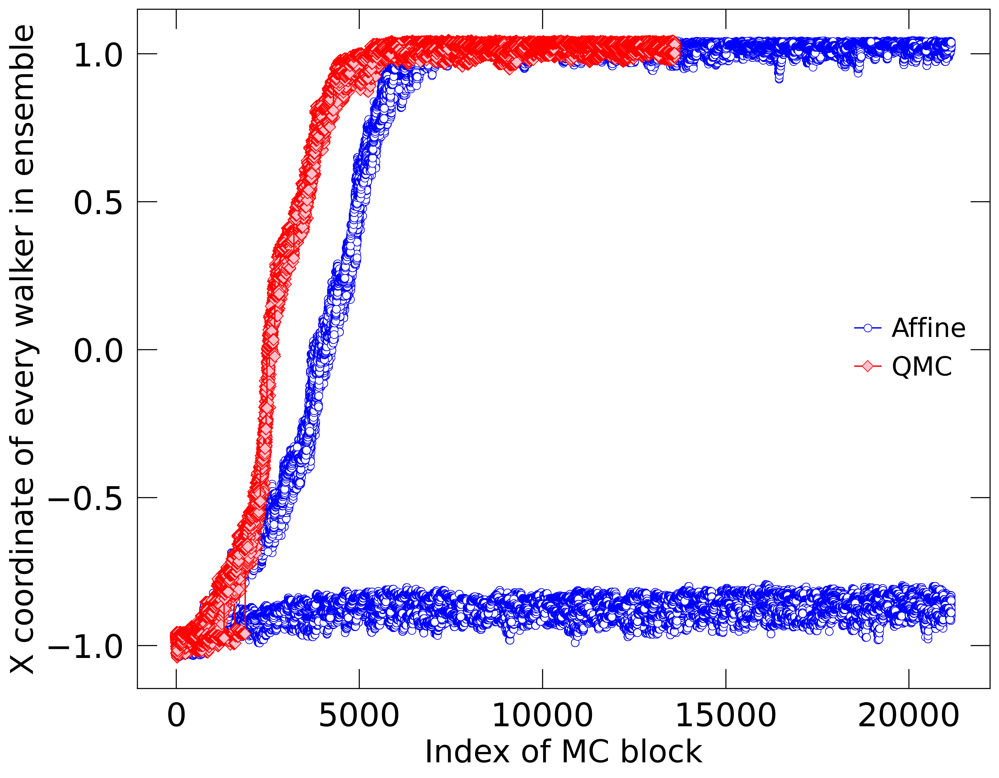
For the ring potential, we define cohesion in the following, simple way. As for the travel time calculation, we initialize the ensemble near the high-energy state of point and then monitor whether all walkers find to their way to the low-energy state near point . Cohesion is defined by the fracton of walkers with at the end of the MC calculation. This average could in principle depend on the duration of the MC calculations but Fig. 2 provides an illustration why this dependence is weak. Conservatively, we end our MC calculations after they completed enough moves equal to twice the ring travel time.
To demonstrate why it is informative to compare the walker cohesion between different MC algorithms, we plot the coordinates of all walkers at the end of every block in Fig. 2. For the ring potential in dimensions, we initialized two ensembles of with walkers near and propagated them with our QMC and with the affine methods. The QMC ensemble remained together and traveled more efficiently towards the low-energy near . The affine ensemble traveled more slowly and split up so that only 17 out of 24 walkers reached the low-energy state. A careful inspection of the first 2000 blocks reveals that even some walkers in the QMC ensemble fell behind but eventually they all caught up. Still one may not expect the QMC ensemble to show perfect cohesion in all circumstances especially if sampling parameters are chose poorly. While Fig. 2 shows just one calculation, we always average the cohesion and the travel time over 1000 independent MC calculations when we compare prediction from different MC moves and parameter settings in this article.
3.2 Rosenbrock Density
Goodman & Weare (2010) tested their methods by sampling the 2d Rosenbrock density,
| (23) |
which carves a narrow curved channel into the landscape. effectively plays the role of temperature while controls the width of the channel. Here we set and to be consistent with Goodman & Weare (2010). There are three different ways one can generalize the Rosenbrock density to higher dimensions. First one can simply treat it as independent 2d Rosenbrock problems by setting,
| (24) |
Alternatively one can “connect” the individual coordinates by defining,
| (25) |
Finally one can make the problem periodic by also connecting the coordinates and ,
| (26) |

In Fig. 3, we compare error bars and autocorrelation times that we computed with all the different MC moves and parameters that we described in Sec. 2 for these three types of Rosenbrock densities in dimensions. We find that the simple Rosenbrock density to be the most challenging one to sample because it leads to the largest error bars and the longest autocorrelation times. Since we are interesting here in designing algorithms that can solve challenging sampling problems, we focus all following investigations on the simple Rosenbrock density and exclude the two others from further consideration. The simple Rosenbrock density was also studied Huijser et al. (2022) who demonstrated that the affine invariant method exhibits undesirable properties in more than 50 dimensions.
4 Results
In this section we compare the efficiency of all types of MC moves for different sampling parameters, one being the size the ensemble, . After Militzer (2023a) demonstrated that setting larger than leads to disproportionally long travel times, we conduct simulations with for all method.
For the affine and the modified affine methods, we conducted simulations with . For the affine simplex method, we combined these four values with using guide points to construct the simplex, which brings the number of separate calculations to 20 for this method.
For the quadratic MC method with linear and Gaussian sampling, we performed simulations for . We use the same set of values to conduct higher-order simulations with , again with both types of sampling. Finally we combined these eight value with guide points to conduct simulations with the quadratic simplex and with the walk method.
This typically led 1224 separate MC calculations for a particular problem and a given dimension. For dimensional Rosenbrock density, this only led to 508 separate MC simulations because in some cases, the number of walkers was too small to allow one to chose the specified number of guide points.
4.1 Rosenbrock results


In Figs. 4 and 5, we respectively compare the results from different MC sampling methods for the Rosenbrock function in and 20 dimensions. In Fig. 6, we show similar results for the ring potential in . We also computed results for dimensions but we do not provide a plot here because they are very similar, with one exception: The order 3 results did not lag behind the QMC results in case as they do for in Fig. 6. One sees the same trend if one compares the and 20 results for the Rosenbrock function.
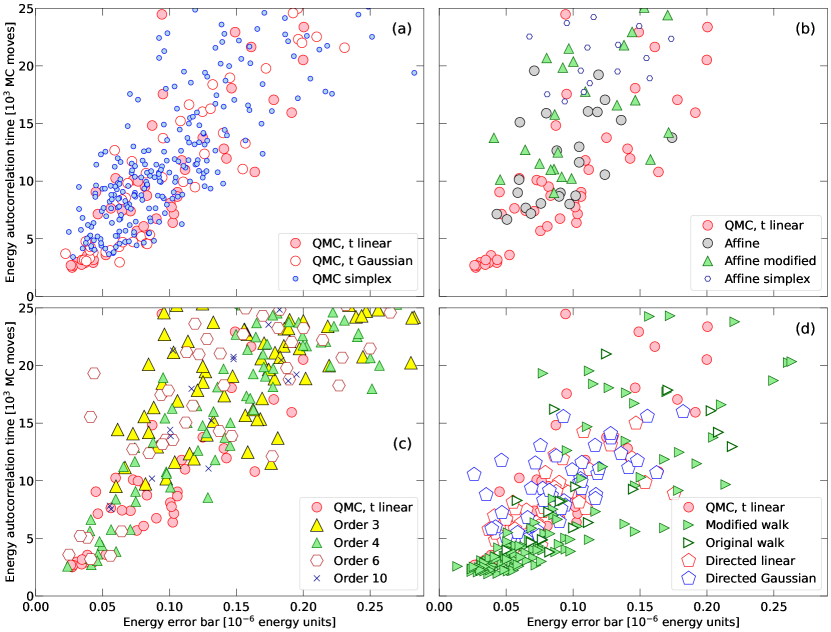
For any application of MC methods, one wants the autocorrelation time and computed averages as small as possible. We compute both for the energy because this is the central quantity of many physical system. The results from different sampling methods are compared in panels (a)-(d) in Figs. 4, 5, and Fig. 6. For the ring potential, an efficient algorithm should fulfill two additional criteria: It should travel efficiently from unfavorable to favorable regions of the parameter space and exhibit a high level of cohesion. Both are plotted in panels (e)-(h) of Fig. 6.
The QMC method with linear and Gaussian sampling yield very good results across all panels in Figs. 4, 5, and 6 but there is also quite a bit of variance among the predictions. So with the following discussion, we identify favorable choice for the different sampling parameters and compare for the two applications with goal of identifying some reasonable default settings for future applications.
For Rosenbrock function in dimensions, the QMC method with linear sampling works well if the scaling parameter is set between 1.0 and 3.0 for any number of walkers between 3 and 7. If is chosen poorly between 0.1 and 0.5, the energy error bar and autocorrelation time increase drastically, which is the trend we see in Fig. 4a. Similarly, the QMC method with Gaussian sampling works well for value between 0.5 and 3.0 and not so well for and 0.3.
If we increase the number of dimensions from 2 to 20, the favorable parameter ranges are slightly modified. The QMC method with linear sampling works well if is set only between 0.3 and 1.0 but not so well for larger values, nor for . The QMC method with Gaussian sampling works well for values between 0.1 and 0.5 but not so well for larger values. As one increases the dimensionality of the Rosenbrock density, sampling the search space becomes more challenging (Huijser et al., 2022) and one needs to make smaller steps to still move efficiently.
When we compare the performance of the QMC method with linear sampling for the ring potential in dimension, we find the method to yield small error bars, short autocorrelation and travel times as well as a high level of cohesion of over 90% if is set between 0.3 and 0.5 for between 26 and 73 walkers.
For , the method works well for between 27 and 49 walkers. If we switch to Gaussian sampling, values between 0.1 and 0.5 yield favorable results. The QMC simplex method yields results that are very similar to that of the original QMC method as Figs. 4, 5, and 6 show consistently. This also means that these test cases did not reveal any particular advantage of this method.
We find that the affine invariant method does not perform as well as the QMC method for all three test cases. It lags behind by factors between 2 and 4 behind the best QMC results as panels (b) of Figs. 4, 5, and 6 show. We obtained the best results for the ring potential by setting and using between 28 and 73 walkers. For these simulations, the cohesion level varied between 80 and 97% (see Fig. 6f). For the Rosenbrock density in 2 and 20 dimensions, we needed to set to 2.5 and 1.2 respectively to obtain the best results. This confirms the trend that sampling the space efficiently requires smaller steps.
Our modification to the affine method did not yield any improvements. In Figs. 5 and 6, it slightly lags behind the original affine method while Figs. 4 shows the autocorrelation time for the 2d Rosenbrock density is about twice as long. The affine simplex performed yet a bit worth. It lagged behind the other affine methods in term of the travel time and cohesion as Fig. 6f shows.
4.2 Ring potential
We obtained the best results for the ring potential in dimensions in Fig. 6 when we employed the QMC method with linear sampling with and Gaussian sampling with . Using between 27 and 73 walkers gave consistently good results. In comparison, the quadratic simplex method did not quite perform as well for any sampling parameters.
Affine and modified affine methods did slightly worse than the quadratic simplex method. The autocorrelation time, error bars, and travel times were not as good and the cohesion varied substantially between 50% and 95% (see Fig. 6b and f). The best choice for the value was 1.2. The affine simplex method performed poorly on all counts.
In Fig. 6c and g, we compare results from interpolations with different orders. Some simulations of fourth and sixth order performed well if we set to 0.1 or 0.3. In comparison, calculations of third and tenth order were not competitive.
In Fig. 6d and h, we compare results obtained with the directed quadratic method and with walk moves. With the directed quadratic method, we obtained the best results by setting to 0.3 and 0.5 but they were not as good as those from original quadratic method. On the other hand, the results from the walk method were consistent better as long as we set the scaling parameter to 0.1 or 0.5, which underlines the importance this parameter that was introduced only recently by Militzer (2023a).
4.3 Relative Inverse Efficiency

The preceeding analysis relied on a detailed comparision of results spread across three figures. So here we introduce the relative inverse efficiency to greatly simplify the comparison of different methods across various applications. Such an efficiency measure should be able to handle the noise that we see in Figs. 4, 5, and 6. Furthermore, one cannot expect that adjustable parameters like and have been optimized to perfection. Instead it should be sufficient to have results for good number of reasonable and values in the dataset. Also a method should not be penalized very much if in addition to results for reasonable parameters there are also some findings for unreasonable values like in the dataset. Finally if a method like the modified walk method has more adjustable parameters and more calculations have been performed, this should not lead to an advantage over other methods that have fewer adjustable parameters. With these tree goals in mind, we define the relative inverse efficiency to be the ratio, . For given application (e.g. the Rosenbrock density in 2 dimensions), we sort all autocorrelation times obtained with all methods and all parameters by magnitude and then compute the average time of the best results to obtain . (This value would not change if a completely useless method were to be added to the dataset.) We derive by averaging the best 20% result derived with one particular method only. Employing the fraction of the results rather than single data points helps reduce the effect of the noise and it favors methods to yield good results over a wider range of parameters, which is helpful for real challenging application for which one may not be able to perform many test calculations. The ratio, , is thus a measure how a particular method compares to the best of its peers. In Fig. 7, we plot a relative inverse efficiency for twelve MC methods and four applications. We not only computed it for the autocorrelation time but also for the squared error bar of the energy and for the ring potential, also for the ring travel time and inverse of the cohesion so that small values of all four measures imply a high level of efficiency. (Setting did not yield any meaningful change.)
Fig. 7 illustrates that the QMC method with linear and Gaussian sampling has the highest efficiency overall, which is consistently above average. The performance of the QMC simplex method is also very good but it does not do quite as well for the ring potential. Fig. 7 also illustrates that the original affine method nor its modified or simplex forms can compete with the QMC method. The efficieny is lower by factors between 2 and 10.
Furthermore Fig. 7 shows that increasing the interpolation order from 2 (QMC) to 10 leads to a gradual decrease in efficiency but this trend has one exceptions. The fourth-order method does notable better than the third-order method, which only does well for the Rosenbrock density in 2 dimensions.
The directed QMC method does very well but, for the four applications presented here, it does not offer any improvement over the original QMC method. Finally the modified walk method does markedly better than the QMC moves for the ring potential according to all four efficiency criteria but it does not sample the Rosenbrock density very well.
5 Conclusions
The work by Goodman & Weare (2010) along with the practical implemenation by Foreman-Mackey et al. (2013) made ensemble Monte Carlo calculations hugely popular. Rather than relying on expert knowledge or on specific properties of the fitness landscape to be sampled, the algorithm harnesses information from the location of other walkers in the ensemble when moves are proposed. Goodman & Weare (2010) employed the affine invariant stretch moves from Christen (2007) but also introduced walk moves. Militzer (2023a) recently modified the walk moves by introducing a scaling factor, which made the sampling of challenging fitness landscape more efficient by giving users some control over the size of the moves. Furthermore Militzer (2023a) introduced quadratic MC moves and showed that it greatly improves the sampling of the Rosenbrock function and a ring potential because the linear stretch moves of the affine invariant method are not optimal for curved fitness landscapes. This had brought the number of ensemble MC moves to three: affine stretch moves, walk moves, and quadratic moves. Here are added five novel types of moves that we illustrated in Fig. 1. We introduced modified affine moves and affine simplex moves. We added quadratic simplex moves but more importantly generalized the quadratic moves to arbitrary interpolation order. While we had success with the forth-order method, our analysis also showed that increasing the interpolation order do not improve the sampling efficiency of the Rosenbrock and ring potential functions. This conclusion is based on a relative inverse efficiency measure that enables us to automatically compare sets of results from different MC methods.
Besides requiring that a MC method leads to small error bars and short autocorrelation times, we also require the ensemble to travel efficiently from unfavorable to favorable region of the ring potential fitness landscape while leaving no walkers behind, which we measure in terms of cohesion. With this measure, we showed that the affine method is more proning to leaving walkers behind than the quadratic method.
Finally, we introduced the directed quadratic moves, which differs from all other moves because we use the probability values in addition to the location of the walkers, which is the sole piece of information that the other moves rely on. The overall goal of this manuscript is to broading the portfolio from three to eight types of moves, that the popular ensemble MC methods rely on. We provide our source code so that all moves can be inspected and their performance be analyzed for other applications.
Not surprisingly, we find that there is no single MC method that yields the best results in all situations. Furthermore, we confirmed that all types of moves require at least an adjustment of a scaling parameter, that controls the average step size, for the MC process to run efficiently. There appears to be no perfect setting of sampling parameters that is optimal for all problems.
If resources are very limited, we recommend comparing our quadratic moves and modified walk moves for and then refining the choice for in case various values yield very different levels of efficiencies. Once a baseline case has been established and resources are available, we recommended testing our directed quadratic method as well as our fourth and sixth order methods for parameters we discuss in section 4. In our experience, it is sufficient to conduct such tests by choosing just one value for the number of walkers between and . Then one should compare the resulting blocked error bars and auto correlation time for quantities of high interest. Furthermore one might want to check whether any walkers were stuck in unusual parameter regions (cohesion).
References
- Allen & Tildesley (1987) Allen, M., & Tildesley, D. 1987, Computer Simulation of Liquids (New York: Oxford University Press)
- Andrews et al. (2013) Andrews, S. M., Rosenfeld, K. A., Kraus, A. L., & Wilner, D. J. 2013, Astrohphysical Journal, 771, doi: 10.1088/0004-637X/771/2/129
- Andrieu & Thoms (2008) Andrieu, C., & Thoms, J. 2008, Statistics and Computing, 18, 343–373
- Bernal et al. (2016) Bernal, J. L., Verde, L., & Riess, A. G. 2016, Journal of Cosmology and Astrophysical Physics, doi: 10.1088/1475-7516/2016/10/019
- Binder et al. (2012) Binder, K., Ceperley, D. M., Hansen, J.-P., et al. 2012, Monte Carlo methods in statistical physics, Vol. 7 (Springer Science & Business Media)
- Bolton et al. (2017) Bolton, S. J., Adriani, A., Adumitroaie, V., et al. 2017, Science, 356, 821, doi: 10.1126/science.aal2108
- Ceperley & Mitas (1995) Ceperley, D. M., & Mitas, L. 1995, New methods in computational quantum mechanics, 1
- Christen (2007) Christen, J. 2007, A general purpose scale-independent MCMC algorithm, technical report I-07-16, CIMAT, Guanajuato
- De et al. (2018) De, S., Finstad, D., Lattimer, J. M., et al. 2018, Physical Review Letters, 121, doi: 10.1103/PhysRevLett.121.091102
- de Wijs et al. (1998) de Wijs, G. A., Kresse, G., & Gillan, M. J. 1998, Phys. Rev. B, 57, 8223
- Driver & Militzer (2015) Driver, K. P., & Militzer, B. 2015, Phys. Rev. B, 91, 045103
- Ferrario et al. (2006) Ferrario, M., Ciccotti, G., & Binder, K., eds. 2006, Lecture Notes in Physics, Vol. 703, Computer Simulations in Condensed Matter Systems: From Materials to Chemical Biology, Vol 1 (233 Spring Street, New York, NY 10013, United States: Springer)
- Foreman-Mackey et al. (2013) Foreman-Mackey, D., Hogg, D. W., Lang, D., & Goodman, J. 2013, Publications of the Astronomical Society of the Pacific, 125, 306, doi: 10.1086/670067
- Foulkes et al. (2001) Foulkes, W. M., Mitas, L., Needs, R. J., & Rajagopal, G. 2001, Rev. Mod. Phys., 73, 33
- Gonzalez-Cataldo et al. (2014) Gonzalez-Cataldo, F., Wilson, H. F., & Militzer, B. 2014, Astrophys. J., 787, 79
- Goodman & Weare (2010) Goodman, J., & Weare, J. 2010, Communications in Applied Mathematics and Computational Science, 5, 65, doi: 10.2140/camcos.2010.5.65
- Green & Mira (2001) Green, P. J., & Mira, A. 2001, Biometrika, 88, 1035, doi: 10.1093/biomet/88.4.1035
- Haario et al. (2001) Haario, H., Saksman, E., & Tamminen, J. 2001, Bernulli, Vol. 7, An adaptive Metropolis algorithm (International Statistical Institute (ISI) and the Bernoulli Society for Mathematical Statistics and Probability), 223–242
- Hubbard et al. (2002) Hubbard, W. B., Burrows, A., & Lunine, J. I. 2002, Annu. Rev. Astron. Astrophys., 40, 103
- Huijser et al. (2022) Huijser, D., Goodman, J., & Brewer, B. J. 2022, Australian & New Zealand Journal of Statistics, 64, 1, doi: https://doi.org/10.1111/anzs.12358
- J. Kennedy & Eberhart (2001) J. Kennedy, J., & Eberhart, R. 2001, IEEE, 81–86
- Kalos & Whitlock (1986) Kalos, M. H., & Whitlock, P. A. 1986, Monte Carlo Methods, Volume I: Basics (Wiley, New York)
- Kennedy & Eberhart (1997) Kennedy, J., & Eberhart, R. C. 1997, in 1997 IEEE International conference on systems, man, and cybernetics. Computational cybernetics and simulation, Vol. 5, IEEE, 4104–4108
- Koposov et al. (2015) Koposov, S. E., Belokurov, V., Torrealba, G., & Evans, N. W. 2015, Astrohphysical Journal, 805, doi: 10.1088/0004-637X/805/2/130
- Landau & Binder (2021) Landau, D., & Binder, K. 2021, A guide to Monte Carlo simulations in statistical physics (Cambridge university press)
- Macintosh et al. (2014) Macintosh, B., Graham, J. R., Ingraham, P., et al. 2014, Proceedings of the National Academy of Sciences of the United States of America, 111, 12661, doi: 10.1073/pnas.1304215111
- Mann et al. (2015) Mann, A. W., Feiden, G. A., Gaidos, E., Boyajian, T., & von Braun, K. 2015, Astrohphysical Journal, 804, doi: 10.1088/0004-637X/804/1/64
- Martin et al. (2016) Martin, R. M., Reining, L., & Ceperley, D. M. 2016, Variational Monte Carlo (Cambridge University Press), 590–608, doi: 10.1017/CBO9781139050807.024
- McMillan (2017) McMillan, P. J. 2017, Monthly Notices of the Royal Astronomical Society, 465, 76, doi: 10.1093/mnras/stw2759
- Metropolis et al. (1953) Metropolis, N., Rosenbluth, A., Rosenbluth, M., Teller, A., & Teller, E. 1953, J. Phys. Chem., 21, 1087
- Militzer (2023a) Militzer, B. 2023a, The Astrophysical Journal, 953, 111, doi: 10.3847/1538-4357/ace1f1
- Militzer (2023b) —. 2023b, Quadratic Monte Carlo, 03-08-23, Zenodo, doi: 10.5281/zenodo.8038144
- Militzer (2024) —. 2024, Quadratic Monte Carlo 2024, 10-21-24, Zenodo, doi: 10.5281/zenodo.13961175
- Militzer & Hubbard (2024) Militzer, B., & Hubbard, W. B. 2024, Icarus, 411, 115955
- Militzer & Pollock (2002) Militzer, B., & Pollock, E. L. 2002, Phys. Rev. Lett., 89, 280401
- Militzer et al. (2019) Militzer, B., Wahl, S., & Hubbard, W. B. 2019, The Astrophysical Journal, 879, 78, doi: 10.3847/1538-4357/ab23f0
- Militzer et al. (1998) Militzer, B., Zamparelli, M., & Beule, D. 1998, IEEE Trans. Evol. Comput., 2, 34
- Militzer et al. (2022) Militzer, B., Hubbard, W. B., Wahl, S., et al. 2022, Planet. Sci. J., 3, 185
- Movshovitz et al. (2020) Movshovitz, N., Fortney, J. J., Mankovich, C., Thorngren, D., & Helled, R. 2020, The Astrophysical Journal, 891, 109, doi: 10.3847/1538-4357/ab71ff
- Price-Whelan et al. (2018) Price-Whelan, A. M., Hogg, D. W., Rix, H.-W., et al. 2018, Astronomical Journal, 156, doi: 10.3847/1538-3881/aac387
- Schwefel (1981) Schwefel, H.-P. 1981, Numerical Optimization of Computer Models (Wiley New York)
- Vanderburg & Johnson (2014) Vanderburg, A., & Johnson, J. A. 2014, Publications of the Astronomical Society of the Pacific, 126, 948, doi: 10.1086/678764
- Wahl et al. (2013) Wahl, S. M., Wilson, H. F., & Militzer, B. 2013, Astrophys. J., 773, 95
- Wilson & Militzer (2010) Wilson, H. F., & Militzer, B. 2010, Phys. Rev. Lett., 104, 121101. http://www.ncbi.nlm.nih.gov/pubmed/20366523
- Wilson & Militzer (2012) —. 2012, Astrophys. J., 745, 54, doi: 10.1088/0004-637X/745/1/54