Enhancing Local Geometry Learning for 3D Point Cloud via Decoupling Convolution
Abstract
Modeling the local surface geometry is challenging in 3D point cloud understanding due to the lack of connectivity information. Most prior works model local geometry using various convolution operations. We observe that the convolution can be equivalently decomposed as a weighted combination of a local and a global component. With this observation, we explicitly decouple these two components so that the local one can be enhanced and facilitate the learning of local surface geometry. Specifically, we propose Laplacian Unit (LU), a simple yet effective architectural unit that can enhance the learning of local geometry. Extensive experiments demonstrate that networks equipped with LUs achieve competitive or superior performance on typical point cloud understanding tasks. Moreover, through establishing connections between the mean curvature flow, a further investigation of LU based on curvatures is made to interpret the adaptive smoothing and sharpening effect of LU. The code will be available.
1 Introduction
A 3D point cloud is essentially a set of points irregularly distributed on the surface of scanned objects in 3D space. The ever-growing capacity of scanning hardware enables 3D scanners to capture high-quality point clouds in a cost-effective manner. Therefore, an increasing number of point cloud datasets (Geiger et al., 2012; Yi et al., 2016; Hackel et al., 2017; Uy et al., 2019) have become available to research communities, which has triggered active research on data-driven 3D point cloud understanding for various applications such as autonomous driving (Cui et al., 2021; Qi et al., 2018) and remote sensing (Biasutti et al., 2019; Li et al., 2022; Zhu et al., 2017; Shinohara et al., 2020).
Recently, research communities have achieved an advanced understanding of deep learning–based point cloud analysis. Compared with the representational power of conventional machine learning techniques, deep neural networks (DNNs) can learn more discriminative descriptions of data and perform exceedingly well in various research fields (LeCun et al., 2015). In particular, convolutional neural networks (CNNs) have shown great success in 2D image understanding (Krizhevsky et al., 2012; He et al., 2016), which has motivated researchers to apply CNNs to 3D point clouds. In contrast to the regularly structured data, the unstructured nature (irregular spacing, arbitrary order, etc.) of point clouds makes the direct application of CNN challenging. Therefore, early research attempts to project point clouds onto 2D (Kanezaki et al., 2018; Su et al., 2015) or 3D (Maturana and Scherer, 2015; Zhou and Tuzel, 2018) regular grids, thereby making the well-established convolution applicable to point clouds. However, such approaches are considered suboptimal, as they tend to lose fine geometrical details due to projections. To overcome this issue, PointNet (Qi et al., 2017a) applies pointwise multi-layer perceptrons (MLPs) and symmetric functions to the raw point clouds, successfully treating points in a lossless manner while being invariant to the point order.
Further advancement in the DNN-based point cloud understanding is achieved by extending MLP-based methods to various local operations. PointNet++ (Qi et al., 2017b) applies MLPs locally to update point features using their neighbors. Subsequently, overcoming the difficulty in constructing convolution filters for unstructured points, various point convolutions are realized. Some works (Hua et al., 2018; Atzmon et al., 2018; Thomas et al., 2019; Mao et al., 2019) explicitly introduce regular convolutional kernels to which the points are projected while the others dynamically predict the convolution filter using various features (Wang et al., 2018; Liu et al., 2019; Li et al., 2018b; Wu et al., 2019; Wang et al., 2019b; Simonovsky and Komodakis, 2017; Li et al., 2019; Liu et al., 2020; Xu et al., 2021; Xiang et al., 2021). Recently, inspired by the success of self-attention (Vaswani et al., 2017), a line of research incorporates the attention mechanism into networks (Wang et al., 2019a; Zhao et al., 2019, 2021; Xiu et al., 2022).

Point clouds are irregularly distributed samples taken from object surfaces. As shown in Fig. 1, unfortunately, the connectivity information is often not available; therefore, it is of great importance to model the local surface geometry of point clouds so that the obtained point representations faithfully capture the underlying surfaces. Although Convolutional Neural Networks (CNNs) have achieved remarkable performance in various point cloud processing tasks, a careful investigation into the convolution equation reveals that: (1) the convolution consists of the modeling of local and global components, (2) the same transformations, or set of weights, are applied to both components (Sec. 3.1). In other words, local and global information is always treated equally. This is not desirable because the two components are not of equal importance in general. In particular, we believe that greater importance should be given to the local component due to the lack of natural connectivity between unstructured points.
In this study, to enhance the learning of local surface geometry, we propose Laplacian Unit (LU) that facilitates the modeling of local geometry by adaptively smoothing/sharpening local features. The overview of LU is shown in Fig. 2. In particular, LU decouples the learning of local and global components that appear in the convolution equation by applying independent transformations to the local one, thereby providing networks the maximal flexibility to model local geometry.
Additionally, the use of the above decoupling strategy enables us to establish a straightforward connection between LU and mean curvature flow (Desbrun et al., 1999), an algorithm that smooths the surface using the curvature information. Through this connection, the behavior of LU can be intuitively understood by examining the change of curvatures.
We further design Laplacian Unit enhanced Convolutional Neural Networks (LU-CNNs) to tackle point cloud classification, part segmentation, and scene segmentation. Through extensive experiments on challenging benchmarks, the practical effectiveness and general applicability of LU are verified by competing with recent strong networks.
The main contributions of this work are summarized as follows:
-
1.
We propose LU, a simple yet effective architectural unit dedicated to enhancing the learning of local surface geometry for point clouds.
-
2.
We demonstrate the practical effectiveness and general applicability of LU through extensive experiments on several challenging benchmarks and ablation studies. In particular, the network equipped with LUs achieves state-of-the-art performance in point cloud classification while demonstrating competitive results in part and scene segmentation.
-
3.
We establish a connection between LU and mean curvature flow and intuitively interpret how LU enhances local geometry learning through curvature analysis.

2 Related works
2.1 Projection-based methods
Early attempts to apply deep learning on 3D point clouds project raw point clouds onto regular 2D (view) or 3D (voxel) grids to enable grid-based convolution operations. View-based methods (Kanezaki et al., 2018; Su et al., 2015; Feng et al., 2018) project point clouds onto several 2D planes from different viewpoints. Generated multi-view images are subsequently processed using 2D CNNs. In contrast, voxel-based methods (Maturana and Scherer, 2015; Zhou and Tuzel, 2018; Graham et al., 2018; Choy et al., 2019) project point clouds onto 3D regular voxel grids and apply 3D convolutions. The performance of view-based methods relies heavily on the choice of projection planes, whereas voxel-based methods suffer from substantial memory consumption. Moreover, fine-grained geometrical details are lost due to projections.
2.2 Point-based methods
Point-based methods, in contrast to projection-based methods, operate directly on raw unstructured point clouds. In particular, point clouds are naturally unordered and distributed irregularly in the 3D space; hence, such methods must be insensitive to point orders while can handle adaptively the irregular distribution. The ground-breaking work of such methods is PointNet (Qi et al., 2017a), which applies shared-MLPs for embedding point features and aggregating the features by symmetric functions (e.g., max-pooling). The operations are applied to points independently and permutation-invariant, and thus the above issues are well-resolved. Following works (Qi et al., 2017b; Liu et al., 2020; Zhang et al., 2019; Lan et al., 2019) improve the PointNet by applying PointNet-like subnetworks to local subsets of points. The overall procedure is similar to the one of the convolution layer in image processing, however, MLPs are still responsible for feature learning.
In order to transfer the success of CNNs to point cloud processing, much effort has been invested in realizing convolution-like operations on point clouds. PointCNN (Li et al., 2018b) adaptively permutes the points into the canonical order so that the standard convolution can be applied. Some methods dynamically generate filters using various features such as the relative position (Wang et al., 2018; Wu et al., 2019), edges (Simonovsky and Komodakis, 2017; Wang et al., 2019b; Li et al., 2019), and combinations of features (Liu et al., 2019, 2020; Xu et al., 2021; Xiang et al., 2021). On the other hand, other approaches project point features onto the artificial kernel points. Since the kernel points have fixed order and positions, the standard convolution can be easily applied after projection. Projections are performed using methods such as trilinear interpolation (Mao et al., 2019), the Gaussian kernel (Atzmon et al., 2018; Shen et al., 2018), or the linear correlation (Thomas et al., 2019). On the other hand, motivated by the success of self-attention (Vaswani et al., 2017), attention mechanisms (Vaswani et al., 2017) are widely adopted to dynamically compute connectivity using the point feature similarity. For instance, some works adopt the dot product for similarity measure (Yang et al., 2019; Yan et al., 2020) whereas edges are used in other works (Wang et al., 2019a; Zhao et al., 2021; Xiu et al., 2022).
3 Method
In this section, we first perform an in-depth analysis of the convolution operation from the viewpoint of local and global components. Based on the analysis, we formulate LU and subsequently provide the rationales behind its designs. Meanwhile, we further investigate LU and show the connection between LU and mean curvature flow, which enables us to interpret its behavior by examining curvatures. Lastly, we build a family of LU-based networks, LU-CNN, for tackling various point cloud understanding tasks.
3.1 Analysis of the convolution operation
Let denote the feature vectors of a point cloud, where is the total number of input points, is the feature dimension, and indexes the points. In its simplest form, a convolution layer can be expressed as:
| (1) |
where is the updated feature, denotes the 3D neighborhood of point , and point represents a neighbor of the point in 3D space. is the weight associated with a neighbor , which may represent a certain relationship (e.g., Euclidean distance) with the point . Depending on the setting of , for instance, both the simple average filter or the filter as sophisticated as the bilateral filter (Tomasi and Manduchi, 1998) can be expressed in the above form. Although Eq. (1) is generally considered as the local operation, we notice that it takes as input the features that reside in the global coordinate system. In order to make this observation more explicit, Eq. (1) can be alternatively rewritten as
| (2) |
The above decomposition shows that the convolution can be regarded as a weighted combination of a pure global feature () and a local feature (). The global feature represents the feature of the point in the global coordinate system, while the local one describes the local surface geometry in the coordinate system centered by .
The local term of Eq. (2) is reminiscent of the discrete Laplace operator (the Laplacian) (Sorkine, 2006; Taubin, 1995), which is defined as
| (3) |
where denotes the number of points included in the spatial neighborhood of point . To see it clearly, we rewrite Eq. (3) as
| (4) |
As a result, when the local term of Eq. (2) is exactly the same as the Laplacian with a negative sign.
In essence, the Laplacian encodes how strong the center point deviates from the neighborhood. In other words, the operator quantifies how the surface bends around the center point. Such information on the local behavior is useful for characterizing the structure of an object or detecting the boundary between objects. Therefore, the convolution naturally takes into consideration the modeling of local surface geometry.
However, notice that in Eq. (2) the same transformation () is applied to both local and global terms. In other words, the optimization of the local component is always coupled with the global one, forcing the two components to be treated equally. We believe that this is not desirable because the two components are not of equal importance in general. Consider the case of edge detection in which object boundaries are needed to be detected. The detection of boundaries is more relevant to the local characteristics than to global information like orientations. In particular for point clouds, we consider that careful optimization of the local surface geometry is rather vital due to the lack of natural connectivity. Therefore, we propose to decouple the local component and the global component to facilitate the modeling of local surface geometry, as will be introduced in the next section.
3.2 Laplacian Unit
3.2.1 Formulation
Motivated by the above analysis, we propose LU that facilitates the modeling of local geometry by decoupling the optimization of the local and global components in the convolution. Specifically, we introduce transformation , which is applied to the individual pairs of :
| (5) |
By comparing with Eq. (2), we can consequently find that mapping makes the local component no longer coupled with the global one, thereby facilitating its independent optimization. filters individual channels of so that the useful features are enhanced while the less useful ones are suppressed. Moreover, we expect in conjunction with to tackle varying density and measurement noise. In practice, we implement using a single linear transformation for efficiency. Note that usually we set to match the input and output dimensions. Further, the fact that is applied pairwise ensures that the operation is permutation-invariant; hence, it is well-suited for point cloud processing. Inspired by the recent practice in building DNNs, we additionally introduce a nonlinear transformation and apply it to the local component:
| (6) |
is introduced mainly to facilitate the training process where Batch Normalization (Ioffe and Szegedy, 2015) is used to regularize the output while ReLU is used to encourage the sparsity (Glorot et al., 2011). Besides, we believe that an additional nonlinear transformation is beneficial for the further decoupling of local and global features.
Although the learning of local and global components can be successfully decoupled with Eq. (6), it still involves separate optimization of both components which brings new challenges for the optimal learning of the local component. In order to fully concentrate on the learning of local components, we enforce a convex combination on , i.e., , and the term in Eq. (6) becomes . Consequently, Eq. (6) can be simplified to
| (7) |
where . Making the learnable part only consists of the local term, Eq. (7) effectively facilitates the optimization of local geometry. Meanwhile, the above simplification transforms Eq. (7) into a form of the renowned residual block (He et al., 2016). Instead of learning the directly, Eq. (7) encourages to fit the residual mapping, i.e., , which greatly eases the optimization (He et al., 2016). We name the form of Eq. (7) as Laplacian Unit (LU) throughout this study.
3.2.2 Interpretation
Apart from the aforementioned advantages, the form of LU also offers a convenient way to interpret its behavior. Such interpretability is valuable because it enables us to investigate how LU behaves and benefits the learning process, a trait that is often beneficial for the model design and analysis in deep learning research.
The discrete Laplacian (Eq. (4)) may be considered as an approximation of mean curvature normal (Spivak, 1975). Since in Eq. (7) can be considered as the adaptively learned discrete Laplacian, it may be approximately expressed as:
| (8) |
where and denote the mean curvature and the unit normal vector at position , respectively. In other words, can be expressed as a unit normal vector scaled by the mean curvature. Furthermore, assuming that the following relationship holds
| (9) |
where denotes time. Eq. (9) is often used as the discretization scheme of the differential equations (Chang et al., 2017). LU then may be expressed as
| (10) |
which is identical to the definition of the mean curvature flow (Desbrun et al., 1999). Mean curvature flow smooths the surface by deforming the surface along the direction of the normal vector with a speed proportional to the mean curvature. The surface evolves under the flow continues to become smoother as the time (or the number of iterations in the discrete sense) goes on. Therefore, it is reasonable to assume that LU behaves like mean curvature flow and smooths out small variations in practice.
Notice that, however, is adaptively learned; therefore, LU is able to perform smoothing as well as sharpening (i.e., the inverse of smoothing) by changing the direction of the vector. Since the over-smoothing problem is likely to occur in CNNs (Li et al., 2018a), such an adaptivity is useful for preventing it.
To shed light on the underlying mechanism of LU, we can evaluate the change of the mean curvature before and after applying LU. Specifically, the increased curvature implies that the local surface undergoes a sharpening while the curvature becomes small when it is smoothed. Details of the analysis are presented in Sec. 4.6.

3.3 LU-CNN
In this section, we construct LU-CNN, a powerful family of models for tackling various point cloud understanding tasks. The design of LU-CNN is determined by three major elements: LU, the convolution block, and the network architecture. First, the convolution method used to build the convolution block is described. Then, we elaborate on how the LUs and convolutions are arranged to form network architectures that tackle point cloud classification and segmentation. The overview of the architecture is presented in Fig. 3.
Convolution method
CNN has been the most effective network architecture for the point cloud recognition tasks. The core of CNN is the convolution operation that performs the major part of feature learning. Among various point convolutions, we choose KPConv (Thomas et al., 2019) as our basic convolution method for its outstanding performance and general applicability. However, like the standard convolution, KPConv causes much memory consumption, limiting the construction of deep/wide models; hence, we design an efficient variant of KPConv that enjoys lower memory consumption without compromising performance. Concretely, we follow the well-known depthwise separable (DS) framework (Sifre and Mallat, 2014; Howard et al., 2017; Chollet, 2017; Sandler et al., 2018) to simplify the standard convolution operation into depthwise one, drastically reducing the memory consumption. To maintain the expressiveness, we augment the input features by additionally concatenating relative positions and 3D Euclidean distance to the input feature following (Liu et al., 2019; Xu et al., 2021). The augmented features are transformed by MLPs and subsequently aggregated by the depthwise convolution. We denote the resulting efficient convolution method as KPConv-DS throughout this study. We adopt KPConv-DS as the basic convolution method for LU-CNN.
Network architectures
Two network architectures are developed for classification and segmentation. Both networks have a similar five-stage encoder where each stage corresponds to a resolution. In each stage, point features are transformed by consecutive applications of convolution blocks and LUs. In particular, we adopt the bottleneck design (He et al., 2016) (illustrated in the dashed box in Fig. 3) in which input feature dimensions are reduced before and restored after the convolution. The bottleneck design enables LU-CNN to reduce memory consumption without compromising performance. The dimension reduction and restoration are implemented using an MLP.
LUs are applied to each stage to exploit the resolution-dependent local characteristics of objects. Note that each object is expected to have its own “favorite” resolution; thus, it is challenging to select a specific resolution that may bring the maximal performance gain without trial and error. Owing to its lightweight nature, LU can be easily applied to each stage without exceeding computational overhead and optimization difficulty. Points are downsampled when transitioning to the next stage so that hierarchical representations can be efficiently encoded. Among many downsampling algorithms, we adopt the furthest point sampling (Qi et al., 2017b) to ensure that points are sampled uniformly.
For the classification task, the encoder is followed by the classification head that aggregates features into a global representation by the global average pooling. The global feature vector is then transformed by a series of MLPs to produce class scores for the input object. The design of the classification head is illustrated in Fig. 3.
For the segmentation task, the output of the encoder is fed into the segmentation head. The segmentation head gradually upsamples the points using trilinear interpolation until it recovers the full resolution. During each upsampling, the U-Net (Ronneberger et al., 2015) style skip connections are used to assist the feature reconstruction. Similar to the encoder, LUs are applied after each upsampling layer so that the features are appropriately smoothed/sharpened after interpolation. Subsequently, the features are transformed by MLPs to produce point-wise scores. The overview of the segmentation head is illustrated in Fig. 3.
4 Experiments
In this section, we report the result of experiments performed on several challenging benchmarks. First, we report the performance of LU-CNN on point cloud classification, part segmentation, and scene segmentation. Next, the result of ablation studies is reported and analyzed. Then, we analyze the additional computational cost caused by LUs. Lastly, we visually demonstrate the result of curvature analysis by which we intuitively investigate the behavior of LU.
All experiments are performed using PyTorch deep learning framework on a server with four NVIDIA V100 GPUs. The classification and part segmentation models are trained using a GPU whereas the scene segmentation model is trained using four GPUs. The kNN algorithm is used for the neighborhood construction in the experiments.
4.1 Classification
Dataset
We use the ScanObjectNN dataset to evaluate the performance of LU-CNN on point cloud classification. ScanObjectNN consists of 15k common objects (e.g., chairs and desks) which are collected from real-world 3D scans. There are 15 classes in total and each object is categorized into one of the 15 classes. A single point cloud of an object contains 2,048 points. As they are real-world scans, each point cloud includes measurement errors, certain occlusions, varying densities, and background points. We use the hardest train-test set (Uy et al., 2019), where objects are randomly perturbed, translated, and rotated, and adopt the official train-test split, where 80% of the data are used for training and the remaining 20% for the test.
Setting
We use the SGD optimizer and trained the model for 150 epochs. The initial learning rate is set to 0.1 and decayed by a factor of 10 when the number of epochs reaches 90 and 120 epochs. Like previous works, we use 1,024 points as input. Each input is normalized such that the maximum spatial distance from the origin to a point is 1. We apply random rotation, random translation, and random anisotropic scaling for data augmentation. The batch size is set to 24. Following prior works, overall accuracy (OA) is used to measure performance.
Result
The quantitative result is shown in Table 1. LU-CNN successfully achieves the best performance among recent powerful networks. Notice that our plain network without LUs performs on par with the recently proposed PointMLP (Ma et al., 2022), which uses a similar residual architecture as our network, verifying the effectiveness of our backbone network. With the help of LUs, the performance of our backbone further improves and successfully achieves the state of the art. We believe that LU manages to smooth out local small variations while salient edges can be reliably detected, thus leading to improved performance. One might observe that the effect of LU is not as significant as in more challenging part segmentation (Sec. 4.2) and scene segmentation tasks (Sec. 4.3). We conjecture that the enhancement of local information is less crucial in classification than in segmentation because the final scores are produced by a globally averaged feature vector.
| Method | OA |
|---|---|
| PointNet (Qi et al., 2017a) | 68.2 |
| PointNet++ (Qi et al., 2017b) | 77.9 |
| PointCNN (Li et al., 2018b) | 78.5 |
| DGCNN (Wang et al., 2019b) | 78.1 |
| BGA-PN++ (Uy et al., 2019) | 80.2 |
| BGA-DGCNN (Uy et al., 2019) | 79.7 |
| SimpleView (Goyal et al., 2021) | 80.5 |
| GBNet (Qiu et al., 2021a) | 80.5 |
| DynamicScale (Sheshappanavar and Kambhamettu, 2021) | 82.0 |
| MVTN (Hamdi et al., 2021) | 82.8 |
| PointMLP (Ma et al., 2022) | 86.1 |
| Ours (w/o LU) | 86.1 |
| Ours | 86.2 |
4.2 Part Segmentation
| Method | ImIoU | CmIoU |
|---|---|---|
| PointNet++ (Qi et al., 2017b) | 85.1 | 81.9 |
| PointCNN (Li et al., 2018b) | 86.1 | 84.6 |
| DGCNN (Wang et al., 2019b) | 85.2 | 82.3 |
| PointConv (Wu et al., 2019) | 85.7 | 82.8 |
| KPConv (Thomas et al., 2019) | 86.2 | 85.0 |
| KPConv deform (Thomas et al., 2019) | 86.4 | 85.1 |
| PCT (Guo et al., 2021) | 86.4 | 83.1 |
| Point Transformer (Zhao et al., 2021) | 86.6 | 83.7 |
| CurveNet (Xiang et al., 2021) | 86.8 | - |
| PAConv (Xu et al., 2021) | 86.1 | 84.9 |
| AGCN (No adv.) (Kim and Alexander, 2021) | 86.3 | 84.4 |
| AGCN (Full) (Kim and Alexander, 2021) | 87.9 | 86.7 |
| PointMLP (Ma et al., 2022) | 86.1 | 84.6 |
| Ours (w/o LU) | 86.8 | 84.2 |
| Ours | 87.2 | 84.9 |
Dataset
We adopt widely used ShapeNet Part (Yi et al., 2016) dataset for part segmentation. This dataset contains 16,880 synthetic 3D objects. Categories included are some common objects like the hat and knife. It contains a total of 16 object categories with 50 part categories where each object is annotated into two to six parts. Each point cloud contains around 2,300 points. For benchmarking purpose, we use the data provided by (Qi et al., 2017b). The standard train-test split in which 14,006 models are used for training and 2,874 models for testing is adopted.
Setting
For this task, we use all available points (average 2,300 points for each point cloud) with their surface normal features as input. Like in the classification, each cloud is normalized to fill the unit ball. The input data are augmented by random anisotropic scaling and random translation. We train the models for 150 epochs using the SGD optimizer. The initial learning rate is set to 0.1 which is decayed by a factor of 10 when it reaches 90 and 120 epochs. The batch size is set to 32. Following the common procedure, we perform the voting post-processing (Thomas et al., 2019; Xu et al., 2021) to measure the test performance. Following prior works, Instance-wise average intersection over union (ImIoU) and category-wise average IoU (CmIoU) are used for performance assessments. Both metrics are calculated according to (Qi et al., 2017a; Wang et al., 2019b). Regarding the use of object category labels (notice that we predict part categories), we also follow the common procedure (Qi et al., 2017a; Wang et al., 2019b) by treating it as an additional one-hot feature vector.
Result
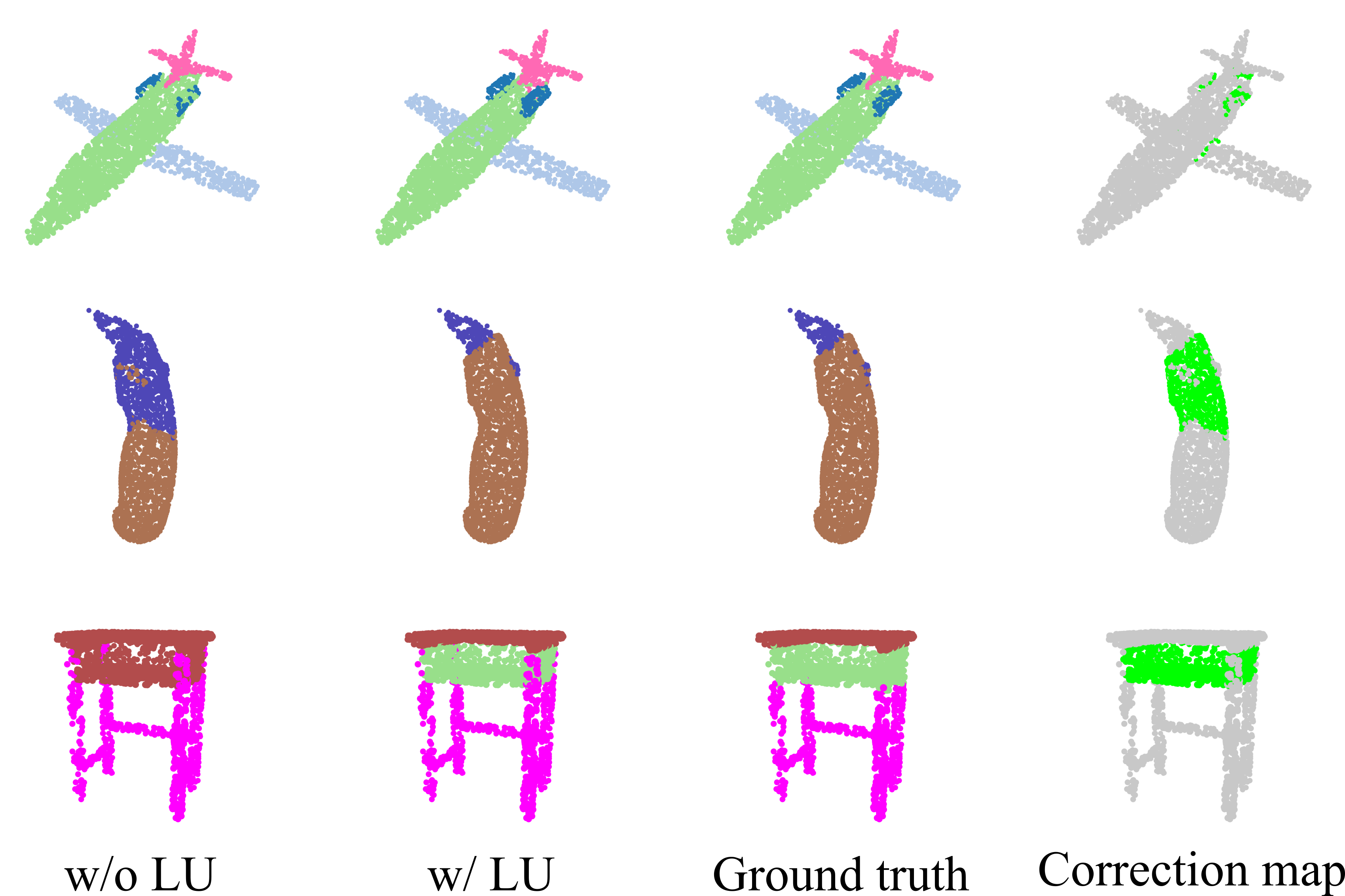
The results are reported in Table 2. As can be seen, LU-CNN achieves competitive performance compared with recent works. By applying LUs to our plain network, the performance is significantly improved by 0.4 ImIoU and 0.7 CmIoU points, successfully demonstrating the effectiveness of LU. As shown in the first row of Fig. 4, LU-CNN produces more precise predictions in near boundary regions compared to the plain counterpart. Therefore, LUs are especially effective in locating object boundaries. This point is also verified in the second row of Fig. 4 in which LU-CNN manages to detect very subtle changes of the surface and prevents over-smoothing. In contrast to the plain network which is confused by similar parts (e.g., tabletop and drawer, the third row of Fig. 4), LU-CNN clearly identifies two parts as separated ones and produces more perceptually sound predictions. We conjecture that the recognition of boundaries helps the network to separate different parts. Although LU-CNN fails to outperform AGCN (Kim and Alexander, 2021) that adopts additional adversarial training, we observe that our network beats the plain AGCN (AGCN (No adv.) in Table 2) that trained under the similar setting as ours significantly. Therefore, we believe that LU-CNN is fairly competitive among recent strong methods under the similar training setting.
4.3 Scene Segmentation
Dataset
We use Stanford Large-Scale 3D Indoor Spaces (S3DIS) (Armeni et al., 2016) for scene segmentation. In total, six indoor environments (areas) containing 272 rooms are included. Each point is labeled with a class from 13 categories. The number of points contained in a room ranges from 0.2M to 4.5M. As suggested by (Tchapmi et al., 2017), we use Area-5 for testing and others for training.
Setting
Since most rooms contain over 1M points which are difficult to fit into the GPU memory, we voxelize and downsample each room with a resolution of 0.04 m. As a result, each mini-batch element consists of a point cloud that contains at most 80,000 points. During testing, we make sure that every point is evaluated. The input feature consists of 3D coordinates and colors. We use the SGD optimizer with an initial learning rate of 0.1. The learning rate is decayed by a factor of 10 when the number of epochs reaches 60 and 80. The model is trained for 100 epochs in total. Since we can crop arbitrary numbers of training samples from rooms, we manually set the number of iterations in each epoch to 400. The batch size is set to 16. We augment the input data using random anisotropic scaling, random color translation, color jittering, and color translation in HSV space. Following prior works, we assess the performance using the point average IoU (mIoU), overall accuracy (OA), and mean accuracy (MA).
| Method | mIoU | OA | MA |
|---|---|---|---|
| PointCNN (Li et al., 2018b) | 57.3 | 85.9 | 63.9 |
| KPConv (Thomas et al., 2019) | 65.4 | - | 70.9 |
| KPConv deform (Thomas et al., 2019) | 67.1 | - | 72.8 |
| PointWeb (Zhao et al., 2019) | 60.3 | 87.0 | 66.6 |
| Minkowski (Choy et al., 2019) | 65.4 | - | 71.7 |
| BAAF-Net (Qiu et al., 2021b) | 65.4 | 88.9 | 73.1 |
| PAConv (Xu et al., 2021) | 66.6 | - | - |
| CGA-Net (Lu et al., 2021) | 68.6 | - | - |
| RFCR (Gong et al., 2021) | 68.7 | - | - |
| Point Transformer (Zhao et al., 2021) | 70.4 | 90.8 | 76.5 |
| Ours (w/o LU) | 68.3 | 90.5 | 74.8 |
| Ours | 69.6 | 90.7 | 75.9 |

Result
The result of scene segmentation is reported in Table 3. LU-CNN achieves the second-best performance among recent strong methods. Although our plain network fails to compete with the recent cutting-edge networks, LUs significantly advance its performance by 1.3 mIoU, 0.2 OA, and 1.1 MA points, respectively. The primary effect of LU is the accurate localization of object boundaries. As can be seen in the correction map of the first row of Fig. 5, the improvement is shown in near-boundary areas, making predictions more faithful to the ground truth. Secondly, owing to its ability to perform adaptive smoothing, the network with LUs, in general, produces smoother predictions. For instance, the fourth row of Fig. 5 shows that not only the boundary of the window is recognized precisely but also the predictions of the within-boundary region present a smoother distribution compared to the one without LUs. Furthermore, with the increased sensitivity to the geometrical/semantic changes of the surface, the network with LUs detects objects that are completely ignored by the plain counterpart and considerably improves the predictions both qualitatively and quantitatively (e.g., the second row of Fig. 5). We believe that giving the freedom to perform smoothing or sharpening to LU makes the network more aware of the connectivity of the underlying surface, thus making predictions smoother within and sharper near object boundaries.
4.4 Ablation study
In this section, a wide range of experiments are conducted to investigate the design choices of LU. Specifically, we perform the component analysis to validate the influence of each component w.r.t the final performance. Next, the generalization ability of LU with regard to different local operators is assessed. All experiments are performed on the part segmentation task because we believe that the effect of adaptive local feature learning is significant in this task as analyzed in Sec. 4.2.
4.4.1 Component analysis
Transformations and
Both transformations together transform the raw discrete Laplacian into the learnable one as defined in Eq. (6). In other words, they are responsible for adaptively smoothing or sharpening the features so as to improve the performance. As shown in Table 4, the networks (Model B and C) achieve degraded performance when either of them is removed. Notice that the Model B and C still able to improve over the baseline; thus, each function has a favorable effect on the overall performance. Removing both mappings (Model D) obtain significantly reduced performance whereas the full network (Model A) outperforms the Model B and C, demonstrating that both components work jointly to achieve the best performance.
| Model | Fusion | ImIoU | |||
|---|---|---|---|---|---|
| Baseline | - | - | - | - | 86.1 |
| A | ✓ | ✓ | Add. | 16 | 86.7 |
| B | ✓ | Add. | 16 | 86.4 | |
| C | ✓ | Add. | 16 | 86.4 | |
| D | Add. | 16 | 85.5 | ||
| E | ✓ | ✓ | Concat. | 16 | 86.5 |
| F | ✓ | ✓ | Mul. | 16 | 68.1 |
| G | ✓ | ✓ | 16 | 85.4 | |
| H | ✓ | ✓ | Add. | 8 | 86.5 |
| I | ✓ | ✓ | Add. | 24 | 86.5 |
| J | ✓ | ✓ | Add. | 32 | 86.7 |
Local-global fusion method
To combine the local feature and the global feature, we use the addition (Add.) fusion in LU by default because the addition naturally appears in the decomposed filtering equation (Eq. (2)). Moreover, addition also makes the relationship between LU and mean curvature flow straightforward (Sec. 3.2.2). However, one may conjecture that other fusion methods are also effective. Therefore, we explore two popular fusion methods: the concatenation (Concat.) (Wang et al., 2019b) (Model E) and multiplication (Mul.) (Hu et al., 2018) (Model F). Additionally, we also present the result without any fusion, i.e., in Eq. (7) is treated as the output of LU. The results are shown in Table 4. Obviously, the Add. is a particular solution of the Concat., and thus the Concat. should at least be not inferior to Add.. We find that, however, Concat. degrades the performance by 0.2, which contradicts our intuition. The reason for this might be due to the difficulty of joint optimization of local and global components. Moreover, we believe that it is challenging for the solver to exactly approximate the Add.. Further, the more expressive Concat. falls short of simple Add. proves that our design choice is more effective. On the other hand, Mul. degrades the performance significantly. Mul. fusion multiplies the global and local representations, which makes the backpropagated gradients for local and global features be tied together. We believe that too many interactions between two representations during optimization can increase the optimization difficulty as they represent fairly different properties of a point.
Number of neighbors
We vary the number of neighbors involved in LU to investigate its impact. is varied from 8 to 32. The results are shown in Table 4. The best performance are reached when is 16 (Model A) or 32 (Model J) whereas the performance drop when is set to 8 (Model H) or 24 (Model I). Therefore, we adopt 16 as the default choice.
4.4.2 LU with various local operators
| Local operator | w/o LU | w/ LU | |
|---|---|---|---|
| PointNet++ (Qi et al., 2017b) | 85.1 | 85.5 | +0.4 |
| PointConv (Wu et al., 2019) | 86.3 | 86.7 | +0.4 |
| RSCNN (Liu et al., 2019) | 85.9 | 86.2 | +0.3 |
| KPConv (Thomas et al., 2019) | 86.2 | 86.3 | +0.1 |
| KPConv-DS (Ours) | 86.1 | 86.7 | +0.6 |
We explore the impact of LU on different networks by varying the local operators. Specifically, we fix our backbone architecture and replace the KPConv-DS with other local operators to construct different networks. Four widely used local operators are chosen and evaluated. Then, we compare the performance before and after adding LUs to architectures. The results are reported in Table 5. Results show that LU can consistently provide performance improvement for different networks, demonstrating its general applicability. Notably, KPConv-DS (Ours) achieves similar performance as KPConv (Thomas et al., 2019), showing the effectiveness of our modifications on KPConv.
4.5 Computational complexity
| #LU | No | 2 | 4 | 6 | Full (18) |
|---|---|---|---|---|---|
| #param.(M) | 6.76 | 6.78 | 6.82 | 6.95 | 11.33 |
| Speed (ms) | 22.9 | 23.7 | 24.3 | 24.8 | 27.4 |
| ImIoU | 86.1 | 86.3 | 86.5 | 86.5 | 86.7 |
In this section, we analyze the additional parameters and inference time caused by combining LUs on part segmentation. In particular, we gradually increase the number of LU in the LU-CNN by adding a pair of LUs to the end of each stage. For instance, when the number of LU is set to two, a pair of LUs are added to the end of stage one in the encoder and the decoder simultaneously. The number of LU is then gradually increased from 0 to full to measure accuracy-complexity trade-offs. The results are listed in Table 6. As can be seen, the increase of parameters and the inference time introduced by LUs are marginal when #LU. is set to 2–6. On the other hand, the performance approaches the one of the Full model (86.7) quickly as it achieves 86.5 when #LU. is only 6. In general, we observe that the performance improvement brought by LU is efficient when #LU is low while the improvement saturates and becomes incremental when #LU becomes greater. Therefore, the efficient use of computational resources can be realized by limiting the number of LUs to be small to meet the specific requirement at hand.
4.6 Visual interpretation of LU by curvature analysis


In this section, we provide qualitative analysis concerning the underlying mechanism of LU and explain how LU improves performance. As we describe in Sec. 3.2.2, the behavior of LU can be investigated by analyzing the change of curvatures. Specifically, we measure the impact of LU by inspecting the change of curvatures qualitatively before and after applying LU. Three quantities are used for analysis: the input curvature , the output curvature , and . Comparing with reveals the effect of LU on the smoothness of local surfaces. Furthermore, contrasting and shows more directly how LU transforms the local features. We use the ShapeNet (part segmentation) and S3DIS (scene segmentation) for the analysis. The results are shown in Fig. 6 and Fig. 7, respectively.
As indicated by the yellow arrows in Fig. 6 and 7, LU performs smoothing in some cases just as indicated by its connection to mean curvature flow. As can be seen from the first row of Fig. 7, for instance, small variations on the ceiling and the wall of the room are smoothed. Notice that LU does not blindly smooth out everything; in fact, we observe that the sharp edges of the objects remain salient while within-boundary regions are smoothed. Therefore, LU is able to perform smoothing selectively.
On the other hand, as can be seen from the second rows of Fig. 6 and Fig. 7, LU sharpens features by increasing their curvatures in some situations, which is in stark contrast to the mean curvature flow that only performs smoothing. More importantly, LU performs selective sharpening by increasing curvatures for some object edges whereas non-edge regions remain smooth. Furthermore, the fact that most sharpened edges correspond well to the ground truth object boundaries reveals that the effect of LU is task-dependent, further demonstrating its adaptability.
Apart from the cases where LU dominantly performs smoothing or sharpening, we observe that LU can simultaneously perform smoothing and sharpening to different parts of a single point cloud. Such situations are described by the last rows of Fig. 6 and Fig. 7. Scrutinizing and reveals that LU manages to remove small variations for intraregion points while enhancing points near object boundaries. Such an effect is more frequently observed in deeper layers where features are highly semantic.
5 Discussions
In designing LU, we especially put emphasis on its lightweightness and optimization friendliness; hence, the design choice adopted in this study is fairly simple and computationally efficient. However, it is highly likely that more sophisticated designs of mappings and may provide performance improvements at the cost of reduced efficiency. We thus believe that there exists much space to extend its design so that the developed variant can be tailored to a specific kind of point clouds or task. One interesting direction would be the combination of LU and attention mechanism (Vaswani et al., 2017) in which neighborhood relationship is modeled adaptively. We expect that dynamically constructing the neighborhood graph would result in enhanced robustness against common problems like inconsistent neighborhood or measurement noise.
Although LU has limited impact on tasks like classification in which globally aggregated information matters, LU provides a significant improvement on more challenging segmentation tasks. Therefore, LU is expected to be rather helpful for tasks involving per-point labelings such as object detection and instance segmentation, which is the direction that we will explore in the future. Furthermore, we believe that LU is especially more influential in applications that require more fine-grained modeling of the local surface geometry. An interesting example of such applications is building damage classification (Xiu et al., 2020) where damage manifested itself as locally deformed surfaces.
6 Conclusion
The fact that a point cloud lacks connectivity information makes it challenging to analyze the geometry of the underlying surface. To tackle this issue, this study proposes a simple yet effective architectural unit called Laplacian Unit (LU) that facilitates the learning of local surface geometry. Observing that the convolution equation consists of coupled modeling of local and global components, LU explicitly decouples their shared optimization and enhances the local feature learning by applying independent transformations to local components. Further, the networks equipped with LUs, namely LU-CNNs, are constructed to tackle point cloud classification, part segmentation, and scene segmentation. Extensive experiments have verified that LU-CNNs achieve competitive or superior performance on several challenging benchmarks. In addition, the resulting form of LU enables us to establish straightforward connections between LU and mean curvature flow, an algorithm that smooths the surface using curvature information. We take advantage of such connections and visually interpret the behavior of LU by examining curvatures. As a result, we show by analysis that LU in effect performs adaptive smoothing and sharpening of local surfaces, which leads to improved performance. We believe LU, which explicitly decouples the convolution and enhances the learning of local geometry in an efficient and learning-friendly manner, can be a useful architectural unit for 3D point cloud understanding.
Acknowledgments
This work was partially supported by a project commissioned by the New Energy and Industrial Technology Development Organization (JPNP18010), JSPS Grant-in-Aid for Scientific Research (21K12042) and Fundamental Research Funds for the Central Universities under Grant DUT21RC(3)028.
References
- Armeni et al. (2016) Armeni, I., Sener, O., Zamir, A.R., Jiang, H., Brilakis, I., Fischer, M., Savarese, S., 2016. 3d semantic parsing of large-scale indoor spaces, in: Proceedings of the IEEE Conference on Computer Vision and Pattern Recognition, pp. 1534–1543.
- Atzmon et al. (2018) Atzmon, M., Maron, H., Lipman, Y., 2018. Point convolutional neural networks by extension operators. ACM Transactions on Graphics (TOG) 37, 1–12.
- Biasutti et al. (2019) Biasutti, P., Aujol, J.F., Brédif, M., Bugeau, A., 2019. Diffusion and inpainting of reflectance and height lidar orthoimages. Computer Vision and Image Understanding 179, 31–40.
- Chang et al. (2017) Chang, B., Meng, L., Haber, E., Tung, F., Begert, D., 2017. Multi-level residual networks from dynamical systems view. arXiv preprint arXiv:1710.10348 .
- Chollet (2017) Chollet, F., 2017. Xception: Deep learning with depthwise separable convolutions, in: Proceedings of the IEEE conference on computer vision and pattern recognition, pp. 1251–1258.
- Choy et al. (2019) Choy, C., Gwak, J., Savarese, S., 2019. 4d spatio-temporal convnets: Minkowski convolutional neural networks, in: Proceedings of the IEEE/CVF Conference on Computer Vision and Pattern Recognition, pp. 3075–3084.
- Cui et al. (2021) Cui, Y., Chen, R., Chu, W., Chen, L., Tian, D., Li, Y., Cao, D., 2021. Deep learning for image and point cloud fusion in autonomous driving: A review. IEEE Transactions on Intelligent Transportation Systems .
- Desbrun et al. (1999) Desbrun, M., Meyer, M., Schröder, P., Barr, A.H., 1999. Implicit fairing of irregular meshes using diffusion and curvature flow, in: Proceedings of the 26th annual conference on Computer graphics and interactive techniques, pp. 317–324.
- Feng et al. (2018) Feng, Y., Zhang, Z., Zhao, X., Ji, R., Gao, Y., 2018. Gvcnn: Group-view convolutional neural networks for 3d shape recognition, in: Proceedings of the IEEE Conference on Computer Vision and Pattern Recognition, pp. 264–272.
- Geiger et al. (2012) Geiger, A., Lenz, P., Urtasun, R., 2012. Are we ready for Autonomous Driving? The KITTI Vision Benchmark Suite, in: Proc. of the IEEE Conf. on Computer Vision and Pattern Recognition (CVPR), pp. 3354–3361.
- Glorot et al. (2011) Glorot, X., Bordes, A., Bengio, Y., 2011. Deep sparse rectifier neural networks, in: Proceedings of the fourteenth international conference on artificial intelligence and statistics, JMLR Workshop and Conference Proceedings. pp. 315–323.
- Gong et al. (2021) Gong, J., Xu, J., Tan, X., Song, H., Qu, Y., Xie, Y., Ma, L., 2021. Omni-supervised point cloud segmentation via gradual receptive field component reasoning, in: Proceedings of the IEEE/CVF Conference on Computer Vision and Pattern Recognition, pp. 11673–11682.
- Goyal et al. (2021) Goyal, A., Law, H., Liu, B., Newell, A., Deng, J., 2021. Revisiting point cloud shape classification with a simple and effective baseline. International Conference on Machine Learning .
- Graham et al. (2018) Graham, B., Engelcke, M., Van Der Maaten, L., 2018. 3d semantic segmentation with submanifold sparse convolutional networks, in: Proceedings of the IEEE conference on computer vision and pattern recognition, pp. 9224–9232.
- Guo et al. (2021) Guo, M.H., Cai, J.X., Liu, Z.N., Mu, T.J., Martin, R.R., Hu, S.M., 2021. Pct: Point cloud transformer. Computational Visual Media 7, 187–199.
- Hackel et al. (2017) Hackel, T., Savinov, N., Ladicky, L., Wegner, J.D., Schindler, K., Pollefeys, M., 2017. SEMANTIC3D.NET: A new large-scale point cloud classification benchmark, in: ISPRS Annals of the Photogrammetry, Remote Sensing and Spatial Information Sciences, pp. 91–98.
- Hamdi et al. (2021) Hamdi, A., Giancola, S., Ghanem, B., 2021. Mvtn: Multi-view transformation network for 3d shape recognition, in: Proceedings of the IEEE/CVF International Conference on Computer Vision, pp. 1–11.
- He et al. (2016) He, K., Zhang, X., Ren, S., Sun, J., 2016. Deep residual learning for image recognition, in: Proceedings of the IEEE conference on computer vision and pattern recognition, pp. 770–778.
- Howard et al. (2017) Howard, A.G., Zhu, M., Chen, B., Kalenichenko, D., Wang, W., Weyand, T., Andreetto, M., Adam, H., 2017. Mobilenets: Efficient convolutional neural networks for mobile vision applications. arXiv preprint arXiv:1704.04861 .
- Hu et al. (2018) Hu, J., Shen, L., Sun, G., 2018. Squeeze-and-excitation networks, in: Proceedings of the IEEE conference on computer vision and pattern recognition, pp. 7132–7141.
- Hua et al. (2018) Hua, B.S., Tran, M.K., Yeung, S.K., 2018. Pointwise convolutional neural networks, in: Proceedings of the IEEE Conference on Computer Vision and Pattern Recognition, pp. 984–993.
- Ioffe and Szegedy (2015) Ioffe, S., Szegedy, C., 2015. Batch normalization: Accelerating deep network training by reducing internal covariate shift, in: International conference on machine learning, PMLR. pp. 448–456.
- Kanezaki et al. (2018) Kanezaki, A., Matsushita, Y., Nishida, Y., 2018. Rotationnet: Joint object categorization and pose estimation using multiviews from unsupervised viewpoints, in: Proceedings of the IEEE Conference on Computer Vision and Pattern Recognition, pp. 5010–5019.
- Kim and Alexander (2021) Kim, S., Alexander, D.C., 2021. Agcn: Adversarial graph convolutional network for 3d point cloud segmentation. The 32nd British Machine Vision Conference .
- Krizhevsky et al. (2012) Krizhevsky, A., Sutskever, I., Hinton, G.E., 2012. Imagenet classification with deep convolutional neural networks. Advances in neural information processing systems 25, 1097–1105.
- Lan et al. (2019) Lan, S., Yu, R., Yu, G., Davis, L.S., 2019. Modeling local geometric structure of 3d point clouds using geo-cnn, in: Proceedings of the IEEE/CVF Conference on Computer Vision and Pattern Recognition, pp. 998–1008.
- LeCun et al. (2015) LeCun, Y., Bengio, Y., Hinton, G., 2015. Deep learning. nature 521, 436–444.
- Li et al. (2019) Li, G., Muller, M., Thabet, A., Ghanem, B., 2019. Deepgcns: Can gcns go as deep as cnns?, in: Proceedings of the IEEE/CVF international conference on computer vision, pp. 9267–9276.
- Li et al. (2018a) Li, Q., Han, Z., Wu, X.M., 2018a. Deeper insights into graph convolutional networks for semi-supervised learning, in: Thirty-Second AAAI conference on artificial intelligence.
- Li et al. (2022) Li, X., Zhang, L., Zhu, Z., 2022. Snapshotnet: Self-supervised feature learning for point cloud data segmentation using minimal labeled data. Computer Vision and Image Understanding 216, 103339.
- Li et al. (2018b) Li, Y., Bu, R., Sun, M., Wu, W., Di, X., Chen, B., 2018b. Pointcnn: Convolution on -transformed points, in: Proceedings of the 32nd International Conference on Neural Information Processing Systems, pp. 828–838.
- Liu et al. (2019) Liu, Y., Fan, B., Xiang, S., Pan, C., 2019. Relation-shape convolutional neural network for point cloud analysis, in: Proceedings of the IEEE/CVF Conference on Computer Vision and Pattern Recognition, pp. 8895–8904.
- Liu et al. (2020) Liu, Z., Hu, H., Cao, Y., Zhang, Z., Tong, X., 2020. A closer look at local aggregation operators in point cloud analysis, in: European Conference on Computer Vision, Springer. pp. 326–342.
- Lu et al. (2021) Lu, T., Wang, L., Wu, G., 2021. Cga-net: Category guided aggregation for point cloud semantic segmentation, in: Proceedings of the IEEE/CVF Conference on Computer Vision and Pattern Recognition, pp. 11693–11702.
- Ma et al. (2022) Ma, X., Qin, C., You, H., Ran, H., Fu, Y., 2022. Rethinking network design and local geometry in point cloud: A simple residual mlp framework. arXiv preprint arXiv:2202.07123 .
- Mao et al. (2019) Mao, J., Wang, X., Li, H., 2019. Interpolated convolutional networks for 3d point cloud understanding, in: Proceedings of the IEEE/CVF International Conference on Computer Vision, pp. 1578–1587.
- Maturana and Scherer (2015) Maturana, D., Scherer, S., 2015. Voxnet: A 3d convolutional neural network for real-time object recognition, in: 2015 IEEE/RSJ International Conference on Intelligent Robots and Systems (IROS), IEEE. pp. 922–928.
- Qi et al. (2018) Qi, C.R., Liu, W., Wu, C., Su, H., Guibas, L.J., 2018. Frustum pointnets for 3d object detection from rgb-d data, in: Proceedings of the IEEE conference on computer vision and pattern recognition, pp. 918–927.
- Qi et al. (2017a) Qi, C.R., Su, H., Mo, K., Guibas, L.J., 2017a. Pointnet: Deep learning on point sets for 3d classification and segmentation, in: Proceedings of the IEEE conference on computer vision and pattern recognition, pp. 652–660.
- Qi et al. (2017b) Qi, C.R., Yi, L., Su, H., Guibas, L.J., 2017b. Pointnet++: Deep hierarchical feature learning on point sets in a metric space. Advances in Neural Information Processing Systems 30.
- Qiu et al. (2021a) Qiu, S., Anwar, S., Barnes, N., 2021a. Geometric back-projection network for point cloud classification. IEEE Transactions on Multimedia .
- Qiu et al. (2021b) Qiu, S., Anwar, S., Barnes, N., 2021b. Semantic segmentation for real point cloud scenes via bilateral augmentation and adaptive fusion, in: Proceedings of the IEEE/CVF Conference on Computer Vision and Pattern Recognition, pp. 1757–1767.
- Ronneberger et al. (2015) Ronneberger, O., Fischer, P., Brox, T., 2015. U-net: Convolutional networks for biomedical image segmentation, in: International Conference on Medical image computing and computer-assisted intervention, Springer. pp. 234–241.
- Sandler et al. (2018) Sandler, M., Howard, A., Zhu, M., Zhmoginov, A., Chen, L.C., 2018. Mobilenetv2: Inverted residuals and linear bottlenecks, in: Proceedings of the IEEE conference on computer vision and pattern recognition, pp. 4510–4520.
- Shen et al. (2018) Shen, Y., Feng, C., Yang, Y., Tian, D., 2018. Mining point cloud local structures by kernel correlation and graph pooling, in: Proceedings of the IEEE conference on computer vision and pattern recognition, pp. 4548–4557.
- Sheshappanavar and Kambhamettu (2021) Sheshappanavar, S.V., Kambhamettu, C., 2021. Dynamic local geometry capture in 3d point cloud classification, in: 2021 IEEE 4th International Conference on Multimedia Information Processing and Retrieval (MIPR), IEEE. pp. 158–164.
- Shinohara et al. (2020) Shinohara, T., Xiu, H., Matsuoka, M., 2020. Fwnet: Semantic segmentation for full-waveform lidar data using deep learning. Sensors 20, 3568.
- Sifre and Mallat (2014) Sifre, L., Mallat, S., 2014. Rigid-motion scattering for texture classification. arXiv preprint arXiv:1403.1687 .
- Simonovsky and Komodakis (2017) Simonovsky, M., Komodakis, N., 2017. Dynamic edge-conditioned filters in convolutional neural networks on graphs, in: Proceedings of the IEEE conference on computer vision and pattern recognition, pp. 3693–3702.
- Sorkine (2006) Sorkine, O., 2006. Differential representations for mesh processing, in: Computer Graphics Forum, Wiley Online Library. pp. 789–807.
- Spivak (1975) Spivak, M., 1975. A comprehensive introduction to differential geometry. volume 4. Publish or Perish, Incorporated.
- Su et al. (2015) Su, H., Maji, S., Kalogerakis, E., Learned-Miller, E., 2015. Multi-view convolutional neural networks for 3d shape recognition, in: Proceedings of the IEEE international conference on computer vision, pp. 945–953.
- Taubin (1995) Taubin, G., 1995. A signal processing approach to fair surface design, in: Proceedings of the 22nd annual conference on Computer graphics and interactive techniques, pp. 351–358.
- Tchapmi et al. (2017) Tchapmi, L., Choy, C., Armeni, I., Gwak, J., Savarese, S., 2017. Segcloud: Semantic segmentation of 3d point clouds, in: 2017 international conference on 3D vision (3DV), IEEE. pp. 537–547.
- Thomas et al. (2019) Thomas, H., Qi, C.R., Deschaud, J.E., Marcotegui, B., Goulette, F., Guibas, L.J., 2019. Kpconv: Flexible and deformable convolution for point clouds, in: Proceedings of the IEEE/CVF International Conference on Computer Vision, pp. 6411–6420.
- Tomasi and Manduchi (1998) Tomasi, C., Manduchi, R., 1998. Bilateral filtering for gray and color images, in: Sixth international conference on computer vision (IEEE Cat. No. 98CH36271), IEEE. pp. 839–846.
- Uy et al. (2019) Uy, M.A., Pham, Q.H., Hua, B.S., Nguyen, T., Yeung, S.K., 2019. Revisiting point cloud classification: A new benchmark dataset and classification model on real-world data, in: Proceedings of the IEEE/CVF International Conference on Computer Vision, pp. 1588–1597.
- Vaswani et al. (2017) Vaswani, A., Shazeer, N., Parmar, N., Uszkoreit, J., Jones, L., Gomez, A.N., Kaiser, L., Polosukhin, I., 2017. Attention is all you need. arXiv preprint arXiv:1706.03762 .
- Wang et al. (2019a) Wang, L., Huang, Y., Hou, Y., Zhang, S., Shan, J., 2019a. Graph attention convolution for point cloud semantic segmentation, in: Proceedings of the IEEE/CVF Conference on Computer Vision and Pattern Recognition, pp. 10296–10305.
- Wang et al. (2018) Wang, S., Suo, S., Ma, W.C., Pokrovsky, A., Urtasun, R., 2018. Deep parametric continuous convolutional neural networks, in: Proceedings of the IEEE Conference on Computer Vision and Pattern Recognition, pp. 2589–2597.
- Wang et al. (2019b) Wang, Y., Sun, Y., Liu, Z., Sarma, S.E., Bronstein, M.M., Solomon, J.M., 2019b. Dynamic graph cnn for learning on point clouds. Acm Transactions On Graphics (tog) 38, 1–12.
- Wu et al. (2019) Wu, W., Qi, Z., Fuxin, L., 2019. Pointconv: Deep convolutional networks on 3d point clouds, in: Proceedings of the IEEE/CVF Conference on Computer Vision and Pattern Recognition, pp. 9621–9630.
- Xiang et al. (2021) Xiang, T., Zhang, C., Song, Y., Yu, J., Cai, W., 2021. Walk in the cloud: Learning curves for point clouds shape analysis, in: Proceedings of the IEEE/CVF International Conference on Computer Vision, pp. 915–924.
- Xiu et al. (2022) Xiu, H., Liu, X., Wang, W., Kim, K.S., Shinohara, T., Chang, Q., Matsuoka, M., 2022. Enhancing local feature learning for 3d point cloud processing using unary-pairwise attention. arXiv preprint arXiv:2203.00172 .
- Xiu et al. (2020) Xiu, H., Shinohara, T., Matsuoka, M., Inoguchi, M., Kawabe, K., Horie, K., 2020. Collapsed building detection using 3d point clouds and deep learning. Remote Sensing 12, 4057.
- Xu et al. (2021) Xu, M., Ding, R., Zhao, H., Qi, X., 2021. Paconv: Position adaptive convolution with dynamic kernel assembling on point clouds. arXiv preprint arXiv:2103.14635 .
- Yan et al. (2020) Yan, X., Zheng, C., Li, Z., Wang, S., Cui, S., 2020. Pointasnl: Robust point clouds processing using nonlocal neural networks with adaptive sampling, in: Proceedings of the IEEE/CVF Conference on Computer Vision and Pattern Recognition, pp. 5589–5598.
- Yang et al. (2019) Yang, J., Zhang, Q., Ni, B., Li, L., Liu, J., Zhou, M., Tian, Q., 2019. Modeling point clouds with self-attention and gumbel subset sampling, in: Proceedings of the IEEE/CVF Conference on Computer Vision and Pattern Recognition, pp. 3323–3332.
- Yi et al. (2016) Yi, L., Kim, V.G., Ceylan, D., Shen, I.C., Yan, M., Su, H., Lu, C., Huang, Q., Sheffer, A., Guibas, L., 2016. A scalable active framework for region annotation in 3d shape collections. ACM Transactions on Graphics (ToG) 35, 1–12.
- Zhang et al. (2019) Zhang, Z., Hua, B.S., Yeung, S.K., 2019. Shellnet: Efficient point cloud convolutional neural networks using concentric shells statistics, in: Proceedings of the IEEE/CVF International Conference on Computer Vision, pp. 1607–1616.
- Zhao et al. (2019) Zhao, H., Jiang, L., Fu, C.W., Jia, J., 2019. Pointweb: Enhancing local neighborhood features for point cloud processing, in: Proceedings of the IEEE/CVF Conference on Computer Vision and Pattern Recognition, pp. 5565–5573.
- Zhao et al. (2021) Zhao, H., Jiang, L., Jia, J., Torr, P.H., Koltun, V., 2021. Point transformer, in: Proceedings of the IEEE/CVF International Conference on Computer Vision, pp. 16259–16268.
- Zhou and Tuzel (2018) Zhou, Y., Tuzel, O., 2018. Voxelnet: End-to-end learning for point cloud based 3d object detection, in: Proceedings of the IEEE Conference on Computer Vision and Pattern Recognition, pp. 4490–4499.
- Zhu et al. (2017) Zhu, X.X., Tuia, D., Mou, L., Xia, G.S., Zhang, L., Xu, F., Fraundorfer, F., 2017. Deep learning in remote sensing: A comprehensive review and list of resources. IEEE Geoscience and Remote Sensing Magazine 5, 8–36.