Enhancing interval observers for state estimation using constraints ^††thanks: This work was funded by Novartis Pharmaceuticals as part of the Novartis-MIT Center for Continuous Manufacturing.

First, notation that is used in this work includes lowercase bold letters for vectors and uppercase bold letters for matrices. The transposes of a vector $\mathbf{v}$ and matrix $\mathbf{M}$ are denoted $\mathbf{v}^{\textnormal{T}}$ and $\mathbf{M}^{\textnormal{T}}$, respectively. The exception is that $\mathbf{0}$ may denote either a matrix or vector of zeros, but it should be clear from context what the appropriate dimensions are. Similarly, $\mathbf{1}$ denotes a vector of ones whose dimension should be clear from context. The $j^{th}$ component of a vector $\mathbf{v}$ will be denoted ${v}_{j}$. For a matrix $\mathbf{M}\in\mathbb{R}^{p\times n}$, the notation $\mathbf{M}=[\mathbf{m}_{i}^{\textnormal{T}}]$ may be used to emphasize that the $i^{th}$ row of $\mathbf{M}$ is $\mathbf{m}_{i}$, for $i\in\{1,\dots,p\}$. Similarly, $\mathbf{M}=[m_{i,j}]$ emphasizes that the element in the $i^{th}$ row and $j^{th}$ column is $m_{i,j}$. Inequalities between vectors hold componentwise. For $\mathbf{v}$, $\mathbf{w}\in\mathbb{R}^{n}$ such that $\mathbf{v}\leq\mathbf{w}$, $[\mathbf{v},\mathbf{w}]$ denotes a nonempty interval in $\mathbb{R}^{n}$. For a set $Y\subset\mathbb{R}^{n}$, denote the set of nonempty interval subsets of $Y$ by $\mathbb{I}Y$. The equivalence of norms on $\mathbb{R}^{n}$ is used often; when a statement or result holds for any choice of norm, it is denoted $\left\|\cdot\right\|$. In some cases, it is useful to reference a specific norm, in which case it is subscripted; for instance, $\left\|\cdot\right\|_{1}$ denotes the 1-norm. The dual norm of a norm $\left\|\cdot\right\|$ is denoted $\left\|\cdot\right\|_{*}$. In a metric space, a neighborhood of a point $x$ is denoted $N(x)$ and refers to an open ball centered at $x$ with some nonzero radius.

The problem of interest is one in estimating the state of a continuous-time dynamic system; in particular, we seek a rigorous enclosure of the states or a bounded error estimate. The dynamic model of the system is defined by: for positive integers $n_{x},n_{y},n_{u}$, nonempty interval $T=[t_{0},t_{f}]\subset\mathbb{R}$, $D_{x}\subset\mathbb{R}^{n_{x}}$, $D_{u}\subset\mathbb{R}^{n_{u}}$, $\mathbf{f}:T\times D_{u}\times D_{x}\to\mathbb{R}^{n_{x}}$, and $\mathbf{C}\in\mathbb{R}^{n_{y}\times n_{x}}$. The system obeys the following equations:

where $\mathbf{x}(t)$ is the state of the system, $\mathbf{y}(t)$ is the measurement or output of the system, $\mathbf{u}(t)$ is a disturbance to the system, and $\mathbf{v}(t)$ is the measurement noise.

In this work, we exclusively consider absolutely continuous solutions $\mathbf{x}$ of the IVP in ODEs (1a). Further, we assume that it is known that the initial conditions satisfy $\mathbf{x}(t_{0})\in X_{0}\in\mathbb{I}D_{x}$, $\mathbf{v}$ is measurable and $\mathbf{v}(t)\in V(t)\in\mathbb{I}\mathbb{R}^{n_{y}}$ for all $t\in T$, $\mathbf{u}$ is measurable and $\mathbf{u}(t)\in U(t)\in\mathbb{I}D_{u}$ for all $t\in T$, where $V(t)\subset K_{v}$ and $U(t)\subset K_{u}$, for all $t\in T$, for compact $K_{v}$ and $K_{u}$. In other words, interval enclosures of the possible initial conditions, measurement noise, and disturbance values are known. A fundamental assumption on the dynamics $\mathbf{f}$ is a kind of local Lipschitz condition: For any $\mathbf{z}\in D_{x}$, there exists a neighborhood $N(\mathbf{z})$ and $\alpha\in L^{1}(T)$ such that for almost every $t\in T$ and every $\mathbf{w}\in U(t)$

for every $\mathbf{z}_{1},\mathbf{z}_{2}\in N(\mathbf{z})\cap D_{x}$.

The challenge, then is to construct an interval $[\mathbf{x}^{L}(t_{f}),\mathbf{x}^{U}(t_{f})]$ such that

for any possible realization of noise $\mathbf{v}$, disturbance $\mathbf{u}$, and initial condition.

For future reference, since $V$ and $U$ are interval-valued, we can write $V(t)=[\mathbf{v}^{L}(t),\mathbf{v}^{U}(t)]$ and $U(t)=[\mathbf{u}^{L}(t),\mathbf{u}^{U}(t)]$ for appropriate functions.

Previous work on bounded-error state estimation includes interval observers; we refer to [4] for a recent review of such work and some related topics. The essence of this type of method is easily understood for a linear system. Consider

Then for any matrix $\mathbf{L}\in\mathbb{R}^{n_{x}\times n_{y}}$, we can write

and subsequently

The theory of interval observers often focuses on the case that the “gain matrix” $\mathbf{L}$ is chosen so that $\mathbf{A}-\mathbf{LC}$ has positive off-diagonal components, and that $\left\|\mathbf{w}\right\|_{\infty}\leq v^{N}$, for all $\mathbf{w}\in V(t)$, for all $t$ (so that $\mathbf{L}\mathbf{v}(t)\leq\left\|\mathbf{L}\mathbf{v}(t)\right\|_{\infty}\mathbf{1}\leq\left\|\mathbf{L}\right\|_{\infty}v^{N}\mathbf{1}$, implying $-\left\|\mathbf{L}\right\|_{\infty}v^{N}\mathbf{1}\leq\mathbf{L}\mathbf{v}(t)\leq\left\|\mathbf{L}\right\|_{\infty}v^{N}\mathbf{1}$). In this case one can write

Then assuming $X_{0}\subset[\mathbf{x}^{L}(t_{0}),\mathbf{x}^{U}(t_{0})]$, the theory of monotone dynamic systems ensures that for any initial condition and realization of measurement noise, $\mathbf{x}(t)\in[\mathbf{x}^{L}(t),\mathbf{x}^{U}(t)]$, for all $t\in T$.

Our approach is to extend this idea with more general theorems for reachability analysis based on the theory of differential inequalities, and in particular, to leverage the recent developments that take advantage of constraint information to tighten the estimates of the reachable sets. To this end, we interpret the state estimation problem as a reachability problem for an IVP in constrained ODEs. This has been considered most recently in [8]. Similar techniques from [9, 7, 24] also apply; those articles use “a priori enclosures” of the reachable set, which are in effect constraints, although they do not necessarily exclude any solutions. As demonstrated in [8], these techniques can be applied to constrained systems, if one is only interested in solutions that also satisfy the constraints.

Thus, the proposed approach is to apply reachability analysis to the system

for some choice of matrix $\mathbf{L}$, and constraint mapping $X_{c}$ defined by $X_{c}(t)=\{\mathbf{z}:\mathbf{y}(t)-\mathbf{v}^{U}(t)\leq\mathbf{C}\mathbf{z}\leq\mathbf{y}(t)-\mathbf{v}^{L}(t)\}$.

Recent developments in the design of interval observers from [5, 26] allow the gain matrix $\mathbf{L}$ to vary, depending on time and measurements. There is no significant hurdle to incorporating such a generalization in the method that follows; we choose not to do so in order to keep notation simple and to highlight the essence of our contribution.

To state the method, we must introduce a few definitions and operations. Central to the method for estimating reachable sets that we will use, from [24], is the ability to overestimate or bound the dynamics. We will do so with an inclusion function constructed using principles from interval arithmetic. See [22] for an introduction to interval arithmetic and inclusion functions. As in the discussion above, the dynamics we care about are for a modified system depending on the gain matrix $\mathbf{L}$.

The critical property of an inclusion monotonic interval extension is that it is an inclusion function; that is

for any $U^{\prime}\in\mathbb{I}D_{u}$, $Z^{\prime}\in\mathbb{I}D_{x}$, $V^{\prime}\in\mathbb{IR}^{n_{y}}$, and $(t,\mathbf{u},\mathbf{z},\mathbf{v})\in T\times U^{\prime}\times Z^{\prime}\times V^{\prime}$. Inclusion functions for a broad class of functions can be automatically and cheaply evaluated with a number of numerical libraries implementing interval arithmetic, for instance, MC++ [2], INTLAB [23], or PROFIL [14]. The proposed method relies on these automatically computable inclusion functions, which reduces the amount of analysis that must be performed compared to other work. For instance, the work in [19, 18] requires analysis of the dynamics to derive a hybrid automata which is then used to construct the state estimate.

Since it will be useful later, we mention that the natural interval extension of a function is an inclusion monotonic interval extension. For a linear function $g:\mathbf{z}\mapsto\mathbf{a}^{\textnormal{T}}\mathbf{z}$, the natural interval extension $[g^{L},g^{U}]$ is computed by applying the rules of interval arithmetic:

We will also require the following definition. If $\mathbf{v}\leq\mathbf{w}$, then $B_{i}^{L}(\mathbf{v},\mathbf{w})$ returns the $i^{th}$ lower face of the interval $[\mathbf{v},\mathbf{w}]$. If $[\mathbf{v},\mathbf{w}]$ is empty, then a nonempty interval $[\widehat{\mathbf{v}},\widehat{\mathbf{w}}]$ is constructed and the faces of that interval are returned.

The operation defined in Algorithm 1 is required. Originally from Definition 4 in [24], this algorithm defines the operation $I_{t}$, which tightens an interval $[\mathbf{v},\mathbf{w}]$ by excluding points which cannot satisfy a given set of linear constraints $\mathbf{M}\mathbf{z}\leq\mathbf{d}$. Specifically, the discussion in §5.2 of [24] establishes that the tightened interval $I_{t}([\mathbf{v},\mathbf{w}],\mathbf{d};\mathbf{M})$ satisfies

With the definition of the interval tightening operator, we can define an operation specific to our problem which tightens an interval based on the constraints $\mathbf{C}\mathbf{z}\leq\mathbf{y}(t)-\mathbf{v}^{L}(t)$, $\mathbf{C}\mathbf{z}\geq\mathbf{y}(t)-\mathbf{v}^{U}(t)$.

We can now state the specific method for constructing a state estimator. The main difference between this method and a classic comparison theorem for reachability (see [6]) is the application of the $I_{c}$ operator. While the classic method would overstimate, for instance, $\widehat{f}_{i}$ on the set $\{\mathbf{z}\in[\mathbf{x}^{L}(t),\mathbf{x}^{U}(t)]:z_{i}=x_{i}^{U}(t)\}$ (the $i^{th}$ upper face of the interval), the proposed method applies $I_{c}$ to that set, and overestimates $\widehat{f}_{i}$ on the resulting (no larger) interval.

We note that Theorem 1 does not guarantee the existence of $\mathbf{x}^{L}$ and $\mathbf{x}^{U}$; it provides a construction that, if successful, yields an interval estimate. Conditions that we have not stated explicitly, such as continuity of $\widehat{\mathbf{f}}^{L}$ and $\widehat{\mathbf{f}}^{U}$ and measurability of $\mathbf{v}^{L}$, $\mathbf{v}^{U}$, $\mathbf{u}^{L}$, $\mathbf{u}^{U}$ (defining the set-valued mappings $V$ and $U$), may be required to apply standard existence results for the solutions of IVPs in ODEs. Perhaps more important are the typically stronger conditions that guarantee the applicability of numerical methods for the solution of IVPs in ODEs; see, for instance, Theorem 1.1 of Section 1.4 of [17]. For example, in the numerical examples that follow, we use measurements $\mathbf{y}$ that are a continuous function on $T$.

In §4, we will compare the proposed method established above against its variants and others from the literature. The method from Theorem 1 with $\mathbf{L}=\mathbf{0}$ is called the “No Measurements” method; while it still uses measurement information as constraints, it does not use the measurement values $\mathbf{y}(t)$ directly. Meanwhile, the “No Constraints” method is a variant of the proposed method that does not use the constraint information; that is, the endpoints of the interval estimate satisfy the differential equations

Note that application of the operation $I_{c}$ has been omitted.

Methods from the literature for calculating the gain matrix $\mathbf{L}$ often focus on the case that the system is linear, e.g. $\dot{\mathbf{x}}=\mathbf{A}\mathbf{x}$. The methods often involve finding a gain matrix $\mathbf{L}$ so that $\mathbf{A}-\mathbf{LC}$ has nonnegative off-diagonal components; a matrix with this last property is often called a Metzler matrix. Consequently, the theory of cooperative or monotone systems can be applied to derive interval estimates.

In the present section, our goal is to state a method for calculating the gain matrix that does not depend on the system being cooperative. We begin with a fundamental result which will motivate the method; we show that the No Constraints method with a gain matrix satisfying certain constraints will produce an asymptotically exact interval estimate for an idealized linear system.

Related results are in the literature, like [4, Thm. 1]. Stability/asymptotic properties of the interval state estimate are often stated as requiring $\mathbf{A}-\mathbf{LC}$ to have eigenvalues with negative real part; it is clear, again using Gershgorin’s circle theorem, that conditions (4), if satisfied, imply exactly this. Of course, it is not the stability of the modified system $\dot{\mathbf{x}}=(\mathbf{A}-\mathbf{LC})\mathbf{x}+\mathbf{L}\mathbf{y}$ that matters – this is mostly a coincidence; it is the stability of the dynamics defining $\mathbf{x}^{U}-\mathbf{x}^{L}$ that determines their asymptotic properties.

To turn the conditions in Theorem 2 into an implementable numerical procedure, the next result states that a gain matrix satisfying the conditions may be found as the solution of a linear program (LP).

As a practical note, we would add a (negative) lower bound on $s$ to the above LP in order to prevent the possibility that the LP is unbounded. Further, the variables $b_{i,i}$ do not appear in the constraints or objective and could be eliminated; a decent numerical LP solver will likely identify this automatically and eliminate them in a presolve step.

Other results for calculating the gain matrix based on the solution of an LP have been proposed; see for instance [3]. Again, these results rely on something like $\mathbf{A}-\mathbf{LC}$ being Metzler, although this extra structure permits more detailed claims about the input-output gains of the system.

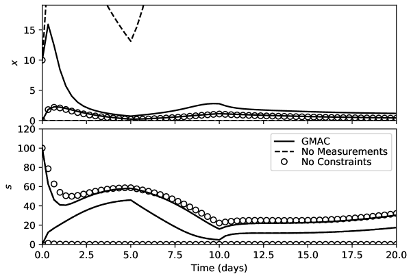
We consider an example involving a bioreactor originally from [20, 19]. The dynamic model describes the evolution in time of the concentrations of biomass and feed substrate. The dynamic equations on the time domain $T=[0,20]$ (day) are

where $x(t)$ and $s(t)$ are the biomass and substrate concentrations, respectively, at time $t$, and the known parameters are

Meanwhile, the unknown parameters/disturbances are $(\mu_{0},s_{in})$ which satisfy for all $t\in T$

where $\widehat{s}_{in}:t\mapsto 50+15\cos(t/5)$ (so take $U:t\mapsto[0.703,0.777]\times[0.95\widehat{s}_{in}(t),1.05\widehat{s}_{in}(t)]$).

Continuous measurements of $x(t)$, the biomass concentration, are available (so $\mathbf{C}=[1\;0]$). The error¹¹1We note that the error in the initial measurements of the biomass concentration are much larger than the subsequent measurements. While in practice it seems likely that the initial measurements should be known at least as accurately as any subsequent online measurements, for consistency we follow this example as it appears in [20, 19]. in these measurements satifies $v(t)\in[-0.25,0.25]$. For simulation purposes, we obtain measurements from a numerical solution with $\mu_{0}(t)=0.74$ for all $t$, $s_{in}(t)=\widehat{s}_{in}(t)$ for all $t$, $v(t)=0$ for all $t$, and initial conditions $x(0)=5$ and $s(0)=40$. These measurements are obtained at 500 equally spaced time points from the interval $T$, and then made continuous by linearly interpolating between them.

In [20], a “bundle” of interval observers are constructed, essentially by running independent estimates with different gain matrices $\mathbf{L}$. We choose one of these gain matrices $\mathbf{L}=[2\;0]^{\textnormal{T}}$.

Figure 1 summarizes the results; the upper and lower bounds of the interval estimate for each state is plotted versus time. The proposed GMAC method is strictly tighter than either the No Measurements or No Constraints methods for at least one of the states. The interval estimates at the final time are given in Table 1.

Compared to the bundle of observers from [20], the estimates from GMAC are of comparable quality. As mentioned, however, we achieve our results with only one observer gain matrix. The same example is considered in [19], and again we achieve similar state estimates. The work in [19] is based on a hybrid automata approach, and some extra analysis to determine the switching conditions is required. Meanwhile, we rely on automatic construction of inclusion functions through implementations of interval arithmetic and little extra analysis is required.

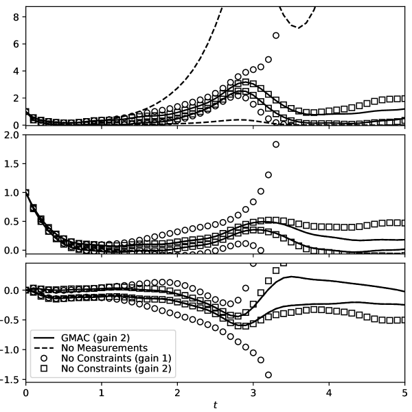
This example comes from Example 1 of [4]. We have a three state system with nonlinear dynamics; $\mathbf{x}$ satisfies

where

The time interval of interest is $T=[0,5]$, with the state known at $t=0$: $\mathbf{x}(0)=(1,1,0)$. The disturbances satisfy $(u_{1}(t),u_{2}(t))\in[4.48,6.12]\times[3.2,3.6]$. Measurements of the first state are available, so that $\mathbf{C}=[1\;0\;0]$. The error in these measurements satisfies $v(t)\in[-0.1,0.1]$. For simulation purposes, we obtain measurements from a numerical solution of the system with $u_{1}(t)=5.3$ for all $t$, $u_{2}(t)=3.4$ for all $t$, and $v(t)=0.1\sin(10t)$. These measurements are obtained at 500 equally spaced time points from the interval $T$, and then made continuous by linearly interpolating between them.

Although this is a nonlinear system, we attempt to design an observer gain matrix based on the linear part. The original analysis in [4, Example 1] suggests

However, solving LP (7) yields

and a negative optimal objective value is obtained. We will calculate state estimates with both separately. Refer to these as “gain 1” and “gain 2,” respectively. Recall that the No Measurements method is defined by using $\mathbf{L}=\mathbf{0}$, and so it remains the same.

Figure 2 summarizes the results; the upper and lower bounds of the interval estimate for each state is plotted versus time. For this example, omitting constraints produces a much more conservative interval state estimate. In fact, the bounds produced by the No Constraints method with gain 1 diverge and the numerical integration procedure prematurely terminates shortly after $t=3.5$ (specifically, the corrector iteration of the BDF in CVODE fails). Using gain 2, the No Constraints method performs much better and can produce state estimates for the entire time interval.

Meanwhile, the proposed GMAC method (with either gain- the results are largely the same) more consistently produces a tight interval estimate for each state. The No Measurements method is comparable. Table 2 lists specific values at the final time. The main difference is that the estimate of the first state from GMAC is much tighter. This is somewhat of a moot point, however, as bounded-error measurements of the first state are directly available; for our simulated measurement values, this implies the interval estimate $x_{1}(5)\in[0.692,0.892]$.

References

- [1] Olivier Bokanowski, Nicolas Forcadel, and Hasnaa Zidani. Reachability and minimal times for state constrained nonlinear problems without any controllability assumption. SIAM Journal on Control and Optimization, 48(7):4292–4316, 2010.
- [2] Benoît Chachuat. MC++: A Versatile Library for McCormick Relaxations and Taylor Models. http://www.imperial.ac.uk/people/b.chachuat/research.html, 2015.
- [3] Stanislav Chebotarev, Denis Efimov, Tarek Raïssi, and Ali Zolghadri. Interval observers for continuous-time lpv systems with l1/l2 performance. Automatica, 58:82–89, 2015.
- [4] Denis Efimov and Tarek Raïssi. Design of interval observers for uncertain dynamical systems. Automation and Remote Control, 77(2):191–225, 2016.
- [5] Denis Efimov, Tarek Raïssi, Stanislav Chebotarev, and Ali Zolghadri. Interval state observer for nonlinear time varying systems. Automatica, 49(1):200–205, 2013.
- [6] Gary W. Harrison. Dynamic models with uncertain parameters. In X .J. R. Avula, editor, Proceedings of the First International Conference on Mathematical Modeling, volume 1, pages 295–304. University of Missouri Rolla, 1977.
- [7] Stuart M. Harwood and Paul I. Barton. Efficient polyhedral enclosures for the reachable set of nonlinear control systems. Mathematics of Control, Signals, and Systems, 28(1):8, 2016.
- [8] Stuart M. Harwood and Paul I. Barton. Affine relaxations for the solutions of constrained parametric ordinary differential equations. Optimal Control Applications and Methods, 2017.
- [9] Stuart M. Harwood, Joseph K Scott, and Paul I. Barton. Bounds on reachable sets using ordinary differential equations with linear programs embedded. IMA Journal of Mathematical Control and Information, 33(2):519–541, 2016.
- [10] Alan C. Hindmarsh, Peter N. Brown, Keith E. Grant, Steven L. Lee, Radu Serban, Dan E. Shumaker, and Carol S. Woodward. SUNDIALS: Suite of Nonlinear and Differential/Algebraic Equation Solvers. ACM Transactions on Mathematical Software, 31(3):363–396, 2005.
- [11] L. Jaulin. Nonlinear bounded-error state estimation of continuous-time systems. Automatica, 38(6):1079–1082, 2002.
- [12] R. E. Kalman. A New Approach to Linear Filtering and Prediction Problems. Journal of Basic Engineering, 82:35–45, 1960.
- [13] Hassan K. Khalil. Nonlinear Systems. Prentice-Hall, Upper Saddle River, NJ, second edition, 1996.
- [14] O. Knüppel. PROFIL/BIAS — A fast interval library. Computing, 53(3):277–287, Sep 1994.
- [15] A. B. Kurzhanski, I. M. Mitchell, and P. Varaiya. Optimization techniques for state-constrained control and obstacle problems. Journal of Optimization Theory and Applications, 128(3):499–521, 2006.
- [16] A. B. Kurzhanski and P. Varaiya. Ellipsoidal techniques for reachability under state constraints. SIAM Journal on Control and Optimization, 45(4):1369–1394, January 2006.
- [17] J. D. Lambert. Numerical Methods for Ordinary Differential Systems: The Initial Value Problem. John Wiley & Sons, New York, 1991.
- [18] N. Meslem and N. Ramdani. Interval observer design based on nonlinear hybridization and practical stability analysis. International Journal of Adaptive Control and Signal Processing, 25:228–248, 2011.
- [19] N. Meslem, N. Ramdani, and Y. Candau. Using hybrid automata for set-membership state estimation with uncertain nonlinear continuous-time systems. Journal of Process Control, 20:481–489, 2010.
- [20] M. Moisan and O. Bernard. Interval observers for non-montone systems. Application to bioprocess models. 16th IFAC World Congress, 16:43–48, 2005.
- [21] M. Moisan and O. Bernard. An interval observer for non-monotone systems: application to an industrial anaerobic digestion process. 10th International IFAC Symposium on Computer Applications in Biotechnology, 1:325–330, 2007.
- [22] Ramon E. Moore, R. Baker Kearfott, and Michael J. Cloud. Introduction to Interval Analysis. SIAM, Philadelphia, 2009.
- [23] Siegfried M. Rump. INTLAB — INTerval LABoratory. In Tibor Csendes, editor, Developments in Reliable Computing, pages 77–104. Springer Netherlands, Dordrecht, 1999.
- [24] Joseph K. Scott and Paul I. Barton. Bounds on the reachable sets of nonlinear control systems. Automatica, 49(1):93–100, 2013.
- [25] Gilbert Strang. Linear Algebra and its Applications. Thomson Brooks/Cole, fourth edition, 2006.
- [26] Rihab El Houda Thabet, Tarek Raïssi, Christophe Combastel, Denis Efimov, and Ali Zolghadri. An effective method to interval observer design for time-varying systems. Automatica, 50(10):2677–2684, 2014.
- [27] Wolfgang Walter. Differential and Integral Inequalities. Springer, New York, 1970.