Enhancing interferometry using weak value amplification with real weak values
Abstract
We introduce an ultra-sensitive interferometric protocol that combines weak value amplification (WVA) with traditional interferometry. This WVA+interferometry protocol uses weak value amplification of the relative delay between two paths to enhance the interferometric sensitivity, approaching the quantum limit for classical light. As an example, we demonstrate a proof-of-principle experiment that achieves few-attosecond timing resolution (few-nanometer path length resolution) with a double-slit interferometer using only common optical components. Since our example uses only the spatial shift of double-slit interference fringes, its precision is not limited by the timing resolution of the detectors, but is instead limited solely by the fundamental shot noise associated with classical light. We experimentally demonstrate that the signal-to-noise ratio can be improved by one to three orders of magnitude and approaches the shot-noise limit in the large amplification regime. Previously, quantum-limited WVA delay measurements were thought to require imaginary weak values, which necessitate light with a broad spectral bandwidth and high-resolution spectrometers. In contrast, our protocol highlights the feasibility of using real weak values and narrowband light. Thus, our protocol is a compelling and cost-effective approach to enhance interferometry.
Interferometry is widely used for making ultra-sensitive measurements of time delays. Examples include the Sagnac interferometer Eberle et al. (2010) for rotation-induced delays, the Mach-Zehnder interferometer Sorianello et al. (2018) for detecting refractive index changes in a sample, and Michelson interferometers for gravitational wave detection Abbott et al. (2016). Precise time delay estimations are also desired for pump-probe interferometry Nabekawa et al. (2009). Detecting few-nanometer path changes, which corresponds to attosecond time delay measurements, is a crucial tool in cellular biology and the study of monatomic layer two-dimensional materials Chen et al. (2021). There are two contributions that limit the precision in interferometers, technical noise and fundamental quantum noise. One outcome of quantum metrology has been to design interferometers that reduce the latter contribution, for example, by using entangled photons Pang et al. (2014) or squeezed light Eberle et al. (2010). However, technical noise is actually the limiting contribution in most interferometers, even scientific ones, let alone commercial interferometric sensors. Meanwhile, weak value amplification (WVA) has since gained substantial attention as a potent technique for amplifying many kinds of small shifts, including temporal shifts Aharonov et al. (1988); Dressel et al. (2014); Brunner and Simon (2010); Strübi and Bruder (2013); Xu et al. (2013); Pang and Brun (2015); Xu et al. (2020); Krafczyk et al. (2021).
Here, we propose a new interferometric protocol, WVA+interferometry, that enables ultra-sensitive longitudinal shift measurements. These shifts can be thought of interchangeably as time-delays or path-length changes. In standard interferometry, when using light with a central optical frequency of , a delay shifts the interferometer output intensity by fraction of an interference fringe moving from, say, destructive interference towards constructive interference. Thus, the fringe shift is used to estimate the delay . Noise, however, inhibits the ability to accurately estimate the interferometric output intensity and, as a result, . Fundamental noise is due to the quantum nature of the light and depends on the quantum state of the light. For classical-like states (e.g. coherent states), the fundamental noise manifests itself as shot noise in the detected intensity, varying as the average number of photons in the state per measurement. Shot noise thus sets the fundamental quantum limit for estimation of delays where a classical-like state is input to the interferometer. However, typically, the larger obstacle is technical noise, which could be from fluctuations in the source of the light, environmental changes during or across trials, and electronic noise. Nonetheless, due to its sensitivity to minute optical wavelength-scale shifts, interferometry remains ubiquitous in precision measurement despite technical noise.
Our protocol seeks to marry the precision of interferometry with the noise-advantages of WVA. Previous works Dressel et al. (2014) have shown that WVA can reach the quantum limit by amplifying the delay while keeping the technical noise contribution constant. We combine this concept with interferometry by amplifying the delay between the two interferometer paths to be , where the amplification factor is known as the weak value. This results in a proportionately amplified fringe shift , which is then used to estimate more precisely. We present a proof-of-principle experiment, using a double-slit interferometer as an example. The delay amplification results in an amplified spatial shift of the double-slit interference pattern, enabling few-attosecond time delay measurement with precision approaching the shot noise limit.
The optimal way to use weak value amplification has been a matter of debate, partly due to the fact that the weak value is a complex number. For a temporal delay , the real part of the weak value amplifies the temporal shift of an optical pulse, whereas the imaginary part shifts the center frequency of the pulse by an amount proportional to . One can design the WVA so that is either purely real or purely imaginary. An early work by Brunner et al. Brunner and Simon (2010) stated that only a purely imaginary weak value leads to any advantage over standard techniques such as interferometry. Since the signal manifests in a spectral shift, neither the pulse length nor the detector timing resolution limits measurement of . In comparison, the temporal shift induced by a real weak value is typically much shorter than the timing resolution of realistic photodetectors, and so cannot be used for enhanced sensitivity to time delays. Xu et al. Xu et al. (2013) then reported a high-precision delay measurement using a purely imaginary weak value and a white light source. Hence, when measuring longitudinal shifts with WVA, the predominant choice has been to use an imaginary weak value. On the other hand, real weak values are often used to amplify transverse spatial shifts Harris et al. (2017) and can achieve quantum-limited precision with imperfect, potentially noisy, detectors Xu et al. (2020). Our example protocol combines the spatial interferometry of the double-slit with real weak values. We will show that the combination eliminates the need for either a broadband or pulsed source of light (and respective high-resolution spectrometer or high-speed photodetector) while retaining the noise advantages previously demonstrated with spatial WVA.

Fig. 1(a) depicts the conceptual scheme for standard WVA. In it, an interaction described by the unitary evolution couples a two-level “system” to a “pointer” , where is the observable quantity and , the coupling strength, is the parameter we wish to estimate. The momentum operator acts on the pointer state in the coordinate representation with its position . Thus, for a particular value of , acts as a translation operator and shifts the pointer by . The goal of WVA is to amplify this shift. In the weak limit , if the system begins in polarization state (“pre-selection”) and undergoes , then the light that passes through a polarizer projecting onto (“post-selection”) will have an average pointer shift of , where the weak value is . If the pre- and post-selected states are almost orthogonal, the denominator is small, resulting in , i.e., weak value amplification.
Weak value amplification can amplify the delay inside an interferometer a few different ways. In the conceptually simplest way, the full WVA scheme is inside a single interferometer path. Alternately, solely the pre or post-selection occurs inside the interferometer. We depict the latter in Fig. 1(b). The two pointers undergo identical pre-selection and weak interaction but two different post-selections. By setting the post-selected state in the upper arm to be different from the post-selected state in the lower arm , each arm experiences a different amplification thereby increasing the interferometer delay.
The initial system state is prepared as , where and are horizontal and vertical polarizations. Our aim is to measure the time delay introduced between the two polarization states by a birefringent medium. The two post-selections project onto the states:
| (1) |
where denotes the angular frequency and represents the wavelength of the photon. Throughout the calculations, we use superscripts and to denote quantities related to the upper and lower arms, respectively. Choosing the two post-selection angles to be and leads to two different weak values in the two arms:
| (2) |
The post-selections result in amplified temporal shifts . Choosing and with opposite signs can obtain the maximum relative temporal shift for a given magnitude of . In this work, the choice of resulting in represents a standard (no-WVA) interferometer. Our experiment demonstrating WVA+interferometry relies on diffraction to achieve interference between the two post-selected beams, so that we need to account for all three spatial degrees of freedom of the pointer. For photons propagating along -coordinate with three-dimensional coordinates a representation of the pointer state is , where is the temporal envelope and represents the transversal profile. Here denotes the speed of light and the denotes the time offset for photons reaching a detector.
Initially, the pointer state generated by a laser is assumed to have a Gaussian profile characterized by and . The constant is the strength of the electric field, and characterizes the beam’s width. The collimated beam is split equally into two pointers using two slits. These two beams pass through a lens of focal length , resulting in complex amplitudes at the interference plane . The final state describing the interference of the two pointers is calculated by:
| (3) |
The time delay can be estimated from the fringe distribution . The use of two different post-selection angles will cause the two pointers to have different polarization states in the far field, reducing the visibility of interference; however, in the large amplification limit () this effect is small, and we do not include it in our calculations. In addition, Eq. (3) is applicable to arbitrary envelopes as long as the parameter lies within the weak interaction regime . Thus, WVA+interferometry can employ both a CW laser and a non-CW laser with sufficiently long pulse durations. Here, we apply a CW laser to estimate the relative time delay between two paths, which in our experiment is due to the birefringent delay of a crystal. Measuring birefringent delay also aligns with well-established schemes associated with WVA Dressel et al. (2014); Xu et al. (2013).
The experimental setup is shown in Fig. 1(c). We employ a HeNe Laser (632.992-nm center wavelength, TEM00>99% mode structure, and a 0.65 mm beam diameter). Laser power is managed via a half-wave plate (HWP). The photons then pass through a polarizing beam splitter (PBS) and a HWP, preparing the pre-selected state. We use two crossed true zero-order HWPs to introduce a controllable birefringent time delay Xu et al. (2013). The optic axes of the first and second HWPs are respectively along the -axis and -axis. By tilting the second HWP by an angle around the -axis, we introduce a delay between the and polarizations of Xu et al. (2013):
| (4) |
where represents the refractive index of the HWPs. To enable spatial splitting a combination of a beam expander and a reversed beam expander is used to establish a region where the beam has a suitable size. Within this beam-expanded region, we introduce a two slits with a width of 50 mm and a gap of . Two D-shaped HWPs followed by a subsequent PBS carry out the two post-selections. Far field interference are generated through a lens () and are detected by a scientific CCD with a pixel size of , a pixel bit depth of 8 bits and detection efficiency of .
In this Letter, the peak shifts of the fringes are calculated from the per-pixel CCD counts with a distribution , where denotes all available information about the CCD. The superscripts “” and “” are used to distinguish simulation and experiment, respectively. We define along the -direction as:
| (5) |
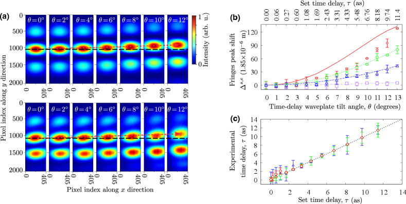
with , where and are the pixel indices along - and - directions, respectively. The function returns the index where the maximum value of is found. The reason why we sum over pixels is that tilting the time-delay waveplate around - axis inevitably leads to horizontal shifts due to refraction at the HWP (see Fig. 2(a)). Then, the classical Fisher information (CFI) for estimating is calculated as:
| (6) |
Calculations of the CFI assume only shot noise is present, and so serve as an upper bound on the precision of realistic measurements including technical noise. We present the theoretical calculation of in the Supplementary Material.
We first compare the CCD outcomes to the simulation when setting . Figure 2(a) illustrates that our experimental interference fringes closely match the simulations. Notably, the experimental CCD image exhibits asymmetry when measuring at , which can be attributed to a non-zero initial time delay arising from a slight misalignment of the two D-HWPs’ surfaces.
In this work, the WVA+interferometry sensitivity enhancement factor is defined by the slopes . Figure 2(b) demonstrates that selecting smaller post-selection angles results in more pronounced enhancements, characterized by steeper slopes. Our experimental data aligns closely with the simulations when and . For each delay and post-selection we make two separate sets of measurements. One is used to calibrate the relationship between delay and shift (shown in Fig. 2(b)), and the other is used to perform the delay estimation (shown in Fig. 2(c)).
In Fig. 3, we present the precision in the measurements by calculating for both the simulated and measured intensity distributions, as well as the actual SNR . Here, is the experimental variance in Fig. 2. The precision limit is defined as the Cramér-Rao bound, which is equal to the minimum variance achievable for any unbiased estimator. Numerically, this is equal to the inverse of the CFI. Since the actual estimation through calibration in Fig. 2(c) was influenced by technical noises in the system, the experimental SNR is expected to fall below the Cramér-Rao bound .
The experimentally determined values are generally lower than the simulated curves as shown in Fig. 3. We attribute this difference to imperfections in the measured diffraction pattern; the experimental probability distribution ) presented in the Supplementary Material is seen to have lower fringe visibility than is expected from the ideal measurement assumed in simulations. Fig. 3 indicates that some delays of the experimental SNR with setting lie close to the shot noise limit, demonstrating the ability of WVA+interferometry to approach shot-noise limited measurements.

Our experiment reveals two distinct error sources that impact precision. The systematic error originates from the precise control challenges associated with HWP rotations when preparing nearly orthogonal pre- and post-selected states (see Fig. 2(b) with ). However, Fig. 2(c) shows that the systematic error can be eliminated by calibrating the experimental data. The statistical errors resulting in the actual variance could come from environmental factors such as temperature and air pressure variations. Fig. 3 demonstrates that WVA+interferometry achieves a higher SNR (i.e. reduces the negative effect of technical noise) when choosing smaller post-selection angles.
In summary, we have proposed and experimentally demonstrated a way to integrate weak value amplification with precision interferometry. As an example, we amplified the delay between the slits of double-slit interferometer, which demonstrated a new efficient and cost-effective method for measuring few-attosecond time delays (see Fig. 2(b)) with precision approaching the shot noise limit and signal-to-noise ratios improved by up to three orders of magnitude (e.g., with post-selection setting , see Fig. 3). Our experiment is also the first measurement of this precision to use narrowband light for WVA, enabling a new class of WVA-based measurements of longitudinal phase.
Acknowledgements.
This study was supported by the NSFC (Grants No. 42327803 and No. 42220104002), the Canada Research Chairs Program, and the Natural Sciences and Engineering Research Council. J.H.H. acknowledges support from the CSC. A.C.D. acknowledges support from the EPSRC, Impact Acceleration Account (Grant No. EP/R511705/1).References
- Eberle et al. (2010) T. Eberle, S. Steinlechner, J. Bauchrowitz, V. Händchen, H. Vahlbruch, M. Mehmet, H. Müller-Ebhardt, and R. Schnabel, Phys. Rev. Lett. 104, 251102 (2010).
- Sorianello et al. (2018) V. Sorianello, M. Midrio, G. Contestabile, I. Asselberghs, J. V. Campenhout, C. Huyghebaert, I. Goykhman, A. K. Ott, A. C. Ferrari, and M. Romagnoli, Nature Photonics 12, 40 (2018).
- Abbott et al. (2016) B. P. Abbott et al. (LIGO Scientific Collaboration and Virgo Collaboration), Phys. Rev. Lett. 116, 061102 (2016).
- Nabekawa et al. (2009) Y. Nabekawa, T. Shimizu, Y. Furukawa, E. J. Takahashi, and K. Midorikawa, Phys. Rev. Lett. 102, 213904 (2009).
- Chen et al. (2021) X. Chen, M. E. Kandel, and G. Popescu, Adv. Opt. Photon. 13, 353 (2021).
- Pang et al. (2014) S. Pang, J. Dressel, and T. A. Brun, Phys. Rev. Lett. 113, 030401 (2014).
- Aharonov et al. (1988) Y. Aharonov, D. Z. Albert, and L. Vaidman, Phys. Rev. Lett. 60, 1351 (1988).
- Dressel et al. (2014) J. Dressel, M. Malik, F. M. Miatto, A. N. Jordan, and R. W. Boyd, Rev. Mod. Phys. 86, 307 (2014).
- Brunner and Simon (2010) N. Brunner and C. Simon, Phys. Rev. Lett. 105, 010405 (2010).
- Strübi and Bruder (2013) G. Strübi and C. Bruder, Phys. Rev. Lett. 110, 083605 (2013).
- Xu et al. (2013) X.-Y. Xu, Y. Kedem, K. Sun, L. Vaidman, C.-F. Li, and G.-C. Guo, Phys. Rev. Lett. 111, 033604 (2013).
- Pang and Brun (2015) S. Pang and T. A. Brun, Phys. Rev. Lett. 115, 120401 (2015).
- Xu et al. (2020) L. Xu, Z. Liu, A. Datta, G. C. Knee, J. S. Lundeen, Y. Q. Lu, and L. Zhang, Phys. Rev. Lett. 125, 080501 (2020).
- Krafczyk et al. (2021) C. Krafczyk, A. N. Jordan, M. E. Goggin, and P. G. Kwiat, Phys. Rev. Lett. 126, 220801 (2021).
- Harris et al. (2017) J. Harris, R. W. Boyd, and J. S. Lundeen, Phys. Rev. Lett. 118, 070802 (2017).
Enhancing interferometry using weak value amplification with real weak values: Supplementary Material
Appendix A Simulation and experimental probability distributions
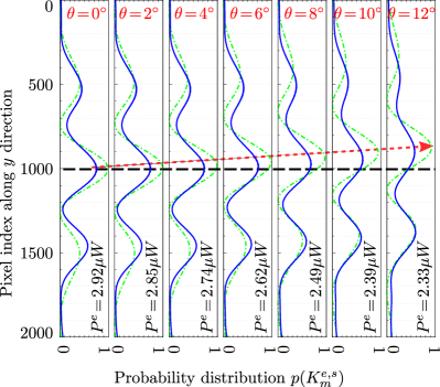
We display both the expectations and the experimental probability distributions along the direction with in Fig. 4. We use a sub-array of pixels in the - and - directions, respectively. It is evident that the shape of these fringes remains consistent, while the entire interference fringes shift with increasing time delay.
Appendix B Theoretical classical Fisher information calculation
The theoretical classical Fisher information (CFI) for estimating is calculated as:
| (7) |
Where represents the theoretical CCD outcomes. Drawing inspiration from investigations in the context of imperfect CCDs Harris et al. (2017); Xu et al. (2020), our simulation begins with the calculation of the theoretical distribution , which represents the expected average number of photons received by the CCD. Taking into account the proportionality between and , the distribution equals to the distribution . The total average photon number of the coherent beam is a fundamental parameter in our simulation, and it is determined by summing all photons at each pixel. For obtaining the simulation input, we maintain by measuring the optical average power before reaching the CCD. To achieve this congruence, we employ the relationship , where represents the exposure time, and each photon at 632.992 nm carries an energy of . The exposure time is set at = 2.0 ms, 1.0 ms, and 0.3 ms for , , and , respectively. The optical power detected before the PBS for post-selection is 2.0 mW. The average power with different and various are recorded for the simulation input. We also conduct a baseline measurement with , 3.0 and = 0.3 ms, representing the traditional interferometer without WVA enhancement. For a coherent beam, the exact number of the photoelectrons detected by the CCD follows a Poisson distribution
| (8) |
This Poisson process generates shot noise, which characterizes the fluctuations in the number of photons detected by CCD due to their independent occurrence. In simulation, we focus solely on the shot noise, disregarding other forms of electrical noise and ensuring avoidance of CCD saturation. Thus, we mathematically establish a conditional probability distribution = 1, linking with . Finally, the CCD outcomes closely approximate and are obtained through the Monte Carlo simulation of the Poisson process.