Enhancing Deep Traffic Forecasting Models with Dynamic Regression

Here, we review some signature frameworks for DL-based spatiotemporal traffic forecasting models. Starting from the DCRNN framework (Li et al. 2018), modern deep learning models are generally featured with a combination of different neural networks to process the spatial and temporal dependencies in traffic data. For example, DCRNN uses a diffusion convolution operation to model the spatial dependency. The convolution process is integrated into Gated Recurrent Units (GRUs) for modeling temporal dependency. The STGCN framework (Yu, Yin, and Zhu 2018) uses Graph Convolutional Networks (GCNs) to extract spatial correlations and Convolutional Neural Networks (CNNs) to extract temporal correlations. GCNs have the advantage of incorporating graph structure into the spatial modeling process. CNNs can reduce the training time through parallel computing since it avoids the recurrent process in Recurrent Neural Networks (RNNs). Building on STGCN, the ASTGCN framework (Guo et al. 2019) integrates a spatiotemporal attention mechanism to pre-process the traffic data before being fed to the convolutional layers. Both STGCN and ASTGCN use a pre-calibrated adjacency matrix that cannot be jointly learned with the model. The Graph WaveNet framework (Wu et al. 2019) uses an adaptive adjacency matrix to learn the graph structure. The entries in the adjacency matrix are treated as trainable parameters in the optimization. Dilated causal convolution is used as Temporal Convolutional Networks (TCNs) to model temporal dependency and GCNs are used to model spatial dependency. Prior GCN-based architectures process spatial information and temporal information separately. Song et al. proposed the STSGCN framework (Song et al. 2020) to learn spatial and temporal information simultaneously by connecting individual spatial graphs of adjacent time steps into one graph. STSGCN has shown superior performance to the previous GCN-based frameworks. Other SOTA models include GMAN (Zheng et al. 2020), N-BEATS (Oreshkin et al. 2020), and FC-GAGA (Oreshkin et al. 2021), to name a few.

Autocorrelated residuals in time series data have been extensively studied in econometrics, utilizing models with exact forms (Durbin and Watson 1950; Ljung and Box 1978; Breusch 1978; Godfrey 1978; Cochrane and Orcutt 1949; Prais and Winsten 1954; Beach and MacKinnon 1978). As DL models advance rapidly, the matter of how to learn and adapt the residual process has garnered notable attention in recent research. Two primary statistical approaches exist for modeling the residual process: (i) capturing autocorrelation, and (ii) learning concurrent correlation in independent errors.

To address autocorrelation, Sun, Lang, and Boning (2021) proposed a reparametrization strategy for the input and output of a neural network used in time series forecasting. This reparametrization inherently employs a first-order residual AR process through a linear regression framework. The method effectively enhances performance for various DL-based one-step-ahead forecasting models across a diverse range of time series datasets, enabling joint parameter optimization of both base and residual regressors. Additionally, Kim et al. (2022) introduced a lightweight DL module designed to calibrate residual autocorrelation within predictions from pre-trained traffic forecasting models. This calibration module employs recent observed residuals and predictions to anticipate future residuals, ultimately enhancing the performance of numerous traffic forecasting models, especially on traffic speed datasets.

Regarding learning concurrent correlation, Jia and Benson (2020) emphasized that assuming independence in residuals of a node regression problem is unwarranted. They advocated modeling concurrent correlation using a multivariate Gaussian distribution. This method, termed residual propagation in Graph Neural Networks (GNNs), adjusts predictions of unknown nodes based on known node labels. Similarly, Huang et al. (2021) introduced a correct-and-smooth approach, serving as a post-processing scheme to rectify correlated residuals in GNNs, focusing on a classification task. Additionally, Choi et al. (2022) proposed a dynamic mixture of matrix normal Gaussian as a regularization technique to address concurrent spatiotemporal correlation within residuals.

Traffic forecasting entails a multivariate sequence-to-sequence (Seq2Seq) framework entwined with strong seasonality, rendering direct applicability challenging. The primary obstacle lies in the residual process, which transforms into an $N\times Q$ matrix-variate time series, characterized by conspicuous temporal dynamics and a structured error covariance. The cohesive learning of this process and the base DL model constitutes a pivotal challenge.

Our work differs from Sun, Lang, and Boning (2021) and Kim et al. (2022) in several important ways. Firstly, we extend the scope of Sun, Lang, and Boning (2021) to encompass multivariate Seq2Seq forecasting, while also bypassing the need for input and output reparametrization. Secondly, our approach allows for the concurrent optimization of both the residual regression module and the base model, in contrast to the post-hoc adjustment presented by Kim et al. (2022). Lastly, we investigate the presence of seasonal autocorrelation, a substantial element in traffic forecasting, setting our work apart from the aforementioned studies.

A traffic network can be defined as a directed graph $\mathcal{G}=\left(\mathcal{V},\mathcal{E},\mathbf{W}\right)$, where $\mathcal{V}$ with $|\mathcal{V}|=N$ is a set of nodes representing traffic sensors; $\mathcal{E}$ is a set of links connecting these nodes; $\mathbf{W}\in\mathbb{R}^{N\times N}$ is a weighted adjacency matrix characterizing the proximity of nodes. Denote by $\boldsymbol{z}_{t}\in\mathbb{R}^{N}$ the vector of observed traffic states at time $t$. The traffic forecasting problem aims to learn a function that maps data from $P$ past steps to the prediction of $Q$ future steps.

Denote by $\boldsymbol{X}_{t}=\left[\boldsymbol{z}_{t-P+1},\dots,\boldsymbol{z}_{t}\right]\in\mathbb{R}^{N\times P}$ and $\boldsymbol{Y}_{t}=\left[\boldsymbol{z}_{t+1},\dots,\boldsymbol{z}_{t+Q}\right]\in\mathbb{R}^{N\times Q}$, we have

$${\boldsymbol{Y}}_{t}=f_{\theta}(\boldsymbol{X}_{t},\mathbf{W})+\boldsymbol{R}_{t},$$

(1)

where $f_{\theta}(\boldsymbol{X}_{t},\mathbf{W})$ is a Seq2Seq DL model that generates the predicted mean and $\boldsymbol{R}_{t}\in\mathbb{R}^{N\times Q}$ is a zero-mean residual process. In many cases, $f_{\theta}(\cdot)$ is trained with MSE as the loss function:

$$\mathcal{L}=\sum_{t}\|\boldsymbol{R}_{t}\|_{F}^{2}=\sum_{t}\|\boldsymbol{Y}_{t}-f_{\theta}(\boldsymbol{X}_{t},\mathbf{W})\|_{F}^{2}.$$

(2)

This loss function simply assumes: (i) $\boldsymbol{R}_{t}$ is temporally independent, i.e., there is no correlation between $\boldsymbol{R}_{s}$ and $\boldsymbol{R}_{t}$ when $s\neq t$; and (ii) entries in $\boldsymbol{R}_{t}$ follow an isotropic Gaussian with no concurrent correlations, i.e., $\boldsymbol{\eta}_{t}=\operatorname{vec}(\boldsymbol{R}_{t})\sim\mathcal{N}(\mathbf{0},\sigma^{2}\mathbf{I}_{NQ})$. Likewise, using MAE as the loss function corresponds to assuming entries in $\boldsymbol{R}_{t}$ follow a Laplacian distribution.

Following the idea of dynamic regression (Hyndman and Athanasopoulos 2018), we assume that the relationship between the input $\boldsymbol{X}_{t}$ and the output $\boldsymbol{Y}_{t}$ has not been fully captured by $f_{\theta}(\cdot)$, and the unexplained residual $\boldsymbol{R}_{t}$ is governed by a temporal process. For example, for a one-step-ahead prediction model (i.e., $\boldsymbol{\eta}_{t}=\boldsymbol{R}_{t}$ as $Q=1$), it is straightforward to model $\boldsymbol{\eta}_{t}$ using a $p$-th order vector autoregressive model:

$$\boldsymbol{\eta}_{t}=\boldsymbol{C}_{1}\boldsymbol{\eta}_{t-1}+\ldots+\boldsymbol{C}_{p}\boldsymbol{\eta}_{t-p}+\boldsymbol{\epsilon}_{t},$$

(3)

where $\boldsymbol{C}_{l}\in\mathbb{R}^{N\times N}$ ($l=1,\ldots,p$) are the regression coefficient, and $\boldsymbol{\epsilon}_{t}\sim\mathcal{N}\left(\mathbf{0},\boldsymbol{\Sigma}\right)$ is an independent white-noise process.

However, for a Seq2Seq model with $Q>1$, the $N\times Q$ residual $\boldsymbol{R}_{t}$ at time $t$ cannot be directly modeled using Eq. (3), as the residuals, $\{\boldsymbol{R}_{t-l}\,|\,l=1,\ldots,Q-1\}$, will not be entirely accessible due to overlapping. To address this issue, we instead try to model the relation between $\boldsymbol{R}_{t}$ and those lagged residuals that are accessible, i.e., $\boldsymbol{R}_{t-\Delta_{l}}$ for $l=1,\ldots,p$ as long as $\Delta_{l}\geq Q$. Therefore, we have the model for the vector $\boldsymbol{\eta}_{t}$ as:

$$\boldsymbol{\eta}_{t}=\boldsymbol{C}_{1}\boldsymbol{\eta}_{t-\Delta_{1}}+\ldots+\boldsymbol{C}_{p}\boldsymbol{\eta}_{t-\Delta_{p}}+\boldsymbol{\epsilon}_{t},$$

(4)

where $\boldsymbol{C}_{l}\in\mathbb{R}^{NQ\times NQ}$ and the size of the white-noise covariance matrix $\boldsymbol{\Sigma}$ is also of size $NQ\times NQ$. As traffic data often shows strong day-to-day and week-to-week similarity, for simplicity we only introduce a single lagged residual component $\boldsymbol{R}_{t-\Delta}$, where $\Delta$ is a predetermined seasonal lag (e.g., one day or one week) showcasing pronounced correlations with the present time.

However, a notable limitation of the aforementioned formulation is the introduction of an excessive number of parameters within $\boldsymbol{C}$ and $\boldsymbol{\Sigma}$. For improved scalability of this approach, we assume the $\boldsymbol{R}_{t}$ follows a bi-linear autoregressive model (Chen, Xiao, and Yang 2021; Hsu, Huang, and Tsay 2021):

$$\boldsymbol{R}_{t}=\boldsymbol{A}\boldsymbol{R}_{t-\Delta}\boldsymbol{B}+\boldsymbol{E}_{t},$$

(5)

where $\boldsymbol{A}\in\mathbb{R}^{N\times N}$ and $\boldsymbol{B}\in\mathbb{R}^{Q\times Q}$ are regression coefficients, and $\boldsymbol{E}_{t}$ follows an independent matrix white-noise process. The vectorized version of Eq. (5) becomes

$$\boldsymbol{\eta}_{t}=(\boldsymbol{B}^{\top}\otimes\boldsymbol{A})\boldsymbol{\eta}_{t-\Delta}+\boldsymbol{\epsilon}_{t},$$

(6)

and we can see that the bi-linear formulation is equivalent to imposing a Kronecker product structure on the coefficient matrix $\boldsymbol{C}=\boldsymbol{B}^{\top}\otimes\boldsymbol{A}$ in Eq. (4), leading to a significant reduction in the parameters. Combining Eqs. (1) and (5), we can construct an improved loss function, such as MAE, on $\boldsymbol{E}_{t}$ instead of $\boldsymbol{R}_{t}$:

$$\boldsymbol{E}_{t}=\boldsymbol{Y}_{t}-f_{\theta}(\boldsymbol{X}_{t})-\boldsymbol{A}\left(\boldsymbol{Y}_{t-\Delta}-f_{\theta}(\boldsymbol{X}_{t-\Delta})\right)\boldsymbol{B},$$

(7)

$$\mathcal{L}_{\text{mae}}=\sum_{t}\|\boldsymbol{E}_{t}\|_{1},$$

(8)

where $\boldsymbol{A}$ and $\boldsymbol{B}$, as trainable parameters, can be jointly updated with the base model $f_{\theta}(\cdot)$. When $\boldsymbol{R}_{t}$ and $\boldsymbol{R}_{t-\Delta}$ have no relations (e.g., when $\boldsymbol{A}=\boldsymbol{0}$), $\mathcal{L}_{\text{mae}}$ collapse to the default MAE loss used in existing DL models. If both $\boldsymbol{A}$ and $\boldsymbol{B}$ are identity matrices, the model corresponds to assuming the residual process follows a seasonal random walk. To promote sparsity in $\boldsymbol{A}$ and $\boldsymbol{B}$, we also introduce an $l1$ regularization term into the loss function:

$$\mathcal{L}_{\text{res}}=\frac{1}{N^{2}}\|\boldsymbol{A}\|_{1}+\frac{1}{Q^{2}}\|\boldsymbol{B}\|_{1}.$$

(9)

Once $f_{\theta}(\cdot)$ and coefficients $\boldsymbol{A}$ and $\boldsymbol{B}$ are learned, prediction at time $t$ can be made by:

$$\hat{\boldsymbol{Y}}_{t}=f_{\theta}(\boldsymbol{X}_{t})+\boldsymbol{A}\left(\boldsymbol{Y}_{t-\Delta}-f_{\theta}(\boldsymbol{X}_{t-\Delta})\right)\boldsymbol{B}.$$

(10)

We next try to consider the concurrent spatiotemporal correlation among entries in the white noise $\boldsymbol{E}_{t}$ through learning its covariance matrix $\boldsymbol{\Sigma}$. The key challenge here is the large size (i.e., $NQ\times NQ$) of $\boldsymbol{\Sigma}$. For model scalability, we follow Choi et al. (2022) and assume $\boldsymbol{E}_{t}$ to follow a zero-mean matrix normal distribution $\boldsymbol{E}_{t}\sim\mathcal{MN}(\boldsymbol{0},\boldsymbol{\Sigma}_{N},\boldsymbol{\Sigma}_{Q})$ with

$\displaystyle p\left(\boldsymbol{E}_{t}\right)=\frac{\exp{\left(-\frac{1}{2}\operatorname{tr}\left(\boldsymbol{\Sigma}_{Q}^{-1}\boldsymbol{E}_{t}^{\top}\boldsymbol{\Sigma}_{N}^{-1}\boldsymbol{E}_{t}\right)\right)}}{(2\pi)^{\frac{NQ}{2}}|\boldsymbol{\Sigma}_{Q}|^{\frac{N}{2}}|\boldsymbol{\Sigma}_{N}|^{\frac{Q}{2}}},$

(11)

where $\boldsymbol{\Sigma}_{N}$ and $\boldsymbol{\Sigma}_{Q}$ are covariance matrices of the matrix normal distribution capturing the correlation across forecasting steps and spatial locations. The negative log-likelihood of this distribution is included in the loss function to facilitate joint optimization:

	$\displaystyle\mathcal{L}_{\text{nll}}$	$\displaystyle=-\log p(\boldsymbol{E}_{t}\,|\,\boldsymbol{0},\boldsymbol{\Sigma}_{N},\boldsymbol{\Sigma}_{Q})$		(12)
		$\displaystyle=\frac{NQ}{2}\log(2\pi)+\frac{Q}{2}\log|\boldsymbol{\Sigma}_{N}|+\frac{N}{2}\log|\boldsymbol{\Sigma}_{Q}|$
		$\displaystyle+\frac{1}{2}\operatorname{tr}\left(\boldsymbol{\Sigma}_{Q}^{-1}\boldsymbol{E}_{t}^{\top}\boldsymbol{\Sigma}_{N}^{-1}\boldsymbol{E}_{t}\right).$

As we have to calculate the inverse and determinant of $\boldsymbol{\Sigma}_{N}$, $\boldsymbol{\Sigma}_{Q}$, we parameterize the precision matrix (i.e., the inverse of the covariance matrix) directly to circumvent numerical problems. Another benefit of parameterizing precision matrices lies in their ability to model conditional independence between two variables, based on the observations of other variables. This modeling introduces zero elements in precision matrices when two variables are conditionally independent, resulting in significantly sparse matrices that augment the scalability of our approach. The tangible interpretation of a precision matrix signifies the lack of an edge connecting two nodes in a graph when they are conditionally independent (Adametz and Roth 2014). This characteristic holds special importance in the realm of traffic forecasting, where each traffic sensor is typically connected to a limited number of other sensors.

In this paper, we consider the Cholesky decomposition of the precision matrix as trainable parameters following Choi et al. (2022):

$$\begin{split}&\boldsymbol{\Sigma}_{N}^{-1}=\boldsymbol{\Lambda}_{N},\ \ \boldsymbol{\Sigma}_{Q}^{-1}=\boldsymbol{\Lambda}_{Q},\\ &\boldsymbol{\Lambda}_{N}=\boldsymbol{L}_{N}\boldsymbol{L}_{N}^{\top},\ \ \boldsymbol{\Lambda}_{Q}=\boldsymbol{L}_{Q}\boldsymbol{L}_{Q}^{\top},\end{split}$$

(13)

where $\boldsymbol{L}_{N}\in\mathbb{R}^{N\times N}$ and $\boldsymbol{L}_{Q}\in\mathbb{R}^{Q\times Q}$ are lower-triangular Cholesky factors (as trainable parameters) that can be jointly optimized with other model parameters. The determinant can be conveniently calculated by summing the logarithm of diagonal entries of the lower triangular Cholesky factors:

$$\begin{split}\log|\boldsymbol{\Sigma}_{N}|&=-\log|\boldsymbol{\Lambda}_{N}|=-2\sum_{n=1}^{N}\log[\boldsymbol{L}_{N}]_{n,n},\\ \log|\boldsymbol{\Sigma}_{Q}|&=-\log|\boldsymbol{\Lambda}_{Q}|=-2\sum_{q=1}^{Q}\log[\boldsymbol{L}_{Q}]_{q,q}.\\ \end{split}$$

(14)

In addition, the trace can be simplified into

	$\displaystyle\operatorname{tr}\left(\boldsymbol{\Lambda}_{Q}\boldsymbol{E}_{t}^{\top}\boldsymbol{\Lambda}_{N}\boldsymbol{E}_{t}\right)$	$\displaystyle=\operatorname{tr}\left(\boldsymbol{L}_{Q}\boldsymbol{L}_{Q}^{\top}\boldsymbol{E}_{t}^{\top}\boldsymbol{L}_{N}\boldsymbol{L}_{N}^{\top}\boldsymbol{E}_{t}\right)$		(15)
		$\displaystyle=\operatorname{tr}\left(\boldsymbol{L}_{N}^{\top}\boldsymbol{E}_{t}\boldsymbol{L}_{Q}\boldsymbol{L}_{Q}^{\top}\boldsymbol{E}_{t}^{\top}\boldsymbol{L}_{N}\right)$
		$\displaystyle=\operatorname{tr}\left(\boldsymbol{K}_{t}\boldsymbol{K}_{t}^{\top}\right)=\|\boldsymbol{K}_{t}\|_{F}^{2},$

where $\boldsymbol{K}_{t}=\boldsymbol{L}_{N}^{\top}\boldsymbol{E}_{t}\boldsymbol{L}_{Q}$. Substitute Eq. (14) and Eq. (15) into Eq. (12), we obtain a probabilistic loss function to learn the correlation structure in $\boldsymbol{E}_{t}$:

$$\mathcal{L}_{\text{nll}}=\frac{1}{2}\|\boldsymbol{K}_{t}\|_{F}^{2}-Q\sum_{n=1}^{N}\log[\boldsymbol{L}_{N}]_{n,n}-N\sum_{q=1}^{Q}\log[\boldsymbol{L}_{Q}]_{q,q}.$$

(16)

As the covariance matrix determines the concurrent spatiotemporal correlations in $\boldsymbol{E}_{t}$, we posit that it will not only improve model accuracy but also provide better uncertainty quantification when performing probabilistic forecasting.

Aligned with the chosen datasets for method validation, we assess our approach using the following models as the base model $f_{\theta}(\cdot)$.

• •

  STGCN (Yu, Yin, and Zhu 2018): Spatiotemporal graph convolutional network, which uses ChebNet to process spatial correlation and CNNs to process temporal correlation.

• •

  ASTGCN (Guo et al. 2019): Attention-based spatiotemporal graph convolutional network, which attaches spatial and temporal attention mechanisms to STGCN for learning dynamic spatial-temporal correlations of traffic data.

• •

  STSGCN (Song et al. 2020): Spatial-temporal synchronous graph convolutional network that captures spatial-temporal correlations over the time axis.

• •

  Graph WaveNet (Wu et al. 2019): A spatiotemporal forecasting model that combines dilated 1D convolution for modeling temporal dynamics and graph convolution for modeling spatial dynamics.

Our experimental setup involved a computer environment featuring an Intel(R) Xeon(R) CPU E5-2698 v4 @ 2.20GHz and four NVIDIA Tesla V100 GPUs. Baseline models were implemented using either the original source code or their PyTorch versions. All models were configured to employ 12 historical observation steps ($P=12$) for predicting 12 future steps ($Q=12$). During training, the Adam optimizer was utilized with an initial learning rate of 0.001 and a weight decay of 0.0001. To prevent overfitting, early stopping was employed when the validation loss showed consistent increase over 30 epochs. All reported outcomes are based on the average of evaluation metrics derived from three independent runs.

For the residual AR process, we need to determine the lag length $\Delta$ and the initialization of the regression coefficients $\boldsymbol{A}$ and $\boldsymbol{B}$. Since traffic data is featured with strong local correlation and seasonality, we mainly consider the correlation between the current residual and its 1) most recent available predecessor ($\Delta=Q$); 2) counterpart one day apart ($\Delta=\text{1 day}$); and 3) counterpart one week apart ($\Delta=\text{1 week}$). The inclusion of seasonal residual correlation is novel to prior works (Sun, Lang, and Boning 2021; Kim et al. 2022). Regarding the initialization of $\boldsymbol{A}$ and $\boldsymbol{B}$, we attempt three different settings: 1) random. $\boldsymbol{A}$ and $\boldsymbol{B}$ consist of random numbers sampled from a normal distribution with mean 0 and variance 1; 2) zeros. $\boldsymbol{A}$ and $\boldsymbol{B}$ are zero matrices; 3) diagonal. $\boldsymbol{A}$ and $\boldsymbol{B}$ are diagonal matrices. The initial values of parameters in these settings are scaled down to very small numbers so that the model is nearly equivalent to the original model at the beginning of the training stage. Based on the preliminary observation of autocorrelation matrices, we used $\Delta=Q$ for PEMSD7 (M), $\Delta=\text{1 day}$ for PEMS03, and $\Delta=\text{1 week}$ for PEMS08. For the initialization, we chose “random” and “zeros” for STGCN and Graph WaveNet on PEMSD7 (M), “diagonal” for PEMS03, and “random” for PEMS08. For the parameters of the matrix normal distribution in section Spatiotemporal Covariance Structure for the Matrix White Noise, the matrices $\boldsymbol{L}_{N}$ and $\boldsymbol{L}_{Q}$ consist of random numbers sampled from a normal distribution with mean 0 and variance 1. The Softplus function is applied to enforce positive diagonals of $\boldsymbol{L}_{Q}$ and $\boldsymbol{L}_{N}$.

The final loss function is composed of three parts:

$$\mathcal{L}=\mathcal{L}_{\text{mae}}+\omega\mathcal{L}_{\text{res}}+\rho\mathcal{L}_{\text{nll}},$$

(17)

where $\mathcal{L}_{\text{mae}}$ and $\mathcal{L}_{\text{res}}$ are the MAE loss built on Eq. (8) and the $l1$ regularization in Eq. (9), respectively, $\mathcal{L}_{\text{nll}}$ is the probabilistic loss term in Eq. (16), and $\omega$ and $\rho$ are weight parameters. We set $\omega=1$, and use $\rho=0.001$ for PEMSD7 (M) and PEMS03, $\rho=0.0001$ for PEMS08. The evaluation metrics are MAE and RMSE. Missing values are excluded from both training and testing.

In comparison to the base model, the proposed method introduces four additional learnable parameters, i.e., $\boldsymbol{A}\in\mathbb{R}^{N\times N}$, $\boldsymbol{B}\in\mathbb{R}^{Q\times Q}$, and two lower-triangular Cholesky factors $\boldsymbol{L}_{N}$ and $\boldsymbol{L}_{Q}$. Nevertheless, the size of additional parameters is almost negligible compared to the overall size of the base model.

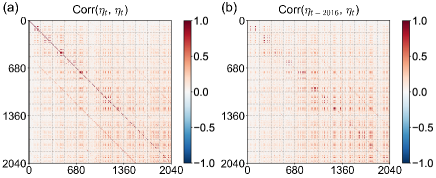
We begin by demonstrating both the autocorrelation and the concurrent spatiotemporal correlations of the residuals from an original traffic forecasting model. We calculate two types of correlation: $\operatorname{Corr}(\boldsymbol{\eta}_{t},\boldsymbol{\eta}_{t})$ and $\operatorname{Corr}(\boldsymbol{\eta}_{t-\Delta},\boldsymbol{\eta}_{t})$. $\operatorname{Corr}(\boldsymbol{\eta}_{t},\boldsymbol{\eta}_{t})$ is the concurrent spatiotemporal correlation of the variables in $\boldsymbol{\eta}_{t}$, while $\operatorname{Corr}(\boldsymbol{\eta}_{t-\Delta},\boldsymbol{\eta}_{t})$ is the autocorrelation at lag $\Delta$. Ideally, if the residuals are independently sampled from an isotropic distribution, $\operatorname{Corr}(\boldsymbol{\eta}_{t},\boldsymbol{\eta}_{t})$ should be an identity matrix and $\operatorname{Corr}(\boldsymbol{\eta}_{t-\Delta},\boldsymbol{\eta}_{t})$ should be a zero matrix. In Figure 2, we present the residual correlation matrices of PEMS08 using the results from Graph WaveNet. We can observe that $\operatorname{Corr}(\boldsymbol{\eta}_{t},\boldsymbol{\eta}_{t})$ is not diagonal, suggesting there exists spatial and across-step correlations in the residuals. In terms of $\operatorname{Corr}(\boldsymbol{\eta}_{t-\Delta},\boldsymbol{\eta}_{t})$, we examine different values including $\Delta=12$ (1 hour), $\Delta=288$ (1 day), and $\Delta=2016$ (1 week). Interestingly, we find that $\Delta=2016$ provides the strongest autocorrelation patterns, while correlations with $\Delta=12$ and $\Delta=288$ are weak. We believe this is mainly due to the fact that traffic flow is heavily determined by travel demand, which often exhibits prominent weekly periodicity. Therefore, we choose $\Delta=2016$ for the residual AR process for PEMS08.

Table 2 presents a comprehensive summary of our approach’s performance across diverse DL models and datasets, spanning prediction horizons of 1-step, 3-step, 6-step, and 12-step ahead. Notably, our method consistently yields superior outcomes across nearly all scenarios. Graph WaveNet’s exceptional performance is particularly noteworthy, primarily stemming from its implementation of the adaptive adjacency matrix. Upon adopting our approach, Graph WaveNet demonstrates substantial additional enhancement, even in scenarios where the original models already excel, such as the 1-step ahead prediction. A case in point is the 1-step MAE of Graph WaveNet on PEMS08, which decreases from 12.81 to 11.66, signifying the presence of explainable factors eluding the original model’s grasp.

Figure 3 visually illustrates the marked reduction in both concurrent spatiotemporal correlation and autocorrelation, when compared to Figure 2. Notably, our approach exhibits amplified enhancement for models manifesting stronger residual correlations, such as STSGCN and ASTGCN, with particularly pronounced benefits observed for the 12-step ahead prediction. For example, the 12-step MAE of ASTGCN on PEMS08 decreases from 21.57 to 17.99. These diverse yet discernible improvements underscore that our method’s efficacy is contingent upon the degree of autocorrelation inherent in the original models’ residuals, alongside the suitability of the matrix normal distribution assumption in characterizing errors.

References

- Adametz and Roth (2014) Adametz, D.; and Roth, V. 2014. Distance-based network recovery under feature correlation. Advances in Neural Information Processing Systems, 27.
- Beach and MacKinnon (1978) Beach, C. M.; and MacKinnon, J. G. 1978. A maximum likelihood procedure for regression with autocorrelated errors. Econometrica: journal of the Econometric Society, 51–58.
- Breusch (1978) Breusch, T. S. 1978. Testing for autocorrelation in dynamic linear models. Australian Economic Papers, 17(31): 334–355.
- Chen, Xiao, and Yang (2021) Chen, R.; Xiao, H.; and Yang, D. 2021. Autoregressive models for matrix-valued time series. Journal of Econometrics, 222(1): 539–560.
- Cheng, Trépanier, and Sun (2021) Cheng, Z.; Trépanier, M.; and Sun, L. 2021. Incorporating travel behavior regularity into passenger flow forecasting. Transportation Research Part C: Emerging Technologies, 128: 103200.
- Choi et al. (2022) Choi, S.; Saunier, N.; Zheng, V. Z.; Trepanier, M.; and Sun, L. 2022. Scalable Dynamic Mixture Model with Full Covariance for Probabilistic Traffic Forecasting. arXiv preprint arXiv:2212.06653.
- Cochrane and Orcutt (1949) Cochrane, D.; and Orcutt, G. H. 1949. Application of least squares regression to relationships containing auto-correlated error terms. Journal of the American Statistical Association, 44(245): 32–61.
- Durbin and Watson (1950) Durbin, J.; and Watson, G. S. 1950. Testing for serial correlation in least squares regression: I. Biometrika, 37(3/4): 409–428.
- Godfrey (1978) Godfrey, L. G. 1978. Testing against general autoregressive and moving average error models when the regressors include lagged dependent variables. Econometrica: Journal of the Econometric Society, 1293–1301.
- Guo et al. (2019) Guo, S.; Lin, Y.; Feng, N.; Song, C.; and Wan, H. 2019. Attention based spatial-temporal graph convolutional networks for traffic flow forecasting. In AAAI Conference on Artificial Intelligence, volume 33, 922–929.
- Hsu, Huang, and Tsay (2021) Hsu, N.-J.; Huang, H.-C.; and Tsay, R. S. 2021. Matrix autoregressive spatio-temporal models. Journal of Computational and Graphical Statistics, 30(4): 1143–1155.
- Huang et al. (2021) Huang, Q.; He, H.; Singh, A.; Lim, S.-N.; and Benson, A. R. 2021. Combining label propagation and simple models out-performs graph neural networks. In International Conference on Learning Representations.
- Hyndman and Athanasopoulos (2018) Hyndman, R. J.; and Athanasopoulos, G. 2018. Forecasting: Principles and Practice. OTexts.
- Jia and Benson (2020) Jia, J.; and Benson, A. R. 2020. Residual correlation in graph neural network regression. In Proceedings of the 26th ACM SIGKDD International Conference on Knowledge Discovery & Data Mining, 588–598.
- Kim et al. (2022) Kim, D.; Cho, Y.; Kim, D.; Park, C.; and Choo, J. 2022. Residual Correction in Real-Time Traffic Forecasting. In Proceedings of the 31st ACM International Conference on Information & Knowledge Management, 962–971.
- Li et al. (2018) Li, Y.; Yu, R.; Shahabi, C.; and Liu, Y. 2018. Diffusion convolutional recurrent neural network: Data-driven traffic forecasting. In International Conference on Learning Representations.
- Ljung and Box (1978) Ljung, G. M.; and Box, G. E. 1978. On a measure of lack of fit in time series models. Biometrika, 65(2): 297–303.
- Oreshkin et al. (2021) Oreshkin, B. N.; Amini, A.; Coyle, L.; and Coates, M. J. 2021. FC-GAGA: Fully Connected Gated Graph Architecture for spatio-temporal traffic forecasting. In AAAI Conference on Artificial Intelligence.
- Oreshkin et al. (2020) Oreshkin, B. N.; Carpov, D.; Chapados, N.; and Bengio, Y. 2020. N-BEATS: Neural basis expansion analysis for interpretable time series forecasting. In International Conference on Learning Representations.
- Prais and Winsten (1954) Prais, S. J.; and Winsten, C. B. 1954. Trend estimators and serial correlation. Technical report, Cowles Commission discussion paper Chicago.
- Song et al. (2020) Song, C.; Lin, Y.; Guo, S.; and Wan, H. 2020. Spatial-temporal synchronous graph convolutional networks: A new framework for spatial-temporal network data forecasting. In AAAI Conference on Artificial Intelligence, volume 34, 914–921.
- Sun, Lang, and Boning (2021) Sun, F.-K.; Lang, C.; and Boning, D. 2021. Adjusting for autocorrelated errors in neural networks for time series. Advances in Neural Information Processing Systems, 34: 29806–29819.
- Vlahogianni, Karlaftis, and Golias (2014) Vlahogianni, E. I.; Karlaftis, M. G.; and Golias, J. C. 2014. Short-term traffic forecasting: Where we are and where we’re going. Transportation Research Part C: Emerging Technologies, 43: 3–19.
- Wu et al. (2019) Wu, Z.; Pan, S.; Long, G.; Jiang, J.; and Zhang, C. 2019. Graph wavenet for deep spatial-temporal graph modeling. In Proceedings of the 28th International Joint Conference on Artificial Intelligence, 1907–1913. AAAI Press.
- Yu, Yin, and Zhu (2018) Yu, B.; Yin, H.; and Zhu, Z. 2018. Spatio-temporal graph convolutional networks: a deep learning framework for traffic forecasting. In Proceedings of the 27th International Joint Conference on Artificial Intelligence, 3634–3640. AAAI Press.
- Zheng et al. (2020) Zheng, C.; Fan, X.; Wang, C.; and Qi, J. 2020. Gman: A graph multi-attention network for traffic prediction. In AAAI Conference on Artificial Intelligence, volume 34, 1234–1241.