Enhancement of spin-mixing conductance by - orbital hybridization in heavy metals
Abstract
In a magnetic multilayer, the spin transfer between localized magnetization dynamics and itinerant conduction spin arises from the interaction between a normal metal and an adjacent ferromagnetic layer. The spin-mixing conductance then governs the spin-transfer torques and spin pumping at the magnetic interface. Theoretical description of spin-mixing conductance at the magnetic interface often employs a single conduction-band model. However, there is orbital hybridization between conduction electron and localized electron of the heavy transition metal, in which the single conduction-band model is insufficient to describe the - orbital hybridization. In this work, using the generalized Anderson model, we estimate the spin-mixing conductance that arises from the - orbital hybridization. We find that the orbital hybridization increases the magnitude of the spin-mixing conductance.
I Introduction
The technological potential of magnetic devices based on transition metals for spin-current manipulation has pushed research forward in the spintronics area [1]. The basic structure of a magnetic device is a magnetic multilayer. In spin-based memory systems, the interaction between normal metal and ferromagnetic metal can cause the magnetization direction to change [2].
In a magnetic multilayer, magnetization dynamics can be induced by spin current via the spin-transfer torque effect [3]. When the non magnetic layer has a finite spin accumulation , which represents the difference of the spin-dependent electrochemical potential, the magnetization near the ferromagnetic interface experiences a torque due to spin transfer [4]
| (1) |
where is spin-mixing conductance. Reciprocally, in spin pumping, the spin current can be induced by magnetization dynamic m via the exchange interaction between magnetization and spin of the conduction electron [5]. An adiabatic precession of the magnetization pumps a spin current from the ferromagnet to the nonmagnetic layer with a polarization[6, 7, 8]
| (2) |
Both spin transfer torque and spin pumping effects are governed by the same , which has a complex value with a comparably small imaginary term [9].
Spin-mixing conductance was originally described using spin-dependent scattering theory [5]. The basic theoretical models of spin-mixing conductance utilizes a non-interacting electron model for the nonmagnetic metal [10, 11]. While this is certainly appropriate for free-electron-like metals, it is less so for heavy transition metals [12]. To accommodate the localized symmetry of the electron, a linear response theory description of spin-mixing conductance has been developed [11]. However, there are few theoretical studies exploring the spin-mixing conductance of heavy metals with interacting electron model [13]. Therefore, a better understanding of the spin-mixing conductance of heavy metals is required.
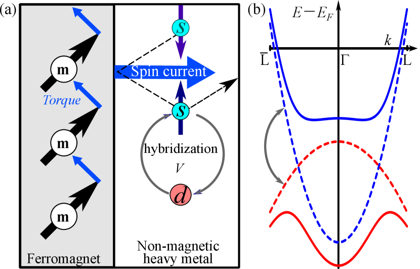
The theoretical description of spin-mixing conductance is often simplified in order to focus on a certain aspect or interaction that dominates a particular setup [14]. In the spin-pumping setup involving a heavy-metal system discussed in this article, we focus on the effect of electron-electron interaction at the nonmagnetic heavy metal layer. While the effect of electron interaction on spin-mixing conductance has been studied using Stoner model and phenomenological Hubbard parameter [15, 16, 17], a more realistic model of the heavy-metal system requires orbital hybridization [18], for example, the Anderson model [19]. In the Anderson model, a electron is treated as an impurity, with well-localized energy dispersion [20]. For describing a heavy metal, however, we need to consider a electron with a more generalized dispersion [21]. This article aims to theoretically estimate the electron-electron interaction correction factor due to the - orbital hybridization of a heavy metal as illustrated in Fig. 1.
In this article, we first analyze the linear response theory of spin density in heavy transition metal using Anderson model in Sec. II. In Sec. III we show that the orbital hybridization enhances of the interface of ferromagnet and heavy transition metal (Ta, W, Ir, Pt or Au). Lastly, we summarize our findings in Sec. IV.
II linear response theory in heavy transition metal
Near the magnetic interface, the exchange interaction between the localized magnetic moments m at the magnetic interface and the conduction spin can be written in the following Hamiltonian
| (3) |
where the exchange constant in the strong screening limit is [11, 4]. and are saturation magnetization and gyromagnetic ratio of the ferromagnetic insulator, respectively. is the density of states of the conduction electron at the Fermi level.
Using linear response theory, one can show the response of to m via spin susceptibility
| (4) |
where
| (5) |
Here is Heaviside step function. In an ,isotropic medium can be written in terms of and
| (6) |
where
Here and () are Pauli matrices. Since can be obtained by replacing and , it is convenient to discuss .
For a noninteracting simple metal with parabolic dispersion , in a small- limit is [11]
| (7) |
where is the low-temperature Fermi-Dirac distribution with wave vector k.
This single-band picture is appropriate for simple metals, such as light transition metals. Meanwhile, for heavy transition metal such as Au, W, Ta, and Pt, a localized -electron can mixed with the band, as illustrated in the band structure [see Fig. 1(b)]. The band structure can be obtained from density functional theory (DFT) software [22, 23] (see the appendix). Because of that, to determine the of heavy metal, we need to modify the single-band Hamiltonian with an appropriate Hamiltonian that accommodates the hybridization of and electron.
In the second quantization, the interactions in a heavy-metal system near the interface that is illustrated in Fig. 1 can be written with the following Hamiltonian based on the Anderson model [19, 20]
| (13) |
where is the hybridization parameter, is the creation (annihilation) operator of electron with wave vector k and spin and is the creation (annihilation) operator of the electron with spin . The second term corresponds to the - hybridization. Here is Pauli vectors. The energy dispersion of and electrons can be assumed to be parabolic
| (14) |
as illustrated in Fig. 4.
| Heavy metal | crystal | (Å) | path | band | Without spin-orbit coupling | With spin-orbit coupling | |||||||
| element | structure | (eV) | (eV) | (eV) | (eV) | ||||||||
| Au | fcc | 2.88 | L | 2.44 | 8.86 | 1.19 | 0.09 | 2.53 | 8.23 | 1.28 | 0.15 | ||
| 4.27 | 4.19 | 4.05 | 5.46 | ||||||||||
| W | bcc | 2.74 | N | 2.38 | 8.74 | 0.84 | 0.10 | 2.34 | 8.58 | 0.86 | 0.11 | ||
| 1.98 | 2.01 | 2.09 | 2.17 | ||||||||||
| Ta | bcc | 2.87 | N | 2.28 | 7.18 | 0.78 | 0.22 | 2.25 | 7.02 | 0.79 | 0.25 | ||
| 0.12 | 1.56 | -0.02 | 1.70 | ||||||||||
| Ir | fcc | 2.74 | L | 3.76 | 8.95 | 0.97 | 0.27 | 3.62 | 9.08 | 1.12 | 0.27 | ||
| 2.94 | 2.96 | 2.67 | 3.33 | ||||||||||
| Pt | fcc | 2.77 | L | 3.22 | 8.58 | 1.21 | 0.30 | 3.32 | 8.17 | 1.12 | 0.37 | ||
| 3.14 | 5.07 | 3.03 | 5.01 | ||||||||||
As illustrated in Fig. 1, the electron dominates the spin-mixing process at the interface. Therefore, we can define from the spin density of the electron
| (15) |
The susceptibility and its Fourier transform can be determined by evaluating its time derivation using the Heisenberg equation
| (16) |
Here is the unperturbed Hamiltonian in Eq. (13). Due to the hybridization of and orbitals, combinations of creation () and annihilation () operators appear when the commutations are evaluated. For convenience, we define
| (17) |
where
| (18) |
in the frequency domain can now be obtained from a matrix relation
| (31) |
Let us note that since susceptibility is a retarded response [8], has a negligibly small imaginary term as in Eq. 7. By solving the linear equation, the following leading term of -dependent spin susceptibility of the conduction electron is
| (32) |
Here is the electron-electron interaction parameter due to - hybridization
| (33) |
The hybridization parameter can be obtained by fitting the band structure obtained from DFT using wannier90 software [24]. The values of the parameters are listed in Table 1. Since the spin-orbit interaction in a heavy metal is large, we also evaluate the parameters.
Using the localization of , one can show that
| (34) |
where and are defined in Eq. 7 and
| (35) |
characterizes the enhancement due to the orbital hybridization. This enhancement parameter is similar to the Stoner parameter that enhances the static magnetic susceptibility. Furthermore, for Au and W without spin-orbit interaction,
where is the phenomenological Hubbard parameter [15] (see Table 2). However, for Ta, Ir and Pt. Table 2 also shows that the spin-orbit interaction of the heavy metals increases .
| HM | [15] | |||
|---|---|---|---|---|
| () | (with SOI) | Y3Fe5OHM[25] | CoHM[28] | |
| Au | 0.050 | 0.09 (0.15) | 2.7 0.2 | 1.0 0.1 |
| W | 0.102 | 0.10 (0.11) | 4.5 0.4 | 1.2 0.1 |
| Ta | 0.335 | 0.22 (0.25) | 5.4 0.5 | 1.0 0.1 |
| Ir | 0.290 | 0.27 (0.22) | - | 2.4 0.2 |
| Pt | 0.590 | 0.30 (0.37) | 6.9 0.6 | 6.0 0.2 |
III Enhancement of spin-mixing conductance
The spin current generation due to the exchange interaction between conduction spin and m can be determined from the spin angular momentum loss due to the relative direction between conduction spin s and m [7, 8]:
| (36) |
Using the relation of and , one can obtain the spin current from Eq. (36):
| (37) |
Therefore, the spin-mixing conductance is enhanced by the orbital hybridization
| (38) |
Therefore the spin-mixing conductance is
| (39) |
Here is the effective electron-electron interaction parameter described in Eq. (35) and
| (40) |
is independent of the heavy metal [4].
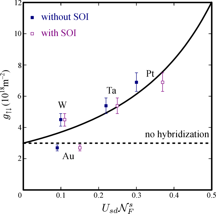
Figure 2 shows the enhancement of spin-mixing conductance of an insulating ferromagnet Y3Fe5O12 and a heavy metal (HM) as a function of . For Y3Fe5O12 with the magnetic moment and unit cell lattice constant Å[26, 27], spin-mixing conductance per unit area can be estimated to be
| (41) |
The result is in agreement with the experimental work of Ref. 25. This indicates that the - orbital hybridization induces an effective electron-electron interaction on the conduction electron of the heavy transition metal and increases the spin-mixing conductance at its interface with a ferromagnetic insulator.
The discussion so far focuses on the case when the ferromagnetic layer is insulating. In an insulating magnetic interface, the orbital hybridization dominates the scattering for the interface of a ferromagnetic insulator and heavy metal, because only the heavy metal contributes to the conduction electrons. However, in the case of a metallic ferromagnet, the interactions of a conduction electron near the interface is more complicated. For a metallic ferromagnet (e.g., cobalt), to capture the complexity of the heavy-metal system [14], the enhancement factor should be replaced by a phenomenological parameter of the Stoner model[29, 4].
| (42) |
where
| (43) |
is the unenhanced spin-mixing conductance of the bilayer of HM and Co with width Å[28], magnetic moment , and cell volume Å3 [26, 30].
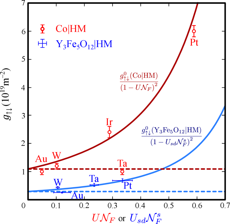
Figure 3 shows the agreement of Eq. 42 with the experiment of a metallic ferromagnet and Eq. (39) with the experiment of insulating ferromagnet. CoHM has a larger than Y3Fe5O12 because the conduction spin can penetrate into a metallic ferromagnet and interact with more magnetic moments. When the ferromagnet layer is an insulator, the conduction electron purely originates from the heavy transition metal. Therefore, - hybridization dominates the electron-electron interaction and our model is more appropriate.
IV Conclusions
To summarize, we discuss the effect of - orbital hybridization on the spin-mixing conductance of the interface of ferromagnet and heavy metal. Using a generalized Anderson model, we study the linear response theory of conduction spin near a magnetic interface. At the magnetic interface, the hybridization of the conduction electron and localized electron of a heavy transition metal increases of the spin susceptibility of a heavy transition metal and subsequently enhances the spin-mixing conductance of the interface of ferromagnetic and transition metal.
For a bilayer of a ferromagnetic metal and a heavy metal, the enhancement of spin-mixing conductance is characterized by electron-electron interaction parameter in Stoner model , as illustrated in Fig. 3. Meanwhile, for a bilayer of ferromagnet insulator and a heavy metal, the enhancement is characterized by the electron-electron interaction parameter due to orbital hybridization that depends on the hybridization energy and the dispersion of and electrons. These parameters can be obtained by analyzing the band structure obtained from DFT. Figure 2 shows the agreement of our theory and the experimental values of the bilayer of Y3Fe5O12 and transition metal.
Acknowledgements.
We thank Universitas Indonesia for funding this research through PUTI Grant No. NKB-469/UN2.RST/HKP.05.00/2022.Appendix: Energy dispersion and density of states of 5d transition metals
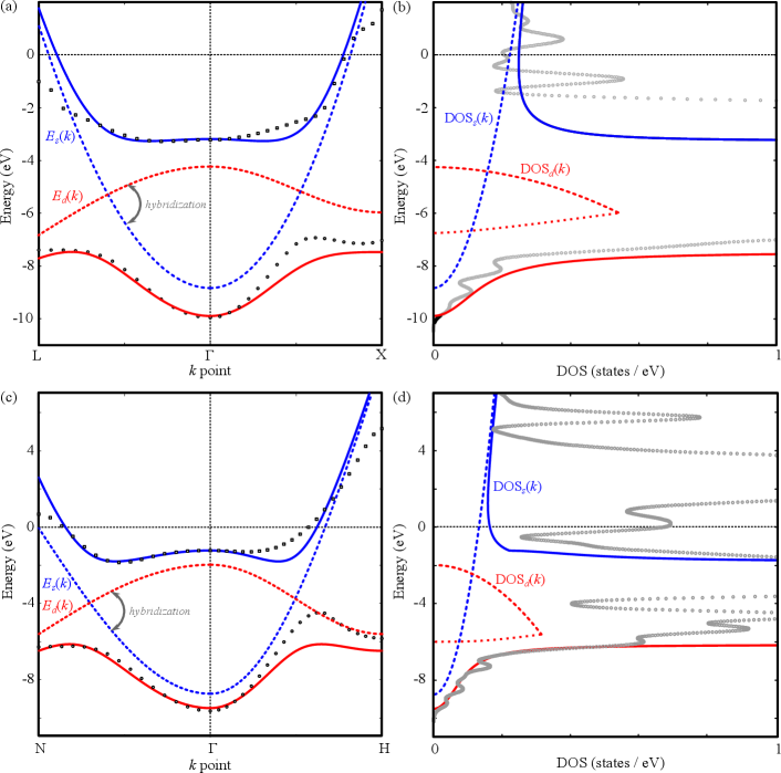
In this article we analyze the orbital mixing of Ta, W, Ir, Pt and Au. The orbital mixing occurs because of the hybridization between conduction ( band) and localized ( band, illustrated by DOSd) electrons [21]. The hybridized energy bands due to Hamiltonian in Eq. (13) are
| (44) |
As illustrated in Fig. 4, the partially filled band near the Fermi surface is chosen as , while the band at the bottom of the density of states is chosen as . Ir, Pt and Au have fcc structures. Figures 4(a) and 4(b) illustrate the band structure along LX symmetry points and density of states, respectively. On the other hand, Ta and W have bcc structure. Figures 4(c) and 4(d) illustrate the band structure along NH symmetry points and density of states, respectively.
By assuming and to be parabolic near point, the band structure parameters can be obtained by fitting the band structure obtained from DFT. The sum of and
| (45) |
can be used to obtain
On the other hand, their difference
| (46) |
can be used to obtain
and hybridization energy . The and effective masses can then be obtained from and , respectively.
References
- Barnaś et al. [2005] J. Barnaś, A. Fert, M. Gmitra, I. Weymann, and V. K. Dugaev, From giant magnetoresistance to current-induced switching by spin transfer, Phys. Rev. B 72, 024426 (2005).
- Brataas et al. [2017] A. Brataas, Y. Tserkovnyak, G. E. W. Bauer, and P. J. Kelly, Spin current (Oxford University Press, 2017) Chap. Spin Pumping and Spin Transfer.
- Xiao et al. [2008] J. Xiao, G. E. W. Bauer, and A. Brataas, Spin-transfer torque in magnetic tunnel junctions: Scattering theory, Phys. Rev. B 77, 224419 (2008).
- Cahaya and Majidi [2021] A. B. Cahaya and M. A. Majidi, Effects of screened coulomb interaction on spin transfer torque, Phys. Rev. B 103, 094420 (2021).
- Tserkovnyak et al. [2002a] Y. Tserkovnyak, A. Brataas, and G. E. W. Bauer, Spin pumping and magnetization dynamics in metallic multilayers, Phys. Rev. B 66, 224403 (2002a).
- Tserkovnyak et al. [2002b] Y. Tserkovnyak, A. Brataas, and G. E. W. Bauer, Enhanced gilbert damping in thin ferromagnetic films, Phys. Rev. Lett. 88, 117601 (2002b).
- Cahaya [2021] A. B. Cahaya, Antiferromagnetic spin pumping via hyperfine interaction, Hyperfine Interactions 242, 46 (2021).
- Cahaya [2022] A. B. Cahaya, Adiabatic limit of rkky range function in one dimension, J. Magn. Magn. Mater. 547, 168874 (2022).
- Carva and Turek [2007] K. Carva and I. Turek, Spin-mixing conductances of thin magnetic films from first principles, Phys. Rev. B 76, 104409 (2007).
- Šimánek [2003] E. Šimánek, Gilbert damping in ferromagnetic films due to adjacent normal-metal layers, Phys. Rev. B 68, 224403 (2003).
- Cahaya et al. [2017] A. B. Cahaya, A. O. Leon, and G. E. W. Bauer, Crystal field effects on spin pumping, Phys. Rev. B 96, 144434 (2017).
- Weiler et al. [2013] M. Weiler, M. Althammer, M. Schreier, J. Lotze, M. Pernpeintner, S. Meyer, H. Huebl, R. Gross, A. Kamra, J. Xiao, Y.-T. Chen, H. J. Jiao, G. E. W. Bauer, and S. T. B. Goennenwein, Experimental test of the spin mixing interface conductivity concept, Phys. Rev. Lett. 111, 176601 (2013).
- Santos et al. [2013] D. L. R. Santos, P. Venezuela, R. B. Muniz, and A. T. Costa, Spin pumping and interlayer exchange coupling through palladium, Phys. Rev. B 88, 054423 (2013).
- Zhu et al. [2019] L. Zhu, D. C. Ralph, and R. A. Buhrman, Effective spin-mixing conductance of heavy-metal–ferromagnet interfaces, Phys. Rev. Lett. 123, 057203 (2019).
- Sigalas and Papaconstantopoulos [1994] M. M. Sigalas and D. A. Papaconstantopoulos, Calculations of the total energy, electron-phonon interaction, and Stoner parameter for metals, Phys. Rev. B 50, 7255 (1994).
- Zellermann et al. [2004] B. Zellermann, A. Paintner, and J. Voitländer, The onsager reaction field concept applied to the temperature dependent magnetic susceptibility of the enhanced paramagnets Pd and Pt, J. Phys. Condens. Matter 16, 919 (2004).
- Povzner et al. [2010] A. A. Povzner, A. G. Volkov, and A. N. Filanovich, Electronic structure and magnetic susceptibility of nearly magnetic metals (palladium and platinum), Physics of the Solid State 52, 2012 (2010).
- Sitorus et al. [2021] R. M. Sitorus, A. Azhar, A. B. Cahaya, A. R. T. Nugraha, and M. A. Majidi, Theoretical study of complex susceptibility of pd and pt, Journal of Physics: Conference Series 1816, 012044 (2021).
- Anderson [1961] P. W. Anderson, Localized magnetic states in metals, Phys. Rev. 124, 41 (1961).
- Schrieffer and Wolff [1966] J. R. Schrieffer and P. A. Wolff, Relation between the Anderson and Kondo Hamiltonians, Phys. Rev. 149, 491 (1966).
- Goodenough [1960] J. B. Goodenough, Band structure of transition metals and their alloys, Phys. Rev. 120, 67 (1960).
- Clark et al. [2005] S. J. Clark, M. D. Segall, C. J. Pickard, P. J. Hasnip, M. I. J. Probert, K. Refson, and M. C. Payne, First principles methods using castep, Zeitschrift für Kristallographie - Crystalline Materials 220, 567 (2005).
- Giannozzi et al. [2009] P. Giannozzi, S. Baroni, N. Bonini, M. Calandra, R. Car, C. Cavazzoni, D. Ceresoli, G. L. Chiarotti, M. Cococcioni, I. Dabo, A. D. Corso, S. de Gironcoli, S. Fabris, G. Fratesi, R. Gebauer, U. Gerstmann, C. Gougoussis, A. Kokalj, M. Lazzeri, L. Martin-Samos, N. Marzari, F. Mauri, R. Mazzarello, S. Paolini, A. Pasquarello, L. Paulatto, C. Sbraccia, S. Scandolo, G. Sclauzero, A. P. Seitsonen, A. Smogunov, P. Umari, and R. M. Wentzcovitch, QUANTUM ESPRESSO: a modular and open-source software project for quantum simulations of materials, J. Phys. Condens. Matter 21, 395502 (2009).
- Pizzi et al. [2020] G. Pizzi, V. Vitale, R. Arita, S. Blügel, F. Freimuth, G. Géranton, M. Gibertini, D. Gresch, C. Johnson, T. Koretsune, J. Ibañez-Azpiroz, H. Lee, J.-M. Lihm, D. Marchand, A. Marrazzo, Y. Mokrousov, J. I. Mustafa, Y. Nohara, Y. Nomura, L. Paulatto, S. Poncé, T. Ponweiser, J. Qiao, F. Thöle, S. S. Tsirkin, M. Wierzbowska, N. Marzari, D. Vanderbilt, I. Souza, A. A. Mostofi, and J. R. Yates, Wannier90 as a community code: new features and applications, J. Phys. Condens. Matter 32, 165902 (2020).
- Wang et al. [2014] H. L. Wang, C. H. Du, Y. Pu, R. Adur, P. C. Hammel, and F. Y. Yang, Scaling of spin hall angle in 3d, 4d, and 5d metals from /metal spin pumping, Phys. Rev. Lett. 112, 197201 (2014).
- Jain et al. [2013] A. Jain, S. P. Ong, G. Hautier, W. Chen, W. D. Richards, S. Dacek, S. Cholia, D. Gunter, D. Skinner, G. Ceder, and K. a. Persson, Commentary: The Materials Project: A materials genome approach to accelerating materials innovation, APL Materials 1, 011002 (2013).
- Rodic et al. [1999] D. Rodic, M. Mitric, R. Tellgren, H. Rundloef, and A. Kremenovic, True magnetic structure of the ferrimagnetic garnet Y3Fe5O12 and magnetic moments of iron ions, J. Magn. Magn. Mater 191, 137 (1999).
- Ma et al. [2018] X. Ma, G. Yu, C. Tang, X. Li, C. He, J. Shi, K. L. Wang, and X. Li, Interfacial dzyaloshinskii-moriya interaction: Effect of band filling and correlation with spin mixing conductance, Phys. Rev. Lett. 120, 157204 (2018).
- Šimánek and Heinrich [2003] E. Šimánek and B. Heinrich, Gilbert damping in magnetic multilayers, Phys. Rev. B 67, 144418 (2003).
- Persson [2016] K. Persson, Materials data on Co (SG:194) by materials project (2016).