Enhanced Generator Coordinate Method: eGCM
Abstract
The generator coordinate method (GCM) was introduced in nuclear physics by Wheeler and his collaborators in 1950’s and it is still one of the mostly used approximations for treating nuclear large amplitude collective motion (LACM). GCM was inspired by similar methods introduced in molecular and condensed matter physics in the late 1920’s, after the Schrödinger equation became the tool of choice to describe quantum phenomena. The interest in the 1983 extension of GCM suggested by Reinhard, Cusson and Goeke, which includes internal excitations, was revived in recent years, but unfortunately this new time-dependent GCM (TDGCM) framework has a serious flaw, which prevents it from describing correctly many anticipated features in a properly formulated TDGCM framework, such as interference and entanglement. I present here an alternative formulation, the enhanced GCM (eGCM), which is free of difficulties encountered in previous TDGCM implementations and relevant for fission and many-nucleon transfer in heavy-ion reactions.
The early attempts to describe molecular spectra by W. Heitler, F. London, J. C. Slater, L. Pauling, and others used hybridized localized atomic orbitals, centered on atoms. Later F. Hund, R. S. Mulliken, and J. Lennard-Jones introduced delocalized molecular orbitals, which proved more flexible in practice. The atomic orbitals centered at atom positions describe electrons in various states, e.g. the and orbitals used to describe the valence electrons in a carbon atom. At each atomic site this set of orbitals is not complete and higher energy excitations of the system are thus not included. In the case of carbon atoms the excitation of the deep lying electrons with principal quantum numbers and or to levels with are not allowed. Whether this is a good approximation naturally depends on the specific problem considered, which typically encompasses relatively low energy local excitations of the quantum system under consideration. These ideas propagated further in condensed matter theory in order to describe the band structure of solids Aschroft and Mermin (1976) and lately in the high-temperature superconductivity in the Hubbard model Dong et al. (2022). Localized or delocalized orbitals describe electrons in various quantum states, including the spin degrees of freedom.
These ideas also inspired J. A. Wheeler and his students D. A. Hill and J. J. Griffin Hill and Wheeler (1953); Griffin and Wheeler (1957) to introduce a description of nuclear LACM, nuclear fission in particular, for which they coined the term GCM. These authors considered however a simplified version of the molecular and condensed matter frameworks, by using at “each site,” in that case for a particular nuclear shape typically characterized by a quadrupole and an octupole deformation , only the ground states of a nucleus with that shape, and the wave function of the nucleus was represented as a linear superposition of these fixed shape ground states. In nuclear literature the GCM was considered over the years in two flavors, with time-independent “generator wave function” function and with a time-dependent “generator wave function” respectively
| (1) | |||
| (2) |
but in both cases with static (generalized) Slater determinants Ring and Schuck (2004); Verriere and Regnier (2020); Schunck and Regnier (2022); Schunck (2022), as solutions of chosen by “educated guesses” of a restricted set of nuclear shape constraint Hartree-Fock (HF) or Hartree-Fock-Bogoliubov (HFB) solutions. These two choices are neither well nor uniquely defined and consequently the “sum” over “nuclear shapes” parametrized by the multidimensional variable lead to a uncontrolled approximation of the many-fermion wave function or , see Ref. sup . A correct expansion in terms of either static or time-dependent (generalized) Slater determinants should include all possible many-fermion excitations at a “given shape,” not only the “ground state” at a given “shape.” At the same time by including all excited states at all “nuclear shapes” will make the entire set overcomplete. In the literature, as far as I know, there is no study of the accuracy of the GCM or of the accuracy of the similar framework based on molecular orbitals. At best, studies demonstrate that there is “agreement” with a reduced set of observables, when a reasonable basis set of wave functions, chosen by educated guesses, is used.
Over the many decades of GCM use in nuclear physics, the belief, or rather the hope, has been that the total wave functions will follow an adiabatic evolution from one instantaneous “ground state shape” to the next neighboring instantaneous “ground state shape,” which led to the development of the adiabatic time-dependent Hartree-Fock theory Ring and Schuck (2004). In chemistry it has been known for decades that this naive Born-Oppenheimer approximation Born and Oppenheimer (1927) is violated Tully (1990). There are also other possible theoretical frameworks, see Refs. Requist and Gross (2016); Agostini and Gross (2020); Bulgac et al. (2019a); Bulgac (2022) and earlier references therein. In the case of nuclear LACM the nuclear shape has to evolve typically in low energy nuclear dynamics in such a manner that the local Fermi momentum distribution remains approximately spherical Bertsch (1980); Barranco et al. (1988, 1990); Bertsch and Flocard (1991); Bertsch and Bulgac (1997), as otherwise the volume contribution to the energy of the nucleus will change. Nuclear systems are saturating many fermion systems and in the low energy dynamics the contribution to the volume energy and the average density should remain essentially constant Meitner and Frisch (1939); Hill and Wheeler (1953); Bertsch (1980). Only the Coulomb and surface isoscalar and isovector contributions to the total nucleus energy can vary considerably, in agreement with the brilliant insight Meitner and Frisch (1939) had in the case of nuclear fission. The energy contribution due to the emergence of pairing correlations is always a small contribution, but however crucial. In the Bethe-Weiszäcker mass formula the odd-even correction term is about times smaller than the root mean square error of the binding energy of any nucleus with an atomic mass larger than . At a well defined “nuclear shape” a many nucleon system has a very rich spectrum of excited states, qualitatively similar to the various states of electron systems, or similar to the full spectrum of a nucleus described in a large shell model basis. While changing its shape a nucleus does not have to hop from one ground state of a given shape to another ground state of a different shape only. This “conspicuous” deficiency was attempted to be “fixed” in Ref. Müther et al. (1977); Bernard et al. (2011); Chen and Egido (2017), in an approach where only a patently insufficient number of excited states was taken into account. As far as I am aware this (uncontrollable) extension of GCM Bernard et al. (2011) was never shown to lead to a satisfactory description of LACM, and moreover, it is not clear whether such an extension is numerically feasible or practically meaningful if all relevant quasiparticle excitations are taken into account.
It is well established theoretically that LACM of a fissioning nucleus beyond the outer fission barrier is a strongly dissipative non-equilibrium process Bulgac et al. (2016, 2019b, 2020); Bender and et al. (2020) and the adiabaticity invoked by Wheeler and collaborators Hill and Wheeler (1953); Griffin and Wheeler (1957) is an unphysical assumption, which however is still widely used in GCM “microscopic” approaches to nuclear fission up to the scission configuration Verriere and Regnier (2020); Schunck and Regnier (2022); Schunck (2022). In theoretical studies of LACM in the first and second potential well, and in particular in the case of spontaneous fission Balantekin and Takigawa (1998); Sadhukahn (2020) the attitude is that the collective motion is adiabatic. The argument brought forward in the case of spontaneous fission, which is to a large extent an under the barrier penetration process, is that due to pairing effects the adiabatic approximation is valid. This goes against the solid theoretical arguments presented by Caldeira and Leggett (1983) and widely accepted in condensed matter physics, that the coupling to internal excitations (in nuclear language parlance, coupling to excitations above “the instantaneous ground shape” and when "polarization effects" are neglected) leads to longer tunneling times. This is in qualitative agreement with experimental observations of the spontaneous life-times of odd-mass and odd-odd nuclei Vandenbosch and Huizenga (1973), and also with our recent findings Bulgac (2024), where in particular we demonstrate that the Pauli blocking approximation is not valid in non-equilibrium processes and therefore Cooper pairs are broken during LACM.
In 1983 Reinhard et al. (1983) suggested to replace the static fixed set of ground states a nucleus evolves through during a LACM with the solutions of a time-dependent HF problem. In this framework the total time dependent nuclear wave function of the nucleus acquires a more complex structure, it is in general an infinite sum/integral over many (generalized) time-dependent Slater determinants . Allegedly, this prescription may describe a dissipative non-equilibrium process such as nuclear fission or heavy-ion reaction. In Ref. Reinhard et al. (1983) it was implicitly assumed that various TDHF trajectories are started simultaneously and span a sufficiently large set of initial nuclear shapes, described by the shape (multidimensional) parameter . The “generator wave function” is a solution of the time-dependent Hill-Wheeler equation
| (3) |
where the nucleon coordinates have been suppressed and the matrix elements and are evaluated by integrating over the coordinates . Here and stand for the many-body and mean field Hamiltonians, and .
In order to understand the incompleteness of the arguments presented by Reinhard et al. (1983) I have to make a detour to introducing in quantum many-body theory the collective and intrinsic degrees of freedom, a process described a long time ago by Feynman and Vernon (1963), from which either a classical Grangé et al. (1983); Weidenmüller and Zhang (1984) or quantum Fokker-Planck equation Bulgac et al. (1996, 1998); Kusnezov et al. (1999) for the “collective degrees of freedom” can be derived. In the GCM framework one typically interprets the (generalized) Slater determinants labels as a set of collective variables, thus practically introducing a poor man’s Feynman-Vernon separation between the “collective degrees of freedom ”, which need to be requantized, and the "intrinsic degrees of freedom ." In GCM this is achieved by adopting the Gaussian overlap approximation (GOA) Ring and Schuck (2004); Verriere and Regnier (2020); Schunck and Regnier (2022); Schunck (2022) of the norm and Hamiltonian overlaps and “deriving” a Schrödinger-like equation for the “collective degrees of freedom .” In the most theoretically advanced implementation of the TDDFT extended to superfluid systems Bulgac et al. (2016, 2019b, 2020), as in any previous time-dependent mean field approach the “collective degrees of freedom ” are simply labels for the initial conditions in case of time-dependent problems. Mixing different (TD)DFT trajectories requires knowledge of the function either or , which can be obtained only by solving the corresponding static or time-dependent GCM equations or using other phenomenological or microscopic approaches Wilkins et al. (1976); Brosa et al. (1990); Lemaître et al. (2015); Ishizuka et al. (2017); Sierk (2017); Albertsson et al. (2020); Ivanyuk et al. (2024); Sadhukhan et al. (2016, 2017); Sadhukhan (2020).
A very instructive example of a GCM-like application, though it was never considered as one, is the treatment of pairing correlations, and specifically the treatment of a bound electron pair by Cooper (1956). The pairing Hamiltonian in second quantization is
| (4) |
and the electron pair wave function is , with a sum over two-fermion Hartree-Fock states in time reversed states and , and here the coefficients are obtained as solution of a GCM-like equation, in which the norm overlap is diagonal, while the Hamiltonian overlap is not and leads to hops between different “generator coordinate” states , where is the vacuum state. In GCM calculations the basis states are not typically orthogonal to each other and the norm overlap as a result is non-diagonal, which leads to the usual technical problems. One can extend trivially Cooper (1956)’s treatment of a single pair to several pairs, but when the number of pairs one should switch to the Hartree-Fock-Bogoliubov (HFB) approximation.
There were a few attempts in recent literature Regnier and Lacroix (2019); Hasegawa et al. (2020); Marević et al. (2023, 2024); Li et al. (2023, 2024) to implement the framework suggested by Reinhard et al. (1983), but the results obtained so far have not shown how to obtain the expected mass and charge distributions of fission fragments (FFs) or how to describe an expected effective mixing between different trajectories Li et al. (2024), or with a better accuracy than in a quite wide variety of other approaches Wilkins et al. (1976); Brosa et al. (1990); Lemaître et al. (2015); Ishizuka et al. (2017); Sierk (2017); Albertsson et al. (2020); Ivanyuk et al. (2024); Sadhukhan et al. (2016, 2017); Sadhukhan (2020).
There are several reasons why the framework outlined by Reinhard et al. (1983) is not going to succeed in describing the non-equilibrium dynamics of a many-fermion systems, since the initial conditions are not well defined. As shown in Refs. Bulgac et al. (2019b, 2020), fission trajectories started along the rim of the outer fission barrier, after a very short time appear to focus into a rather narrow bundle. Unfortunately these trajectories reach a particular set of FF separations at different times, as the saddle-to-scission times vary quite a bit, depending on the initial values of , and as a result the norm and Hamiltonian overlaps evaluated of a given time , counted from the time each specific trajectory was started, leads to practically vanishing values of the Hamiltonian overlaps and therefore to no “expected quantum mixing”’ between different trajectories parametrized by the “classical variables ” Li et al. (2024). This is very similar to the Thomas Young two-slit or the Mach-Zehnder experiments, with either light waves or quantum objects, when particles hit the screen and interfere after traveling for different times along different trajectories and hit a spot on the screen after different times spent from the emission. This is the main element overlooked by Reinhard et al. (1983). In induced fission an incident low energy neutron beam excites the system in its ground state potential well and different “classical trajectories,” described by the “collective variables ,” reach the rim of the outer fission barrier at different times and eventually the FF detector, the “screen,” where the interference occurs.
The solution to this apparently complicated problem is rather simple, see also the supplement sup . There a number of relevant references are listed Peierls and Yoccoz (1957); Peierls and Thouless (1962); Ryssens et al. (2015); Bulgac (2013); Bulgac et al. (2018, 2021, 2022); Scamps et al. (2023); Zagrebaev et al. (2013); Sekizawa and Yabana (2013); Berry (1984); Bulgac (1988, 2024); Barrett et al. (2013); Scharnweber et al. (1971); Bulgac (1989); Taylor (1909); Merli et al. (1976); Arndt et al. (1999); Hanbury Brown and Twiss (1956); Boal et al. (1990); Bell (1987), a relation to the old works of Peierls and Yoccoz (1957) and Peierls and Thouless (1962) is presented and discussed how very strong correlations, absent in mean field, are generated. Instead of the norm and Hamiltonian overlap matrix elements in Eq. (3) one should evaluate the new generalized norm and the Hamiltonian overlap matrix elements and solve the extended GCM (eGCM) equations
| (5) |
using the variational approach with the eGCM many-body wave function , which is akin to Feynman path integral representation sup . One can introduce the separation between FFs along each TDDFT trajectory Bulgac (2019); Bulgac et al. (2019b); Bulgac (2013) as a function of time . The new norm and the Hamiltonian overlaps are non-vanishing if is similar in magnitude to , in the case of fission of an axially symmetric nucleus, when the FFs are in close proximity of each other sup . Note that TDDFT is used to generate a physically sound choice set of many-body wave functions (analogous to the set of harmonic single-particle wave functions used in shell model calculations, and which is desirably complete sup for a controlled approximation) and they do not have to be related with the Hamiltonian used in Eq. (Enhanced Generator Coordinate Method: eGCM), unlike in (TD)GCM applications Verriere and Regnier (2020); Schunck and Regnier (2022); Schunck (2022). eGCM is capable of describing interference patterns in the detector, even though particles arriving by different paths and at different times , a fact known otherwise for a very long time sup ; Taylor (1909); Merli et al. (1976); Arndt et al. (1999).
It is instructive to develop an intuition concerning the meaning and importance of the parameters and important to discuss the feasibility of implementing eGCM. In an analogy with with a non-uniform diffraction grating with a finite number of slits, one can associate with the label of a specific slit, in this case including not only the position of the initial point on the rim of the outer barrier, but if desired also the Euler angles specifying of the fissioning nucleus needed to perform an angular momentum projection.
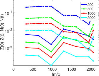
In the case of generalized Slater determinants used in the case of induced fission one has to include all allowed quasiparticle states in constructing a time-dependent “trajectory,” see Ref. Bulgac et al. (2024a), which for a typical situation in a box fm3 and a lattice constant , which is a very large number = 216,000, unlike in all known to us real-time numerical simulations of fission used by other authors in literature so far. Fortunately, there is a solution to this problem, at each specific set of values one should introduce the canonical wave functions and in that case the size of the needed number of quasiparticle wave functions dramatically drops to a several hundreds, see Fig. 1 and Refs. Scamps et al. (2023); Bulgac et al. (2024a), and the needed norm and Hamiltonian overlaps can be evaluated rather rapidly.
I will assume that one performs induced fission simulations in a typical ( fm)3 box, if angular momentum projection is considered. Otherwise a fm3 simulation box is appropriate. For evaluating the first and second spatial derivatives the use of FFT, which leads to machine precision and using powers of 2 is the best choice for spatial dimensions Jin et al. (202); Bulgac et al. (2011). The lattice constant fm corresponds to a maximum momentum cutoff in one cartesian direction 600 MeV/c, which is of the order of the maximum momentum cutoff considered in chiral effective field theory of nucleon interactions. It would be sufficient to use a number for the set of quadrupole and octupole deformations for an axially symmetric even-even compound nucleus along the rim of the outer fission barrier, as was done in Refs. Bulgac et al. (2016, 2019b, 2020). Sometimes it maybe convenient to parameterize a given trajectory in terms of the separation between FFs, starting with a separation fm, when the neck is emerging, until fm, when the FF shapes are relaxed and spatially rather well separated, and use the relation between the time along the trajectory and the FFs separation , where is the running time along a given trajectory. Retaining for the eGCM a fm one would need different FFs separations along a given trajectory. As it was amply demonstrated recently, see again Fig. 1 and Refs. Scamps et al. (2023); Bulgac et al. (2024b, c), it is sufficient to use not more than hopefully canonical wave functions with the highest occupation probabilities, for the proton and neutron subsystems respectively.
If one might try instead to eschew the determination of the canonical wave functions and use instead quasiparticle wave functions with the highest occupation probabilities at each FF separation , or use a static or time-dependent Bardeen-Cooper-Schrieffer approximation, the errors are large, essentially irrespective of how many states are included. A further simplification of the eGCM framework can be achieved by adopting an appropriate generalized Gaussian overlap approximation (GOA) for the norm kernel and derive a Schrödinger-like equation for . The GOA is however a further approximation, prone to large errors Verrière et al. (2017), and it was prompted only to find a simple simulacrum to a “collective Hamiltonian quadratic in collective coordinates” to the Feynman-Vernon influence functional, which emerges from a path integral formulation of the many-body problem. As it was shown in Ref. Bulgac (1988), in the case of nonlocal equations a reduction to a second order partial differential equation is not always possible, as the system has a behavior similar to a birefringent medium.
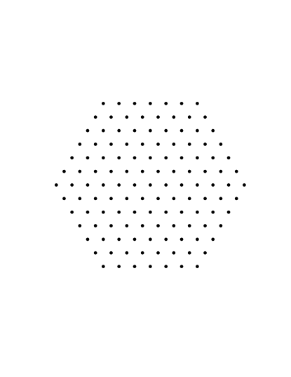
In the case of fissioning even-even nuclei with axial symmetry one can build a rather simple angular momentum projection procedure of the nucleus as only the Euler angles and are needed and one can use the icosahedral group with only 60 different angles to project on the total spin and 2, using the positions of the 60 carbon atoms in a buckyball for different orientations of the “collective” variables . This approach is orders of magnitude more economic that the usual angular momentum projecting techniques Ring and Schuck (2004); Lu et al. (2022); Scamps et al. (2023). This leads to a conservative estimate of the dimension of the norm overlap matrices (separately for protons and neutrons) , which is a number significantly smaller than the largest dimensions of the shell-model calculations Johnson (2018); Zbikowski and Johnson (2023). If an angular momentum projection is not performed the dimension of norm overlap matrices is significantly smaller . Since only the largest eigenvalues of the norm overlap matrices are needed, full diagonalization is not necessary. As it was recently shown in Ref. Bulgac et al. (2024b), the differences between the number-projected and number-unprojected number densities as a function of time at any point in space are at most at the level 1 in the case of induced fission treated in TDDFT with pairing correlations included, during the entire time-evolution from the top of the outer fission barrier to complete fission fragments (FFs) separation. Naturally, this new eGCM framework is equally applicable to other cases of nuclear LACM, in particular to collisions of heavy ions. Since the emergence of powerful supercomputers during the last two decades or so, the numerical implementation of eGCM appears to be doable with many existing and rather modest computer platforms.
The most contentious and difficult issue in using GCM in nuclear LACM is the fact that, in DFT and in TDDFT in particular, a true Hamiltonian does not exist and the evaluation of the Hamiltonian overlap within GCM is not well defined. The Hamiltonian overlaps in Eq. (Enhanced Generator Coordinate Method: eGCM) should and can be be evaluated using a true many-body Hamiltonian with two- and three-body interactions, when the evaluation of the norm and Hamiltonian overlaps with generalized mean field many-body wave functions is a well defined procedure Ring and Schuck (2004); Bertsch and Robledo (2012); Carlsson and Rotureau (2021), which has no ambiguity and eGCM can be used with generator wave functions from TDDFT as outlined above and in the supplement sup .
In conclusion, I have outlined an extended GCM framework, dubbed eGCM, which is free of a number of undefined steps in previous formulations, which is expected to correctly describe interference and entanglement between different “classical” fission trajectories, parametrized by the initial shapes on the rim of the outer fission barrier and different Euler angles and . Since rather soon after scission many TDDFT fission trajectories follow a very similar path Bulgac et al. (2019b, 2020), different trajectories originating at different initial points will find themselves in relatively close proximity of each other, albeit each parametrized with a different “time” , which translates into to an actual FFs separation . Having many different trajectories in close proximity of each other will result into a strong mixing, a fact which seemed almost impossible to realize until now Li et al. (2024). Since LACM dissipation is now organically incorporated in TDDFT extended to pairing correlations, there seem to be no other limitation to a full microscopic approach to fission. The only nagging element is that by construction GCM and equally the method of delocalized orbitals in chemistry and condensed matter physics are still uncontrollable approximations, even though the framework is based on sound physical assumptions.
Acknowledgements
I thank I. Stetcu, I. Abdurrahman, and M. Kafker for discussions, L. Troy, I. Abdurrahman, and M. Kafker for reading and suggesting a number of improvements, I. Abdurrahman for preparing the data for Fig. 1, and also D. Vretenar for raising number of questions on an earlier version of the manuscript. The funding from the Office of Science, Grant No. DE-FG02-97ER41014 and also the partial support provided by NNSA cooperative Agreement DE-NA0003841 is greatly appreciated. This research used resources of the Oak Ridge Leadership Computing Facility, which is a U.S. DOE Office of Science User Facility supported under Contract No. DE-AC05-00OR22725.
I Supplement to: Enhanced Generator Coordinate Method: eGCM
In the main text I have stated that various GCM frameworks introduced in nuclear physics, along with the more elaborate methods developed in the late 1920s for molecular and condensed matter systems, are uncontrolled approximations, since for a controlled approximation one would expect that the following relation is satisfied
| (6) | |||
| (7) |
which does not happen in any implementation of GCM. It is well known Ring and Schuck (2004) that the norm overlap does not have a proper inverse and has to be evaluated by excluding its zero-eigenvalues. As Eq. (6) is not an equality in any GCM framework considered so far, it implies that a many-body wave function cannot be exactly represented in this manner, unless all possible “nuclear shapes” are included, apart from the ground state at shape or even along with only a reduced number of “locally” excited states. No recipe for an appropriate “upper cut-off” on such “nuclear shapes” has ever been proven or justified in practice, except by “achieving” agreement with observations for some observables in model calculations. Reproducing with some accuracy energies of many-body states does not guarantee that all matrix elements of interest are accurate as well, as is the case in any variational approach.
While in either static GCM or TDGCM one introduces many-body wave functions
| (8) | |||
| (9) |
Reinhard et al. (1983) advocated the introduction a different type of many body wave functions
| (10) |
where are in general solutions of TDHF or TDDFT equations respectively. typically stands for average of the corresponding multipole quantum operators evaluated with the adopted GCM generator coordinate wave functions . In the case of either Eq. (8) or (9) is always time independent. The time independence of is implied in Eq. (10) and in Refs. Reinhard et al. (1983); Regnier and Lacroix (2019); Hasegawa et al. (2020); Marević et al. (2023, 2024); Li et al. (2023, 2024) and then can be interpreted as the expectation value of at evaluated with the chosen TDHF/TDDFT many-body wave functions , which thus are merely the “labels” analogous to various “slits in a many-slit interference experiment.”
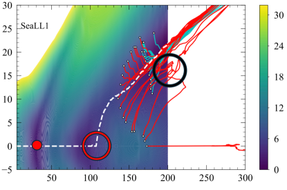
Fig. 2 is a slightly modified version of a figure published in Ref. Bulgac et al. (2019b). This figure illustrates several trajectories obtained using TDDFT extended to superfluid fermionic systems and used to describe the induced fission of 240Pu, using the energy density functional SeaLL1 Bulgac et al. (2018). All such TDDFT trajectories are mean field in character and, as well known in literature, at the same time classical trajectories. As demonstrated in Refs. Bulgac et al. (2016, 2019b), before scission the “collective motion” in the space is very slow and thus leads to very different travel times at which the fissioning nucleus arrives and also leaves the region bordered by the black circle following different trajectories and eventually FFs are captured in detectors.
In the arguments presented by Reinhard et al. (1983), and followed by subsequent authors Regnier and Lacroix (2019); Hasegawa et al. (2020); Marević et al. (2023, 2024); Li et al. (2023, 2024), in each set the trajectories are assumed to start at the same time and are solutions obtained in some mean field, which in particular could be a TDDFT framework as in Refs. Bulgac et al. (2016); Bulgac (2013, 2019); Bulgac et al. (2019b), but that does not have to be a requirement as one can easily argue, see below. Both the norm overlap kernel and most importantly the Hamiltonian kernel overlap in Reinhard et al. (1983) TDGCM equation
| (11) |
will be very small and thus negligible, as for the corresponding sets of “collective variables” and correspond the dramatically different nucleon spatial distributions typically. No significant mixing between various mean field TDDFT trajectories will thus occur in the scheme of Reinhard et al. (1983) if , while they are naturally included in an eGCM framework
| (12) |
as illustrated also with the example of the framework of Peierls and Yoccoz (1957), designed however only to restore symmetries in static calculations and discussed below.
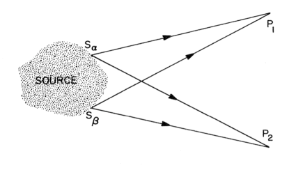
In an FF detector, FFs arriving along different trajectories and at different times are expected to interfere, in analogy with the many-slit interferometer discussed in the main text. In the two-slit or many-slits experiments a point on the screen it reached by two or several rays emitted as a rule at different times and which travel along different paths as well. This is a typical situation known for a very long time for photons, electrons, C60 molecules Taylor (1909); Merli et al. (1976); Arndt et al. (1999) and at astrophysical scales Hanbury Brown and Twiss (1956). The interference pattern can be observed when the intensity of the bean is extremely low and particles arrive at the screen/detector at different times, and thus obviously , an aspect fully neglected in the framework devised by Reinhard et al. (1983) or any other current theoretical treatment of fission or heavy-ion collisions.
FFs emerge in a quantum description from combining different TDDFT trajectories, which typically reach a detector at different times , exactly as in the two-slit experiment with very low intensity beams. In the case of nuclear fission one has however “two screens,” one, the detector for the light FF and the other, the detector for the heavy FF, each detector performing a projection/collapse/measurement from the many-body wave function
| (13) | |||
| (14) |
where is a projection operator on the spatial region of the corresponding either HFF (heavy) or LFF (light) FF detector. This set-up is thus similar to the Alice and Bob arrangement in measuring entanglement between two particles. This type of measurement can be defined to detect not only the FF position or arrival time in the detector, but also its spin, proton and/or neutron numbers, kinetic energy, excitation energy, etc. and eventually extract various entanglement aspects of the fission process. Along each TDDFT trajectory the FF configurations are uniquely identified by the initial values of the “collective coordinates” and the time when they reach the detector and the eGCM many-body wave function, see Eq. (13), describes the quantum superposition of these different contribution. In this respect Eq. (13) is a faithful Feynman path integral representation of the many-body wave function, where each component represents the final state followed by the quantum system along a specific “mean field classical path” and the corresponding weight of each component is determined by Eq. (12). Since as is well known from other interference experiments the interference pattern is independent of the intensity of the “FF beams,” and it exists even if FFs arrival times in the detectors Taylor (1909); Merli et al. (1976); Arndt et al. (1999); Hanbury Brown and Twiss (1956) and such techniques have been used in nuclear physics as well Boal et al. (1990). An obvious challenge for experiments is to properly set up the detectors so as to reveal the existence of various interference patterns and particularly to measure the FF entanglement Bell (1987).
In the case of neutron induced fission reaction likely the best choice would be to start all trajectories at the moment the incident neutron has been captured, the big red dot in Fig. 2, or even earlier, and follow all possible TDDFT “classical trajectories,” some of them in imaginary time, to the corresponding initial positions illustrated by white dots in Fig. 2. Such an approach has been used in Refs. Sadhukhan et al. (2016, 2017) to describe the spontaneous fission of 240Pu, by combining a semiclassical approach for the tunneling under the barrier, starting only in the second fission well however, with a classical Langevin approach from the outer turning point. In Refs. Sadhukhan et al. (2016, 2017) only the probabilities to arrive at the outer turning points have been used and not their quantum amplitudes, as it would have been the proper procedure in a quantum description. This treatment is equivalent to fully neglecting the quantum interference of such trajectories, as that would be needed in the case of diffraction from several “slits,” and this omission leads thus to a lack of accounting for all the possible particle transfers between two trajectories and also their quantum entanglement, when their corresponding ”collective coordinates” and are relatively close. This aspect is also clear from the analysis of the Peierls and Yoccoz (1957) symmetry restoration procedure, which leads to very strong quantum correlations, see the discussion of Eqs. (21, 22) below, correlations which are otherwise ignored.
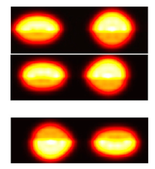
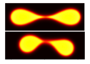
In Figs. 3 and 4 I illustrate a couple of different shape mixings, which are included in the eGCM framework. In the upper two panels are the nucleon distributions obtained as illustrated in Fig. 2, where the heavy FF is on the right and the light FF is on the left. While a mixing between shapes illustrated in the upper two panels of Figs. 3 could be included (but were not included so far beyond the scission configuration) in static GCM or its time-dependent extensions Reinhard et al. (1983); Verriere and Regnier (2020), a mixing between one configuration in either one of the upper two panels and another opposite configuration the third panel were not ever considered. The importance of such mixing is discussed below in relation with the work of Peierls and Yoccoz (1957). The nuclear shapes in the third panel of Fig. 3 were obtained by a simple reflection along the fission axis. Most likely such overlaps will be important before scission, particularly inside the region bordered by the red circle in Fig. 2, where the nucleus starts developing left-right asymmetry Ryssens et al. (2015), when , and the nucleus is still “confused” about which path to follow, to either or to . The quantum interference between different trajectories in the region where the fissioning nucleus becomes unstable with respect to left-right reflection can affect the probability that the heavy FF will end up either on the right or on left of the scission configuration. In this case, the FF on the left is a superposition of both the heavy and the light FFs, as in the case of the Schrödinger’s cat, which is both alive and dead at the same time. Another very important type of mixing between axially symmetric and axially non-symmetric configurations Bulgac et al. (2019a) illustrated in Fig. 4 was also never considered before in any GCM calculations and it should be included in future studies. The importance of including twisting and particularly bending FF modes in fission, which also can lead to such axially asymmetric configurations, was demonstrated by their presence in fission in recent microscopic studies of the FF intrinsic spins and their correlations Bulgac et al. (2021, 2022); Scamps et al. (2023).
The spirit of GCM is to consider overlaps between states with more or less similar values of , for example as those in the region inside the black circle in Fig. 2. In traditional GCM simulations Verriere and Regnier (2020); Schunck and Regnier (2022); Schunck (2022) only mixing of ground states at different values before the scission were considered. Mixing between configurations illustrated in Figs. 3 and 4 will account for particle transfer in various stages of heavy ion collision, after the reaction partners have experienced various stages of non-equilibrium evolution. Another type of mixing is in the case of heavy-ion collisions discussed below and the consideration of all possible impact parameters illustrated in Fig. 6. This type of mixing will be very important in the study of heavy-ion collisions Zagrebaev et al. (2013); Sekizawa and Yabana (2013) and it is similar in spirit to the mixing suggested a long time ago by Peierls and Yoccoz (1957) in order to restore translational invariance, see discussion below. These configurations are similar to the Cooper pair case discussed in the text, when the electron pairs jump from one site to another, however in this case from one reaction partner to the other during their non-equilibrium evolution. As in the case of Cooper pairs, the jumps between many “site” are crucial, as the effect of such jumps increases with the length of the chain one can jump on, and weakly depends on the width of the norm overlap kernel , which in the case of usual treatment of Cooper pairs is vanishing. The two FF configurations illustrated in Fig. 4 are positioned spatially in very close proximity and at different times.
These cases appear as quite surprising, as they are pure quantum effects. In a classical picture after the separation each FF has a well defined particle number. However, in a quantum world each FF is in a superposition of the FF being in the above and lower panel in Fig. 3, and these configurations can belong to the same TDDFT trajectory or to two different TDDFT trajectories, and the FFs might have different proton and neutron numbers as well. This is similar to pairs in the Cooper pair problem, when a pair is at one or another site according to what the exact wave function of the Copper pair tells us. However, with the important difference that now the “Cooper pair” can be in the ground state or in an excited state at either of these positions. In a similar manner, in a quantum world one has a superposition of one of the configurations in one of the upper panels in Fig. 3 with the the configuration in the third panel, particularly before scission, which is indeed a totally unexpected result of the quantum description. This type of mixing is more efficient near a configuration of the fissioning nucleus where an instability occurs, as in the case when the fission path becomes unstable against left-right reflection symmetry in the second fission well Ryssens et al. (2015). A similar situation was observed in Ref. Bulgac (2019) when considering symmetric splitting, and near such a point on the fission path the fission nucleus “gets confused on which direction to choose and spends a lot of time making up its mind.” Another similar situation was observed in the fission of odd nuclei when the odd particle was initially in a state with low quasiparticle energy, and when the fission time increases significantly Bulgac (2024).
Let me consider now a heavy ion imping on another heavy nucleus. The TDDFT wave function of the projectile before contact occurred, using the simplified notation used in Ref. Peierls and Yoccoz (1957), focusing on spatial coordinates only, is
| (15) | |||
| (16) |
where is the momentum of one nucleon, , stand for all nucleon spatial coordinates, is the impact parameter, , and is a (generalized) Slater determinant of a nucleus in its rest frame. The irrelevant factor was called by Berry (1984) the dynamical phase factor, see also Ref. Bulgac (1989),
| (17) |
can be absorbed into the function in eGCM. The wave function is accurate as long as the nucleus is moving in a straight line, thus very far from the target. In the case of the collision of two nuclei one should consider two such initial wave functions for each of the reaction participants and the total wave function of the system is a product of these separate wave functions.
Peierls and Yoccoz (1957) and Peierls and Thouless (1962) presented arguments which have some similarity to the arguments I outlined in the main text, while they were concerned only with restoring symmetries of the mean field many-body wave functions of stationary states. I will limit here the discussion to incident trajectories of a heavy-ion impinging on a target with different impact parameters, see Fig. 6. Peierls and Yoccoz (1957) argued that the translational symmetry of a stationary state mean field/TDDFT wave function of a nucleus at rest can be restored by considering the many-body wave function
| (18) |
where is the translational invariant wave function of a nucleus at rest, , and . It is important to appreciate that the wave function in Eq. (18) allows for mixing between mean field/TDDFT trajectories, in which a nucleon can jump from a site at an impact parameter and location along the -axis to another site on a different trajectory in a similar manner as a Cooper pair discussed in the main text, see Eq. (4) there, can jump from a site to another site , either in momentum or position space, depending on momentum or coordinate representation of the Cooper pair wave function.
As far as I am aware such jumps have never been considered in any theoretical treatments of heavy-ion collisions, and obviously such components of the incident and outgoing heavy-ion wave function are important, see Eqs. (21, 22) and the corresponding discussion. Later, Peierls and Thouless (1962) presented arguments in favor of introducing a further set of generator coordinates, describing the fluctuations of the nucleus center-of-mass trajectory, which in this case is a strict straight line. To this end Peierls and Thouless (1962) introduced velocity fluctuations of the nucleus center-of-mass with the more general approach
| (19) |
where the distribution of the nucleus center-of-mass velocities is determined from a variational principle, which I will consider below only for the Peierls and Yoccoz (1957) form, without center-of-mass velocity fluctuations .
It is instructive to see how the Peierls and Yoccoz (1957) ansatz, see Eq. (18) introduces correlations between particles for a simple mean field many-body wave function . Consider particles in harmonic oscillator single-particle states (), when the corresponding mean field, the symmetry restored two-particle density matrix and many-body wave functions are
| (20) | |||
| (21) | |||
| (22) |
where is the 2-body reduced density matrix for any function of type Eq. (22) with . Formally, this mechanism of generating correlations is similar to the Cooper pair mechanism discussed in the main text. The enforcement of Galilean invariance leads to a translationally invariant many-body wave function, similar to the no core shell model framework many-body wave function Barrett et al. (2013). It might be useful to compare this approach suggested by Peierls and Yoccoz (1957) to construct translational invariant “Slater determinants” to the method used in no core shell model calculations Barrett et al. (2013). eGCM thus becomes also formally equivalent to a no core shell model approach to fission and heavy-ion collisions, advocated a long time ago Scharnweber et al. (1971). The mixing of TDDFT trajectories is thus expected to lead to strong particle correlations beyond mean field.
Consider also the simpler case discussed by Peierls and Yoccoz (1957); Peierls and Thouless (1962) for which the corresponding equation for a stationary state of a nucleus is obtained from the GCM equations obtained by minimizing the total energy of the nucleus Peierls and Yoccoz (1957) (again, using their simplified notation)
| (23) |
This result from Ref. Peierls and Yoccoz (1957) is obtained by varying only in the many-body wave function
| (24) |
with the obvious solution satisfying Galilean invariance
| (25) |
Without including the fluctuations of the center-of-mass of the nucleus Peierls and Thouless (1962) the Hamiltonian overlap does not play a role in the evaluation of the total many-body wave function of the nucleus with total momentum and the energy in Eq. (23) is an improved beyond mean field variational estimate.
For a moving heavy-ion in eGCM one needs to rewrite Eq. (18) in a frame where the symmetry breaking of a many-body wave function is now in a moving reference frame. For a heavy-ion moving in the -direction with velocity , and the initial mean field many-body wave function is
| (26) | |||
| (27) |
and in Eq. (27) is the symmetry restored many-body wave function of an isolated moving heavy-ion. In the eGCM framework, the solution of the TDDFT equations for an isolated and moving heavy-ion , see Eq. (15), is related to , which can be brought easily into the form advocated in the main text. In Eq. (27) the integral over the third dimension in becomes an integral over time after the trivial change of variable . The equivalent of is now the 2D impact parameter , see Fig. 6 and thus . In a numerical simulation the integration in time and over the impact parameters can not extend beyond the limits when the reaction partners approach the walls of the simulation box. As in any numerical simulation, such as in lattice QCD for example, the size of the simulation box has to be chosen with appropriate care. Consequently, the eGCM form of the many-body function of the isolated heavy-ion has exactly the form advocated in the main text, namely
| (28) |
This particular type of TDDFT trajectories mixing and their effect on the many body wave function, which induces very strong correlations between particles, as is illustrated by the simple case discussed above, was clearly missed by the authors of Ref. Reinhard et al. (1983). It is worth noting that Reinhard et al. (1983) recognized the presence of pairs of trajectories which are “time-shifted,” but their proposed solution is clearly not adequate. The eGCM with generator coordinates incorporates naturally a large variety of mixing types between various TDDFT trajectories.
It is important to appreciate the fact, that in analogy with the Cooper pair discussed in the main text, a nucleon can in principle travel a long distance by jumping between different mean field/TDDFT trajectories. The number of different trajectories a nucleon can jump among depends on two factors: i) the first factor is the length of the path a nucleon is allowed to travel; ii) the other very important factor is the strength of the nucleon-nucleon interaction, which determines the time it takes to jump from one trajectory to another, which has to be compared with the extent of time of the entire reaction. In a macroscopic superconductor in a stationary state a Cooper pair has an infinite time to travel the entire length of the sample, but that is not the case in a nuclear reaction, where the time available for such jumps is limited.
References
- Aschroft and Mermin (1976) N. W. Aschroft and N. D. Mermin, Solid State Physics (Saunders College, 1976).
- Dong et al. (2022) X. Dong, L. Del Re, A. Toschi, and E. Gull, “Mechanism of superconductivity in the Hubbard model at intermediate interaction strength,” Proc. Nat. Acad. Sci 119 (33), e2205048119 (2022).
- Hill and Wheeler (1953) D. L. Hill and J. A. Wheeler, “Nuclear Constitution and the Interpretation of Fission Phenomena,” Phys. Rev. 89, 1102 (1953).
- Griffin and Wheeler (1957) J. J. Griffin and J. A. Wheeler, “Collective Motions in Nuclei by the Method of Generator Coordinates,” Phys. Rev. 108, 311 (1957).
- Ring and Schuck (2004) P. Ring and P. Schuck, The Nuclear Many-Body Problem, 1st ed. (Springer-Verlag, Berlin Heidelberg New York, 2004).
- Verriere and Regnier (2020) M. Verriere and D. Regnier, “The Time-Dependent Generator Coordinate Method in Nuclear Physics,” Front. Phys. 8, 233 (2020).
- Schunck and Regnier (2022) N. Schunck and D. Regnier, “Theory of nuclear fission,” Prog. Part. Nucl. Phys. 125, 103963 (2022).
- Schunck (2022) N. Schunck, “Microscopic Theory of Nuclear Fission,” (2022), arXiv:2201.02716 [nucl-th] .
- (9) “Supplemental material, link to be added by publisher.” .
- Born and Oppenheimer (1927) M. Born and R. Oppenheimer, “Zur Quantentheorie der Molekeln,” Annalen der Physik 389, 457 (1927).
- Tully (1990) J. C. Tully, “Molecular dynamics with electronic transitions,” J. Chem. Phys. 93, 1061 (1990).
- Requist and Gross (2016) R. Requist and E. K. U. Gross, “Exact Factorization-Based Density Functional Theory of Electrons and Nuclei,” Phys. Rev. Lett. 117, 193001 (2016).
- Agostini and Gross (2020) F. Agostini and E. K. U. Gross, “Exact Factorization of the Electron–Nuclear Wave Function: Theory and Applications,” in Quantum Chemistry and Dynamics of Excited States (John Wiley and Sons, Ltd, 2020) Chap. 17, p. 531.
- Bulgac et al. (2019a) A. Bulgac, S. Jin, and I. Stetcu, “Unitary evolution with fluctuations and dissipation,” Phys. Rev. C 100, 014615 (2019a).
- Bulgac (2022) A. Bulgac, “Pure quantum extension of the semiclassical Boltzmann-Uehling-Uhlenbeck equation,” Phys. Rev. C 105, L021601 (2022).
- Bertsch (1980) G. Bertsch, “The nuclear density of states in the space of nuclear shapes,” Phys. Lett. B 95, 157 (1980).
- Barranco et al. (1988) F. Barranco, R. A. Broglia, and G. F. Bertsch, “Exotic radioactivity as a superfluid tunneling phenomenon,” Phys. Rev. Lett. 60, 50 (1988).
- Barranco et al. (1990) F. Barranco, G.F. Bertsch, R.A. Broglia, and E. Vigezzi, “Large-amplitude motion in superfluid Fermi droplets,” Nucl. Data Sheets Phys. A 512, 253 (1990).
- Bertsch and Flocard (1991) G. Bertsch and H. Flocard, “Pairing effects in nuclear collective motion: Generator coordinate method,” Phys. Rev. C 43, 2200 (1991).
- Bertsch and Bulgac (1997) G. F. Bertsch and A. Bulgac, “Comment on “spontaneous fission: A kinetic approach”,” Phys. Rev. Lett. 79, 3539 (1997).
- Meitner and Frisch (1939) L. Meitner, L. and O. R. Frisch, “Disintegration of Uranium by Neutrons: a New Type of Nuclear Reaction,” Nature 143, 239 (1939).
- Müther et al. (1977) H. Müther, K. Goeke, K. Allaart, and Amand Faessler, “Single-particle degrees of freedom and the generator-coordinate method,” Phys. Rev. C 15, 1467–1476 (1977).
- Bernard et al. (2011) R. Bernard, H. Goutte, D. Gogny, and W. Younes, “Microscopic and nonadiabatic Schrödinger equation derived from the generator coordinate method based on zero- and two-quasiparticle states,” Phys. Rev. C 84, 044308 (2011).
- Chen and Egido (2017) F.-Q. Chen and J. L. Egido, “Triaxial shape fluctuations and quasiparticle excitations in heavy nuclei,” Phys. Rev. C 95, 024307 (2017).
- Bulgac et al. (2016) A. Bulgac, P. Magierski, K. J. Roche, and I. Stetcu, “Induced Fission of within a Real-Time Microscopic Framework,” Phys. Rev. Lett. 116, 122504 (2016).
- Bulgac et al. (2019b) A. Bulgac, S. Jin, K. J. Roche, N. Schunck, and I. Stetcu, “Fission dynamics of from saddle to scission and beyond,” Phys. Rev. C 100, 034615 (2019b).
- Bulgac et al. (2020) A. Bulgac, S. Jin, and I. Stetcu, “Nuclear Fission Dynamics: Past, Present, Needs, and Future,” Frontiers in Physics 8, 63 (2020).
- Bender and et al. (2020) M. Bender and et al., “Future of nuclear fission theory,” J. Phys. G: Nucl. Part. Phys. 47, 113002 (2020).
- Balantekin and Takigawa (1998) A. B. Balantekin and N. Takigawa, “Quantum tunneling in nuclear fusion,” Rev. Mod. Phys. 70, 77 (1998).
- Sadhukahn (2020) J. Sadhukahn, “Microscopic Theory of Nuclear Fission,” Frontiers in Physics 8, 567171 (2020).
- Caldeira and Leggett (1983) A.O Caldeira and A.J Leggett, “Quantum tunnelling in a dissipative system,” Ann. Phys. 149, 374 (1983).
- Vandenbosch and Huizenga (1973) R. Vandenbosch and J. R. Huizenga, “Nuclear Fission,” Academic Press, New York (1973).
- Bulgac (2024) A. Bulgac, “Non-Equilibrium Aspects of Fission Dynamics within the Time Dependent Density Functional Theory, // , to be submitted,” (2024).
- Reinhard et al. (1983) P.-G. Reinhard, R.Y. Cusson, and K. Goeke, “Time evolution of coherent ground-state correlations and the TDHF approach,” Nucl. Phys. A 398, 141 (1983).
- Feynman and Vernon (1963) R.P. Feynman and F.L Vernon, “The theory of a general quantum system interacting with a linear dissipative system,” Ann. of Phys. 24, 118 (1963).
- Grangé et al. (1983) P. Grangé, Li Jun-Qing, and H. A. Weidenmüller, “Induced nuclear fission viewed as a diffusion process: Transients,” Phys. Rev. C 27, 206 (1983).
- Weidenmüller and Zhang (1984) H. A. Weidenmüller and J.-S. Zhang, “Nuclear fission viewed as a diffusion process: Case of very large friction,” Phys. Rev. C 29, 879 (1984).
- Bulgac et al. (1996) A. Bulgac, G. Do Dang, and D. Kusnezov, “Random matrix approach to quantum dissipation,” Phys. Rev. E 54, 3468 (1996).
- Bulgac et al. (1998) A. Bulgac, G. Do Dang, and D. Kusnezov, “Dynamics of a simple quantum system in a complex environment,” Phys. Rev. E 58, 196 (1998).
- Kusnezov et al. (1999) D. Kusnezov, A. Bulgac, and Do Dang, “Quantum Lévy Processes and Fractional Kinetics,” Phys. Rev. Lett. 82, 1136 (1999).
- Wilkins et al. (1976) B. D. Wilkins, E. P. Steinberg, and R. R. Chasman, “Scission-point model of nuclear fission based on deformed-shell effects,” Phys. Rev. C 14, 1832 (1976).
- Brosa et al. (1990) U. Brosa, S. Grossmann, and A. Müller, “Nuclear scission,” Physics Reports 197, 167 (1990).
- Lemaître et al. (2015) J.-F. Lemaître, S. Panebianco, J.-L. Sida, S. Hilaire, and S. Heinrich, “New statistical scission-point model to predict fission fragment observables,” Phys. Rev. C 92, 034617 (2015).
- Ishizuka et al. (2017) C. Ishizuka, M. D. Usang, F. A. Ivanyuk, J. A. Maruhn, K. Nishio, and S. Chiba, “Four-dimensional Langevin approach to low-energy nuclear fission of ,” Phys. Rev. C 96, 064616 (2017).
- Sierk (2017) A. J. Sierk, “Langevin model of low-energy fission,” Phys. Rev. C 96, 034603 (2017).
- Albertsson et al. (2020) M. Albertsson, B.G. Carlsson, T. Døssing, P. Möller, J. Randrup, and S. Åberg, “Excitation energy partition in fission,” Phys. Lett. B 803, 135276 (2020).
- Ivanyuk et al. (2024) F. A. Ivanyuk, C. Ishizuka, and S. Chiba, “Five-dimensional Langevin approach to fission of atomic nuclei,” Phys. Rev. C 109, 034602 (2024).
- Sadhukhan et al. (2016) J. Sadhukhan, W. Nazarewicz, and N. Schunck, “Microscopic modeling of mass and charge distributions in the spontaneous fission of 240pu,” Phys. Rev. C 93, 011304 (2016).
- Sadhukhan et al. (2017) J. Sadhukhan, C. Zhang, W. Nazarewicz, and N. Schunck, “Formation and distribution of fragments in the spontaneous fission of 240Pu,” Phys. Rev. C 96, 061301 (2017).
- Sadhukhan (2020) J. Sadhukhan, “Microscopic Theory for Spontaneous Fission,” Front. Phys. 8, 567171 (2020).
- Cooper (1956) L. N. Cooper, “Bound Electron Pairs in a Degenerate Fermi Gas,” Phys. Rev. 104, 1189 (1956).
- Regnier and Lacroix (2019) D. Regnier and D. Lacroix, “Microscopic description of pair transfer between two superfluid Fermi systems. II. Quantum mixing of time-dependent Hartree-Fock-Bogolyubov trajectories,” Phys. Rev. C 99, 064615 (2019).
- Hasegawa et al. (2020) N. Hasegawa, K. Hagino, and Y. Tanimura, “Time-dependent generator coordinate method for many-particle tunneling,” Phys. Lett. B 808, 135693 (2020).
- Marević et al. (2023) P. Marević, D. Regnier, and D. Lacroix, “Quantum fluctuations induce collective multiphonons in finite fermi liquids,” Phys. Rev. C 108, 014620 (2023).
- Marević et al. (2024) P. Marević, D. Regnier, and D. Lacroix, “Multiconfigurational time-dependent density functional theory for atomic nuclei: technical and numerical aspects,” Eur. Phys. A 60, 10 (2024).
- Li et al. (2023) B. Li, D. Vretenar, T. Nikšić, P. W. Zhao, and J. Meng, “Generalized time-dependent generator coordinate method for small- and large-amplitude collective motion,” Phys. Rev. C 108, 014321 (2023).
- Li et al. (2024) B. Li, D. Vretenar, T. Nikšić, J. Zhao, P. W. Zhao, and J. Meng, “Generalized time-dependent generator coordinate method for induced fission dynamics,” Front. Phys. 19, 44201 (2024).
- Peierls and Yoccoz (1957) R. E. Peierls and J. Yoccoz, “The collective model of nuclear motion,” Proc. Phys. Soc. A 70, 381 (1957).
- Peierls and Thouless (1962) R.E. Peierls and D.J. Thouless, “Variational approach to collective motion,” Nucl. Phys. 38, 154 (1962).
- Ryssens et al. (2015) W. Ryssens, P.-H. Heenen, and M. Bender, “Numerical accuracy of mean-field calculations in coordinate space,” Phys. Rev. C 92, 064318 (2015).
- Bulgac (2013) A. Bulgac, “Time-Dependent Density Functional Theory and the Real-Time Dynamics of Fermi Superfluids,” Ann. Rev. Nucl. and Part. Sci. 63, 97 (2013).
- Bulgac et al. (2018) A. Bulgac, M. M. Forbes, S. Jin, R. Navarro Perez, and N. Schunck, “Minimal nuclear energy density functional,” Phys. Rev. C 97, 044313 (2018).
- Bulgac et al. (2021) A. Bulgac, I. Abdurrahman, S. Jin, K. Godbey, N. Schunck, and I. Stetcu, “Fission fragment intrinsic spins and their correlations,” Phys. Rev. Lett. 126, 142502 (2021).
- Bulgac et al. (2022) A. Bulgac, I. Abdurrahman, K. Godbey, and I. Stetcu, “Fragment Intrinsic Spins and Fragments’ Relative Orbital Angular Momentum in Nuclear Fission,” Phys. Rev. Lett. 128, 022501 (2022).
- Scamps et al. (2023) G. Scamps, I. Abdurrahman, M. Kafker, A. Bulgac, and I. Stetcu, “Spatial orientation of the fission fragment intrinsic spins and their correlations,” Phys. Rev. C 108, L061602 (2023).
- Zagrebaev et al. (2013) V. Zagrebaev, A. Karpov, and W. Greiner, “Future of superheavy element research: Which nuclei could be synthesized within the next few years?” Journal of Physics: Conference Series 420, 012001 (2013).
- Sekizawa and Yabana (2013) K. Sekizawa and K. Yabana, “Time-dependent Hartree-Fock calculations for multinucleon transfer processes in 40,48Ca+124Sn, 40Ca+208Pb, and 58Ni+208Pb reactions,” Phys. Rev. C 88, 014614 (2013).
- Berry (1984) M. V. Berry, “Quantal phase factors accompanying adiabatic changes,” Proc. Phys. Soc. A 392 (1984), 10.1098/rspa.1984.0023.
- Bulgac (1988) A. Bulgac, “Semilocal approach to nonlocal equations,” Nucl. Phys. A 487, 251 (1988).
- Barrett et al. (2013) B. R. Barrett, P. Navrátil, and J. P. Vary, “Ab initio no core shell model,” Progress in Particle and Nuclear Physics 69, 131 (2013).
- Scharnweber et al. (1971) D. Scharnweber, W. Greiner, and U. Mosel, “The two-center shell model,” Nuclear Physics A 164, 257 (1971).
- Bulgac (1989) A. Bulgac, “Symplectic structure of the collective manifold,” Phys. Rev. C 40, 2840 (1989).
- Taylor (1909) G. I. Taylor, “Interference Fringes with Feeble Light,” Prof. Cam. Phil. Soc. 15, 114 (1909).
- Merli et al. (1976) P. G. Merli, G. F. Missiroli, and G. Pozzi, “On the statistical aspect of electron interference phenomena,” American Journal of Physics 44, 306 (1976).
- Arndt et al. (1999) M. Arndt, O. Nairz, J. Vos-Andreae, C. Keller, G. van der Zouw, and A. Zeilinger, “Wave–particle duality of C60 molecules,” Nature 401, 680 (1999).
- Hanbury Brown and Twiss (1956) R. Hanbury Brown and R. Q. Twiss, “A Test of a New Type of Stellar Interferometer on Sirius,” Nature 178, 1046 (1956).
- Boal et al. (1990) D. H. Boal, C.-K. Gelbke, and B. K. Jennings, “Intensity interferometry in subatomic physics,” Rev. Mod. Phys. 62, 553 (1990).
- Bell (1987) J. S. Bell, Speakable and unspeakable in quantum mechanics: collected papers on quantum philosophy (Cambridge University Press, 1987).
- Bulgac (2019) A. Bulgac, “Time-Dependent Density Functional Theory for Fermionic Superfluids: from Cold Atomic gases, to Nuclei and Neutron Star Crust,” Physica Status Solidi B 256, 1800592 (2019).
- Bulgac et al. (2024a) A. Bulgac, M. Kafker, I. Abdurrahman, and I. Stetcu, “Non-Markovian character and irreversibility of real-time quantum many-body dynamics,” Phys. Rev. C 109, 064617 (2024a).
- Jin et al. (202) S. Jin, K. J. Roche, I. Stetcu, I. Abdurrahman, and A. Bulgac, “The LISE package: solvers for static and time-dependent superfluid local density approximation equations in three dimentions,” Comp. Phys. Comm. 269, 108130 (202).
- Bulgac et al. (2011) A. Bulgac, Y.-L. Luo, P. Magierski, K. J. Roche, and Y. Yu, “Real-Time Dynamics of Quantized Vortices in a Unitary Fermi Superfluid,” Science 332, 1288 (2011).
- Bulgac et al. (2024b) A. Bulgac, M. Kafker, I. Abdurrahman, and I. Stetcu, “Non-Markovian character and irreversibility of real-time quantum many-body dynamics,” Phys. Rev. C 109, 064617 (2024b).
- Bulgac et al. (2024c) A. Bulgac, M. Kafker, I. Abdurrahman, and G. Wlazlowski, “Quantum turbulence, superfluidity, non-markovian dynamics, and wave function thermalization,” (2024c), arXiv:2406.00926 .
- Verrière et al. (2017) M. Verrière, N. Dubray, N. Schunck, D. Regnier, and P. Dossantos-Uzarralde, “Fission description: First steps towards a full resolution of the time-dependent Hill-Wheeler equation,” EPJ Web Conf. 146, 04034 (2017).
- Lu et al. (2022) Y. Lu, Y. Lei, C. W. Johnson, and Jia J. Shen, “Nuclear states projected from a pair condensate,” Phys. Rev. C 105, 034317 (2022).
- Johnson (2018) C. W. Johnson, “Current Status of Very-Large-Basis Hamiltonian Diagonalizations for Nuclear Physics,” (2018), arXiv:1809.07869 .
- Zbikowski and Johnson (2023) R. M. Zbikowski and C. W. Johnson, “Bootstrapped block Lanczos for large-dimension eigenvalue problems,” Comp. Phys. Comm. 291, 108835 (2023).
- Bertsch and Robledo (2012) G. F. Bertsch and L. M. Robledo, “Symmetry Restoration in Hartree-Fock-Bogoliubov Based Theories,” Phys. Rev. Lett. 108, 042505 (2012).
- Carlsson and Rotureau (2021) B. G. Carlsson and J. Rotureau, “New and Practical Formulation for Overlaps of Bogoliubov Vacua,” Phys. Rev. Lett. 126, 172501 (2021).