Energy-saving sub-optimal sliding mode control with bounded actuation
Abstract
The second-order sub-optimal sliding mode control (SMC), known in the literature for the last two decades, is extended by a control-off mode which allows for saving energy during the finite time convergence. The systems with relative degree two between the sliding variable and switching control with bounded actuation are considered, while the matched upper-bounded perturbations are not necessarily continuous. Detailed analysis of the proposed energy-saving sub-optimal SMC is performed with regard to the parametric conditions, reaching and convergence time, and residual steady oscillations if the parasitic actuator dynamics is added. Constraints for both switching threshold parameters are formulated with respect to the control authority and perturbations upper bound. Based on the estimated finite convergence time, the parameterization of the switching thresholds is solved as constrained minimization of the derived energy cost function. The total energy consuming control-on time is guaranteed to be lower than the upper-bounded convergence time of the conventional sub-optimal SMC. Numerical evaluations expose the properties of the proposed energy-saving sub-optimal SMC and compare it with conventional sub-optimal SMC in terms of the fuel consumption during the convergence.
keywords:
second-order sliding modes , robust control , sub-optimal sliding mode control , energy saving1 Introduction
Sliding mode control (SMC), see [1], [2], [3] for fundamentals, is one of the most promising robust control techniques. In SMC, the control authority aims to force an uncertain system dynamics onto a specified manifold and then maintain the system behavior on it, this way ensuring a reduced-order dynamics and insensitivity to a certain class of perturbations. Being in sliding mode implies for all times after the convergence at . In second-order sliding modes [4], [5], also the time derivative of the sliding variable is forced to zero, i.e. , thus allowing for robust control of uncertain systems with relative degree two between the sliding variable and control signal. Worth recalling is that a second-order SMC belongs to a more generic class of higher-order sliding mode approaches, which have been actively developed over the last two decades for uncertain dynamic systems with relative degree two and higher, see e.g. [3] and references therein.
Among the second-order SMC issues, two of them can be highlighted as particularly relevant for several applications. First, the time derivative of the sliding variable may be hardy available in the systems under control. Second, a discontinuous SMC implies a high-frequency (theoretically infinite frequency) commutation of the control variable, that can be both hardware-fatiguing and energy-inefficient for different system plants. Addressing the first above mentioned issue, the so called sub-optimal SMC [6], [7], which is in focus of our present work, was developed based on the bang-bang control principles. Recall that the single commutation in an unperturbed system characterizes the optimal bang-bang control. In turn, the sub-optimal SMC converges robustly and in finite time to origin of the plane by executing a commutating control sequence with increasing frequency. The corresponding cumulative energy of a sub-optimal SMC is proportional to the convergence time, since a discontinuous commutating sequence implies the control signal is always on, i.e. for . Here we explicitly point out that the control behavior after the convergence, i.e. for , is not the subject of our recent discussion, while a related remark is given at the end of the article. To the best of our knowledge, an energy saving approach which allows also for mode during convergence was not elaborated for second-order SMC. At the same time, one should recall that an equivalent fuel-optimal problem is well known for unperturbed second-order systems [8].
Against the above background, and being motivated by the previous works [8], [9], we propose an extension of the sub-optimal SMC which allows for energy saving during the entire convergence phase. Here the systems with relative degree two and discrete bounded actuation are targeted. The latter implies the control value to be in the finite set . The original sub-optimal SMC is modified by introducing an additional switching threshold which enables for a mandatory phase between two consecutive extreme values of the sliding variable, cf. with [7]. The proposed extension in the control law is rather simple, while the associated analysis developed in detail is essential for parameterization and guaranteed energy-saving operation of SMC.
The paper is organized as follows. The preliminaries of the sub-optimal SMC are given in Section 2, in close accordance with its basic notations from [7]. This section provides also the problem under consideration and the formulated requirements for an energy-saving modification of the sub-optimal SMC to be introduced. Section 3 contains the main results. The proposed energy-saving sub-optimal SMC is formulated and analyzed in terms of the convergence conditions and a rigorous estimation of the worst-case reaching- and convergence-time. Based on that, the constrained optimization problem of energy-saving parametrization is formulated, and the switching threshold parameters are determined so as to minimize the fuel consumption. Also the well-known problem of residual steady-state oscillations (i.e. chattering) owing to the additional parasitic actuator dynamics is addressed in Section 4. This is done by applying the describing function analysis of harmonic balance. Detailed numerical examples, revealing and visualizing the main properties of the energy saving sub-optimal SMC and also comparing it to the original sub-optimal SMC, can be found in section 5. Finally, section 6 provides main concluding remarks.
2 Preliminaries
Considered is a class of uncertain dynamic systems with the matched bounded perturbations, for which the well-defined sliding variable
| (1) |
has the relative degree with respect to the control variable . The measurable vector of the system states is , with and . The dynamics of the sliding variable can be written in the normal form as
| (2) |
where is a perturbation function and is the uncertain input coupling function. Both are satisfying the global boundedness conditions
-
(i)
, with is a known real constant;
-
(ii)
, with to be known.
The sub-optimal second-order sliding mode control (SMC), proposed initially in [6], can be written in the following form, cf. [7]
| (3) | |||||
| (6) | |||||
| (7) |
Here is the minimal control magnitude and and are the modulation and anticipation factors, correspondingly. The dynamic state constitutes the last extreme value of the sliding variable during the control (3) operates on (2). The extreme value refers to the value of at the last time instant at which a local maximum or horizontal flex point of has occurred, cf. [7]. Following the previous works on the sub-optimal SMC, see in survey [7], the control parameters must be set so as to satisfy
| (8) | |||||
| (9) |
The condition (8) represents the control authority, which is required so as to overcome the unknown perturbations bounded by and, therefore, to decide the sign of . The condition (9) determines and ensures the convergence of to the origin, where the second-order sliding mode appears in its proper sense. In addition, a stronger inequality than (9) can be imposed by
| (10) |
which is required for a monotonic convergence to zero, cf. [7]. The latter means will experience at most one zero-crossing, depending on the initial conditions before the first -state occurs. For the sake of better distinguishing we will denote the parametric conditions (8), (9) by the twisting convergence, and (8), (10) by the monotonic convergence conditions. Either of both conditions ensure the establishment of the second-order sliding mode of (2) with (3) in a finite time.
Worth recalling is also that is not available, so that it is impossible to determine by observing zero-crossing of the state variable. Notwithstanding, according to the ’Algorithm 2’ provided in [6], a recursive detection of the extreme values of takes place simultaneously with execution of the control algorithm (3).
Problem under consideration
The problem under consideration requires a bounded actuation with only three discrete values, i.e. , where is a known parameter of the control system. For such systems, we relax the above uncertainty condition (ii) and assume a constant input coupling, meaning . This implies the maximal control magnitude and leads to to be substituted instead of (6). Under the above assumptions, the inequalities (8), (9) and (10) result in a set of the parametric conditions
| (11) | |||||
| (12) | |||||
| (13) |
Now, we are in the position to specify an energy-saving sub-optimal SMC with the bounded actuation.
Given the fact of a bounded control authority , we are interested to modify the control (3) with so as to allow for energy-saving control phases with . Within each reaching cycle, i.e. between two successive extreme values and with , the new control policy must admit the following. The control is on, i.e. , on the intervals and . And the control is off, i.e. , on the interval , while is required for an energy-saving operation. The case where should correspond to the sub-optimal SMC (3) with , thus satisfying (11) and either (12) or (13). This benchmarking control will be denoted as conventional sub-optimal SMC. For the energy-saving sub-optimal SMC fulfills its task, following must be guaranteed:
-
(a)
convergence in finite time , which implies for all ;
-
(b)
fuel- and thus energy-saving, which implies
where the variables with hat (like ) are used for the conventional sub-optimal SMC.
3 Energy-saving sub-optimal SMC
3.1 Proposed control algorithm
The proposed modification of the second-order sub-optimal SMC algorithm is
| (14) |
In addition to (11), the thresholds relationship is required, while the convergence and energy-saving conditions on parameters are derived and analyzed in the following. An initializing control action, cf. [7],
| (15) |
is also required for speeding up the reaching of the first extreme value at .
3.2 Proof of convergence and parametric conditions
Using the general formula
| (16) |
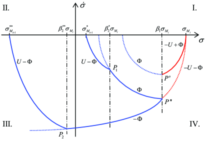
for a double-integrator with , the -trajectories can be calculated for an arbitrary initial state . Then, without loss of generality, consider the first extreme value , while the preceding reaching phase is always ensured by the initialization control (15). After applying first the control value , according to (14), the state trajectory proceeds in the IV-th quadrant, cf. Figure 2. While both limiting cases of the perturbation are effective, we focus here on the worst-case scenario, that is essential for convergence, in which the sign of is negative. Note that this renders the system to be underdamped. Using in the denominator of (16) and substituting the threshold value on the left-hand side of (16) one obtains the first peaking point (labeled by ) of the -state as
| (17) |
At this point, the control is switching from to . Then, evaluating the parabolic trajectory (16) between the and points, with and worst-case , one obtains
| (18) |
Substituting (17) into (18) and solving (18) with respect to results in
| (19) |
where the second peaking point is the one where the control is switching back from to . Continuing this line of calculations, one considers also the parabolic trajectory (16) after passing the -threshold as
| (20) |
Here again, is assumed as worst-case from a convergence point of view. Substituting the left-hand-side of (20) by the next extreme value , at which , results in
| (21) |
Note that for convergence, it is strictly required that
for all pairs of the consecutive extreme values, indexed by and . Since is guaranteed for all trajectories in the IV-th and III-rd quadrants, cf. Figure 2, the above convergence inequality can be written, with respect to (21), as
| (22) |
Substituting (19) into (22) yields
| (23) |
which results in the strict parameters condition
| (24) |
Furthermore, one needs to ensure
| (25) | |||||
| (26) |
in order to realize the both control switchings between two successive extreme values. Note that (25) is inherited from the conventional sub-optimal SMC, cf. (7). Here we emphasize that the parametric conditions (24), (25), (26) must be satisfied for the energy-saving sub-optimal SMC to yield the global convergence, for and irrespective the perturbations .
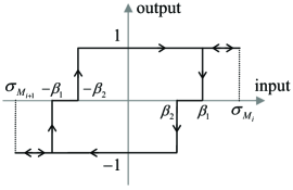
The imposed constraints (24), (25), (26) have an illustrative graphical interpretation as shown in Figure 1.
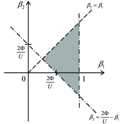
The values admissible for convergence are inside of a grey-shadowed triangle, while on the edge the energy-saving control (14), (15) reduces to the conventional sub-optimal SMC. Obviously, the ratio determines the size of an admissible set, including whether the negative -values are allowed. It is also worth noting that the opposite edge maximizes the distance. However, this can largely increase the convergence time (including ), similar as in case of a minimal-fuel control with free response time of an unperturbed double-integrator analyzed in detail in [8].
3.3 Reaching and convergence time
Consider first the reaching time between two consecutive extreme values and . Recall that a conservative approach is taken so that a worst-case scenario is calculated for all control phases, in terms of a slowest time. The associated trajectories of one reaching phase are schematically drawn in Figure 2. Similar as before, and without loss of generality, consider the first extreme value so that the trajectories proceed in the III-rd and IV-th quadrants. We recall that the threshold value can be either positive or negative, cf. Figure 1. Evaluating first the peaking point one obtains the corresponding -value as
| (27) |
which is reached by the slowest trajectory driven by . For the subsequent phase with control-off, i.e. , one needs distinguishing between two boundary trajectories, one driven by and another driven by . Also we notice that both control-off phases are considered starting from the same peaking point. Indeed, one can recognize that starting from , the -driven trajectory reaches the -abscissa later from than from peaking point, see Figure 2. For the control-off phase between the and thresholds, starting from and ending in peaking point, one obtains
| (28) |
Note that the second term under the square root in (28) must be positive, so here has to be larger than the point where the -driven trajectory reaches the -abscissa (see the dotted arc from in Figure 2).
With the determined values at all relevant peaking points, i.e. , , and , one can analyze the slowest time for each phase of a reaching cycle individually.
The slowest time of the first control-on phase is
| (29) |
In a similar way, one obtains the slowest time of the subsequent control-off phase driven by as
| (30) |
One can recognize that if (yielding the conventional sub-optimal SMC), then both square root terms in (30) become equal, and becomes zero. One can also recognize that the upper bound of is when the second square root term in (30) becomes zero. This results in the maximal control-off time of this phase equal to
| (31) |
When evaluating the control-off phase driven by , cf. Figure 2, we write
| (32) |
Substituting (17) and (19) into (32) and solving it with respect to results in
| (33) |
Here, it can also be recognized that has its maximal value when the second square root term in (33) becomes zero. Thus, the maximal control-off time for this phase is
| (34) |
Comparing both maximal time values, one can show that
holds always due to . Despite this fact, which determines the slowest control-off phase during one reaching cycle, we recall that the overall convergence time depends also on the number of cycles. Therefore, both (31) and (34) are taken into account in further calculations.
Evaluating both successive control-on phases, starting once from and once from peaking point, we obtain
| (35) |
and
| (36) |
respectively. Also here one can show, cf. (35), (36), that
holds always due to .
For analyzing the total worst-case (i.e. largest) reaching time between two consecutive extreme values and , one needs to distinguish between two pathes: and , cf. Figure 2. In the first case, the overall maximal reaching time is
| (37) |
In the second case, respectively, the overall maximal reaching time is
| (38) |
Note that in both above equations denote the terms where the control is off, i.e. , while denote the terms where the control is on, i.e. .
Once the convergence of the energy-saving sub-optimal SMC is guaranteed, being analyzed in Section 3.2, the overall accumulated worst-case reaching time results in
| (39) |
Because the convergence implies
| (40) |
the infinite sum in (39) turns out into a geometric series
| (41) |
which is convergent. This allows concluding that the upper bound of the finite time convergence is
| (42) |
Note that the initial reaching time of the first extreme value is , cf. (15). Furthermore, we note that depending on the branching of trajectories, as shown above for the control-off phase, also a maximum value must be taken into account in (42).
For determining and , we evaluate both subsequent extreme values and obtain, based on (16), the equations
| (43) |
and
| (44) |
Comparing (43) and (44) with (40), results in
| (45) |
and
| (46) |
Following the same line of calculations as above, one can evaluate the reaching and convergence time of the conventional sub-optimal SMC, for which . Considering the and peaking points results in
| (47) |
Then, the upper bound of the finite time convergence of the conventional sub-optimal SMC results in
| (48) |
where , cf. with (40). For evaluating , consider the peaking point and obtain
| (49) |
Note that both (45) and (46) reduce to (49) if assuming . Also worth noting is that (49) coincides with the convergence condition (24) if and requires
| (50) |
We will denote as amplification factors of the convergence time, and as contraction factors of the convergence. Inspecting (42) and (48), one can recognize that the former are proportionally increasing the convergence time while the latter can drastically slow down the overall convergence once become closer to one.
3.4 Energy-saving control parametrization
For the energy-saving sub-optimal SMC becomes effective, one needs to ensure that its total energy consumption is less than that of the conventional sub-optimal SMC, cf. condition (b) at the end of Section 2, while assuming the , , and values are the same. In terms of the both control-on phases, i.e. , the amplification factors to be taken into account are
| (51) |
and
| (52) |
cf. (37), (38). Taking out of consideration the initial reaching phase in (42) and (48), we obtain two energy cost functions
| (53) |
and
| (54) |
for the energy-saving and conventional sub-optimal SMC, respectively. In order to find an energy-saving pair of the threshold parameters for with some fixed process values satisfying , we formulate the
| (55) |
minimization problem under the hard constraint
| (56) |
In addition, in order to avoid , which can lead to , see [8] for details, we specify the upper bound
| (57) |
This implies restriction on the convergence time and, this way, forces a reasonable in course of solving the minimization problem (55).
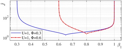
The convergence time cost function is exemplary visualized in Figure 3 in dependency of , for two cases assuming and . Note that for both boundary values , cf. (50), and .
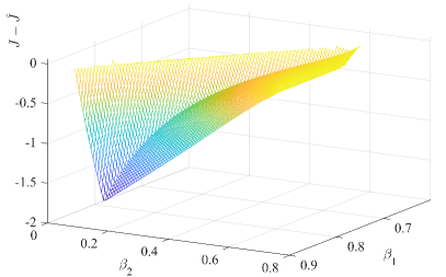
Note that the hard constraint (56) is required to ensure that the total control-on time of the energy-saving sub-optimal SMC is shorter than that of the conventional one. Moreover, one can recognize that (55) ensures the maximal possible energy-saving, due to the control-off phases throughout the convergence, comparing to the conventional sub-optimal SMC, both having the same value. That means for any fixed complying with (57), there is an optimal counterpart. The latter represents the solution of the constrained minimization problem (55). The results of the constrained optimization are exemplary visualized in Figure 4, for the perturbation to control ratio equal to .
It should be noted that the formulated optimization problem does not take explicitly into account those transient phases where the control is off, cf. (37), (38) and (51), (52). However, this does not imply any issues since the finite time convergence of the energy-saving sub-optimal SMC is upper bounded by (42).
4 Chattering due to actuator dynamics
If the system under control is subject to an additional (parasitic) actuator dynamics, the second-order sliding mode experiences the residual steady-state oscillations, also known as chattering, see e.g. [10, 11]. For the first-order actuator dynamics with a time constant , the control variable in (2) must be substituted by a new control variable , which is the solution of
Assume that the stable residual steady-state oscillations of the system (2) with the new input channel and control (14) are established. Then, the input-output map of the energy-saving sub-optimal SMC (14) takes the form of a three-state hysteresis relay as shown in Figure 5. For steady-state oscillations, the switching thresholds keep the constant values and are symmetric with respect to zero. Note that the amplitude of oscillations is determined by the cyclic extreme value . Furthermore, we note that if , the input-output map reduces to a standard two-state hysteresis relay, as it was used for harmonic balance analysis of the original sub-optimal control, cf. [12, chapter 5.2].
Before examining the residual oscillating behavior of the energy-saving sub-optimal SMC, recall the principle procedure of the describing function (DF) analysis, see e.g. [13], here in context of the second-order SMC and, in particular, when using the sub-optimal SMC. For the given DF of the SMC in feedback, denoted by , the harmonic balance equation
| (58) |
must have a real solution, in terms of the amplitude and angular frequency , for the residual steady-state oscillations to exist. Considering the double-integrator plant augmented by the first-order actuator dynamics, we write
| (59) |
For the conventional sub-optimal SMC, parameterized by and , the DF is given by, cf. [12],
| (60) |
Note that also for the generalized sub-optimal SMC, the DF analysis was provided in [14], cf. with (60). The negative reciprocal of (60) yields
| (61) |
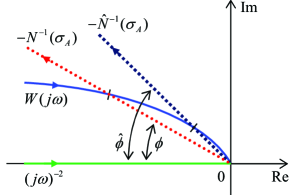
One can show that the locus of (61), that is its graphical interpretation in the harmonic balance (58), is a straight line starting in the origin and forming a clockwise angle , see Figure 6. The latter can be directly calculated as
| (62) |
One can recognize that larger -parameter values lead to a larger and, therefore, shirt the locus intersection towards higher frequencies and lower amplitudes.
Since the energy-saving sub-optimal SMC constitutes a linear combination of two negative hysteresis relays, cf. (14), its DF can be represented as a summation of two DFs of the type (60), this way resulting in
| (63) |
After evaluating the negative reciprocal of (63), similar to (61), we obtain
| (64) |
In Figure 6, the negative reciprocal of both DFs are depicted, once of the conventional sub-optimal SMC with DF (60) and once of the energy-saving sub-optimal SMC with DF (63), together with the Nyquist plots of and double integrator . The energy-saving sub-optimal SMC has always a lower angle for the same fixed value, while for the angle . One can also recognize that unlike the double integrator, the Nyquist plot of has always an intersection point with the negative reciprocals of DFs. This implies an existence of solutions of the harmonic balance equation (58). The corresponding steady-state oscillations have a higher amplitude and lower frequency for the energy-saving sub-optimal SMC compared to those of the conventional sub-optimal SMC.
5 Numerical examples
This section demonstrates the numerical examples which characterize the main properties of the energy-saving sub-optimal SMC formulated and analyzed above. Implemented is a double-integrator system (2) with and the energy-saving sub-optimal SMC (14). For simulating the conventional sub-optimal SMC, the threshold value is set , cf. section 2. All simulation results are obtained by using the simple first-order Euler-type numerical solver with the fixed-step size of 0.001 sec.
5.1 Convergence behavior
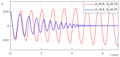
The convergence behavior of the energy-saving sub-optimal SMC is exemplary shown for examining the parametric condition (24). The constraining parameters are chosen so that with and , while for a worst-case scenario of the bounded perturbation is assumed. Note that the assumed constitutes an always ’co-acting’ perturbation signal of the maximal amplitude , a worst-case scenario that challenges the contraction during each reaching cycle and, at large, the total convergence to equilibrium. Figure 7 discloses the converging behavior for , versus the diverging behavior for , . Note that here, the threshold values distance is required for (24) is fulfilled.
5.2 Energy-saving versus conventional sub-optimal SMC
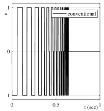
The energy-saving sub-optimal control behavior is analyzed in comparison to the conventional sub-optimal one, with regard to the recorded convergence time and overall energy consumption
In order to determine the numerical convergence instant, the value is obtained once the Euclidian norm of the state vector decreases below some assigned low residual constant, i.e. . The residual constant is determined out from the numerical simulations, with respect to the solver type and step-size and the resulted numerical pattern around after the principal dynamics of has converged. For the assigned ratio with and , three configurations of the perturbing signal are considered: , , . Note that the second one is ’co-acting’ to the control signal. This has, however, an adverse impact on contraction of the state trajectories, cf. Figure 2. The third one acts, on the contrary, as a maximal possible system damping and can negatively affect the control-off phases in terms of the reaching time, cf. section 3.3. Two parameter sets, obtained from the constrained optimization, and cf. with Figure 4, are used. All simulation results are summarized in Table 1. Recall that for the conventional sub-optimal SMC the is always assigned.
| , | , | |||
|---|---|---|---|---|
| Configuration | ||||
|
conventional
|
0.420 | 0.391 | 0.643 | 0.580 |
|
energy-saving
|
0.345 | 0.292 | 0.332 | 0.176 |
|
conventional
|
0.342 | 0.285 | 0.552 | 0.448 |
|
energy-saving
|
0.288 | 0.247 | 0.435 | 0.278 |
|
conventional
|
0.517 | 0.441 | 0.645 | 0.548 |
|
energy-saving
|
0.442 | 0.325 | 3.718 | 0.155 |
One can recognize a superior performance of the energy-saving sub-optimal SMC in all above given cases, except the last row in Table 1 (see light red shadowed). Here the energy saving is largely achieved, but the convergence time is significantly increased comparing to the conventional sub-optimal SMC. This is related to a relatively slowly ’drifting’ trajectory between the lying apart and , being driven by the perturbation. The situation with improves, still guaranteing for energy saving, when both threshold parameters are lying closer to each other like in the shown case and , see Table 1.
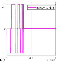
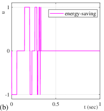
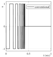
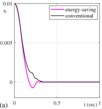
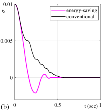
For better interpreting the listed results, some of the above configurations are shown below in the plots of and . All configurations with are depicted in Figures 8 and 9.
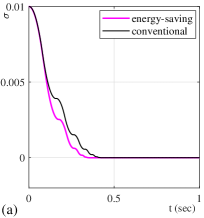
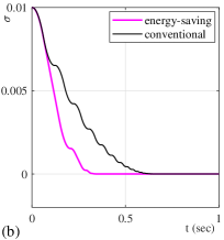
One can see that the energy-saving sub-optimal SMC converges faster, correspondingly stops to switch earlier than its conventional counterpart. One can also notice that both controllers here disclose a monotonic convergence without twisting, cf. section 2.
The convergence in case of is also exemplary shown in Figure 10. Here, the conventional sub-optimal SMC has a monotonic convergence, in accord with (13). On the contrary, the energy-saving sub-optimal SMC changes into twisting mode here, because it allows for control phases driven only by the perturbation quantity.
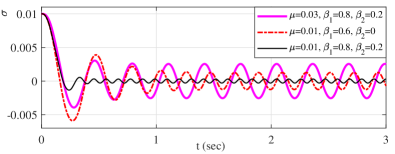
5.3 Residual steady-state oscillations
For evaluating the residual oscillations (i.e. chattering) owing to a parasitic actuator dynamics, cf. section 4, different parameter sets with are compared. Three parameter configurations used are shown in Table 2. The amplitude and frequency of the residual steady-state oscillations are computed based on the harmonic balance analysis provided in section 4, i.e. using (65), (66), and compared with those out from the numerical simulations. Certain, yet acceptable, error of the harmonic balance analysis is not surprising, since DF solely approximates the first main harmonic, cf. with results in [14].
| Harmonic balance | Numerical simulation | |||
|---|---|---|---|---|
| Parameters | ||||
| , , | 0.0019 | 21.1 | 0.0025 | 20.0 |
| , , | 0.00085 | 33.3 | 0.0012 | 30.2 |
| , , | 0.00021 | 63.3 | 0.00029 | 59.3 |
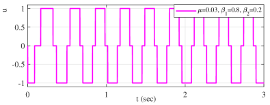
Figure 11 exemplifies the appearance of residual steady-state oscillations when the actuator dynamics is in place. The time response of the sliding variable is shown above for all three parameter sets, cf. Table 2. The control value , i.e. of the control (14), is exemplary shown below for the parameter set , , .
6 Conclusions
The problem of saving energy by the control-off phases in the second-order sliding modes was addressed. More specifically, the conventional sub-optimal SMC, see [7] for survey, was extended for a class of the systems (2) with and . This way, a well parameterizable phase appears within each reaching cycle, during the entire finite-time convergence. The latter was estimated for the worst-case scenario of an upper-bounded perturbation occurring in each control phase. The analyzed contraction and maximal reaching- as well as total convergence-time served to formulate a constrained minimization problem for an energy cost function. Two switching threshold parameters represent the solution of a complex nonlinear optimization, while the perturbation-boundary to control-authority ratio, i.e. , is crucial for convergence and energy-saving conditions. Also the impact of an additional parasitic actuator dynamics, typical for real sliding modes in terms of chattering, was analyzed based on the harmonic balance. The overall analysis performed and the dedicated numerical evaluations argue in favor of using the proposed energy-saving sub-optimal SMC for . In applications, a resettable control-off mode can also be added for , this way ensuring energy saving after convergence and a reactivation in case of perturbations in the equilibrium.
References
- [1] V. Utkin, Sliding modes in control and optimization, Springer, 1992.
- [2] C. Edwards, S. Spurgeon, Sliding mode control: theory and applications, CRC Press, 1998.
- [3] Y. Shtessel, C. Edwards, L. Fridman, A. Levant, Sliding mode control and observation, Springer, 2014.
- [4] A. Levant, Sliding order and sliding accuracy in sliding mode control, Inter. Journal of Control 58 (6) (1993) 1247–1263.
- [5] L. Fridman, A. Levant, Higher order sliding modes, Marcel Dekker New York, 2002, pp. 53–102.
- [6] G. Bartolini, A. Ferrara, E. Usai, Output tracking control of uncertain nonlinear second-order systems, Automatica 33 (12) (1997) 2203–2212.
- [7] G. Bartolini, A. Pisano, E. Punta, E. Usai, A survey of applications of second-order sliding mode control to mechanical systems, Inter. Journal of Control 76 (9–10) (2003) 875–892.
- [8] M. Athans, Fuel-optimal control of a double integral plant with response time constraints, IEEE Transactions on Applications and Industry 83 (73) (1964) 240–246.
- [9] G. Bartolini, A. Ferrara, A. Levant, E. Usai, On second order sliding mode controllers, Springer, 1999, pp. 329–350.
- [10] G. Bartolini, A. Ferrara, E. Usai, Chattering avoidance by second-order sliding mode control, IEEE Transactions on Automatic Control 43 (2) (1998) 241–246.
- [11] I. Boiko, L. Fridman, A. Pisano, E. Usai, Analysis of chattering in systems with second-order sliding modes, IEEE Transactions on Automatic Control 52 (11) (2007) 2085–2102.
- [12] I. Boiko, Discontinuous control systems: frequency-domain analysis and design, Birkhaeuser, 2009.
- [13] D. Atherton, Nonlinear Control Engineering - Describing Function Analysis and Design, Workingam Beks, 1975.
- [14] I. Boiko, L. Fridman, R. Iriarte, A. Pisano, E. Usai, Parameter tuning of second-order sliding mode controllers for linear plants with dynamic actuators, Automatica 42 (5) (2006) 833–839.