Energy Harvesting in Unmanned Aerial Vehicle Networks with 3D Antenna Radiation Patterns
Abstract
In this paper, an analytical framework is provided to analyze the energy coverage performance of unmanned aerial vehicle (UAV) energy harvesting networks with clustered user equipments (UEs). Locations of UEs are modeled as a Poisson Cluster Process (PCP), and UAVs are assumed to be located at a certain height above the center of user clusters. Hence, user-centric UAV deployments are addressed. Two different models are considered for the line-of-sight (LOS) probability function to compare their effects on the network performance. Moreover, antennas with doughnut-shaped radiation patterns are employed at both UAVs and UEs, and the impact of practical 3D antenna radiation patterns on the network performance is also investigated. Initially, the path loss of each tier is statistically described by deriving the complementary cumulative distribution function and probability density function. Following this, association probabilities with each tier are determined, and energy coverage probability of the UAV network is characterized in terms of key system and network parameters for UAV deployments both at a single height level and more generally at multiple heights. Through numerical results, we have shown that cluster size and UAV height play crucial roles on the energy coverage performance. Furthermore, energy coverage probability is significantly affected by the antenna orientation and number of UAVs in the network.
Index Terms:
Unmanned aerial vehicles (UAVs), energy harvesting, energy coverage probability, Poisson point processes, Poisson cluster processes, Thomas cluster processes, 3D antenna radiation patterns, stochastic geometry.I Introduction
To support the unprecedented growth in demand for mobile data fueled by emerging wireless applications and the increased use of smart mobile devices, new technologies and designs are being incorporated into next-generation cellular networks. One novelty is expected to be the deployment of unmanned aerial vehicle (UAV) base stations (BSs). UAVs have been primarily considered as high-altitude platforms at altitudes of kilometers to provide coverage in rural areas. On the other hand, use of low-altitude UAVs has also become popular recently due to the advantage of having better link quality in shorter-distance line-of-sight (LOS) channels with the ground users. Moreover, owing to the relative flexibility in UAV deployments, UAV BSs can be employed in a variety of scenarios including public safety communications and data collection in Internet of Things (IoT) applications [1], [2]. Other scenarios include disasters, accidents, and other emergencies and also temporary events requiring substantial network resources in the short-term such as in concerts and sporting events. In such cases, UAVs can be deployed rapidly to provide seamless wireless connectivity [3]–[5].
In addition to growing data traffic, increasing number of devices results in a significant growth in energy demand. RF (radio frequency) energy harvesting where a harvesting device may extract energy from the incident RF signals has emerged as a promising solution to power up low-power consuming devices [6], [7]. Therefore, the advances in energy harvesting technologies have motivated research in the study of different wireless energy harvesting networks. For example, wireless energy and/or information transfer in large-scale millimeter-wave and microwave networks has been studied in [8]–[11]. In these works, energy is harvested wirelessly from energy transmitters which are generally deployed at fixed locations. However, low-power consuming devices can potentially be distributed in a large area. In such cases, the performance of energy harvesting will be limited by the low end-to-end power transmission efficiency due to the loss of RF signals over long distances [12].
In order to improve the efficiency, instead of fixed energy transmitters such as ground base stations (BSs), the deployment of mobile energy transmitters is proposed recently. In particular, although the UAVs are typically power-limited, UAV-assisted energy harvesting has become attractive due to the flexibility and relative ease in deploying UAV BSs. In [13], mobility of the UAV with a directional antenna is exploited by jointly optimizing the altitude, trajectory, and transmit beamwidth of the UAV in order to maximize the energy transferred to two energy receivers over a finite charging period. In [12], authors consider a more general scenario with more than two energy receivers where the amount of received energy by all energy receivers is maximized via trajectory control. In [14], a UAV-enabled wireless power transfer network is studied as well. Minimum received energy among all ground nodes is maximized by optimizing the UAV’s one-dimensional trajectory. Both downlink wireless power transfer and uplink information transfer is considered in [15] with one UAV and a set of ground users. The UAV charges the users in downlink and users use the harvested energy to send the information to the UAV in the uplink. Similarly, a wireless-powered communication network with a mobile hybrid access point UAV is considered in [16]. In this work, the UAV performs weighted energy transfer and receives information from the far-apart nodes based on the weighted harvest-then-transmit protocol. The use of UAVs to power up energy constrained sensor nodes has been suggested in [17]. UAVs are considered to be equipped with the dedicated chargers facing the ground so that they can recharge the sensors’ batteries using RF energy harvesting. A practical example is AT&T’s flying Cell on Wings (COW) drones [18]. In particular, AT&T’s COW is a UAV equipped with a small base station. Flying COW is tethered to a power source on the ground with a cable. In these types of practical implementations, power constraints are more relaxed and such a UAV can provide both cell service and also supply wireless energy to sensors and small IoT devices.
In a separate line of research in the literature, the performance of UAV-assisted wireless networks is extensively studied recently. Similar to 2D networks, stochastic geometry has been employed in the network level analysis of UAV networks by considering UAVs distributed randomly in 3D space. Effect of different network parameters on the coverage probability is explored in several recent works such as [19]–[23]. In [24], authors analyzed the network performance for three different type of LOS probability models. Spectrum sharing in UAV networks is analyzed in [25]–[27]. Additionally, optimal deployment of UAVs is investigated in [28]–[30].
It is important to note that the antenna number, type, and orientation are critical factors that affect the performance in UAV-assisted networks. Indeed, several recent studies, e.g., [31] and [32], have addressed scenarios in which antenna arrays are deployed in UAV-assisted cellular networks. Similarly, in [33], the authors have considered directional antennas for UAVs. However, a practical antenna pattern which is omnidirectional in the horizontal plane but directional in the vertical plane is employed for ground BSs. Regarding the antenna type, omnidirectional antennas can also be used in UAVs, especially considering their mobility [34]. At the same time, since even the UAV’s own body can shadow the antenna and result in a poor link quality, the orientation of the antennas plays an important role on the performance [35]. There has been limited analytical and experimental works studying the effect of three dimensional (3D) antenna radiation patterns on the link quality between the UAV and ground users. In [35], impact of antenna orientation is investigated by placing two antennas on a fixed wing UAV flying on a linear path with 802.11a interface. Similarly, path loss and small-scale fading characteristics of UAV-to-ground user links are analyzed with a simple antenna extension to 802.11 devices in [36]. In [37], ultra-wideband (UWB) antennas with doughnut-shaped radiation patterns are employed at both UAVs and ground users to analyze the link quality at different link distances, UAV heights, and antenna orientations. The large bandwidth of UWB radio signals is utilized in the measurements to obtain a high temporal resolution of multipath components. Authors develop a simple analytical model to approximate the impact of the 3D antenna radiation pattern on the received signal. However, none of these works study the effect of UAV antenna orientation on the network performance.
I-A Contributions and Organization
In this paper, we consider a UAV network consisting of UAVs operating at a certain altitude above ground. The locations of user equipments (UEs) are modeled as a Poisson cluster process (PCP), and the UAVs are assumed to be located at a certain height above the center of user clusters. Since UAVs are deployed in overloaded scenarios, locations of UAVs and UEs are expected to be correlated and UEs are more likely to form clusters. Hence, modeling the UE locations by PCP is more appropriate and realistic. Moreover, we consider that UWB antennas with doughnut-shaped radiation patterns are employed at both UAVs and UEs, and we study the effect of practical 3D antenna radiation patterns on energy harvesting from UAVs.
More specifically, our main contributions can be summarized as follows:
-
•
An analytical framework is provided to analyze energy coverage performance of a UAV network with clustered UEs. UE locations are assumed to be PCP distributed to capture the correlations between the UAV and UE locations.
-
•
We divide the network into two tiers: tier UAV and tier UAVs. tier UAV is the cluster center UAV around which the typical UE is located, while other UAVs constitute the tier.
-
•
Two different LOS probability functions, i.e., a high-altitude model and a low-altitude model, are considered in order to investigate and compare their impact on the network performance.
-
•
Different from the previous studies, more practical antennas with doughnut-shaped radiation patterns are employed at both UAVs and UEs to provide a more realistic performance evaluation for the network.
-
•
We first derive the complementary cumulative distribution functions (CCDFs) and the probability density functions (PDFs) of the path losses for each tier, then obtain the association probabilities by using the averaged received power UAV association rule.
-
•
Average harvested power expression is obtained. Then, total energy coverage probability is determined by deriving the Laplace transforms of the interference terms arising from each tier. Energy coverage is characterized for UAV deployments at a single height level and also at multiple heights.
The rest of the paper is organized as follows. In Section II, system model is introduced, and path loss, blockage, and 3D antenna models are described. Path loss and association probabilities are statistically characterized in Section III. In Section IV, energy coverage probability of the UAV network is determined. In Section VI, simulations and numerical results are provided, demonstrating the impact of several key parameters on the energy coverage performance of the network. Finally, Section VII concludes the paper. Proofs are included in the Appendix.
II System Model
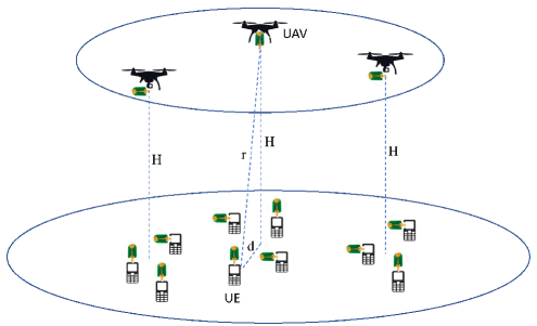
In this section, we describe the system model of the UAV network with clustered UEs. We address a downlink network, in which the spatial distribution of the UAVs is modeled by an independent homogeneous PPP with density on the Euclidean plane. The height of UAVs is denoted by . Note that UAVs can be used to offload traffic from the ground cellular BSs and reduce congestion around hotspots. In energy harvesting applications, UAVs can be used to transfer energy to e.g., ground sensors and low-power IoT devices, to energize them. They can also be deployed in case of emergencies during which ground infrastructure is strained [38]. In our model, the UEs are clustered around the projections of UAVs on the ground, and the locations of the clustered UEs is described by a PCP, denoted by . In applications involving UAVs, UEs are expected to be located in high UE density areas, forming clusters. Consequently, modeling of UE distribution as a PCP rather than a homogeneous PPP is more accurate.
In this paper, we model as a Thomas cluster process, where the UEs are symmetrically independently and identically distributed (i.i.d.) around the cluster centers (which are projections of UAVs on the ground), according to a Gaussian distribution with zero mean and variance . Therefore, the UE’s location is statistically described by the following PDF and CCDF [39]:
| (1) | ||||
| (2) |
respectively, where is the 2D distance of a UE with respect to the cluster center on the ground. Without loss of generality, we perform the analysis for a typical UE which is randomly chosen from a randomly chosen cluster. Since cluster centers; i.e. UAVs, are PPP distributed and the PPP is stationary, location of this typical UE can be transformed to the origin according to Slivnyak’s theorem [40]. The typical UE is assumed to be is associated with the UAV providing the maximum average received power. Although we have only a single-tier network composed of UAVs, we also consider an additional tier, named as tier that only includes the cluster center of the typical UE similarly as in [21] and [40]. Therefore, overall UAV density is equal to tier 1 density, and tier 0 has only one UAV, which is the cluster center of the typical UE. Essentially tier 0 is introduced to differentiate the cluster-center UAV from other UAVs, because the distance distribution equations of the typical UE to its own cluster-center UAV given in (1) and (2) are different from the distribution of the distances to other UAVs. Thus, our network model can be considered as a two-tier network consisting of a tier cluster-center UAV and tier UAVs. The considered network model is depicted in Fig. 1.
II-A Path Loss and Blockage Modeling
A transmitting UAV can either have a line-of-sight (LOS) or non-line-of-sight (NLOS) link to the typical UE. Consider an arbitrary link of length between a UE and a UAV, and define the LOS probability function as the probability that the link is LOS. Different LOS probability functions have been used in the literature. In this paper, we consider the two models proposed in [41] and [42], which are high-altitude and low-altitude models, respectively.
High-altitude model is widely used especially in satellite communications where the altitude is around hundred of kilometers. It has also been widely employed in UAV-assisted networks recently. LOS probability function for the high-altitude model is given as follows:
| (3) |
where is the 3D distance between the UE and UAV, is the UAV height, and are constants whose values depend on the environment. It can be easily verified that the LOS probability in (3) increases as the UAV height, , increases.
Since practical values for UAV height in certain applications is around meters, a more realistic LOS probability function proposed for 3GPP terrestrial communications is employed also for UAV networks in [24]. The height of a macrocell base station is usually around 32 m, which is comparable to the practical UAV height. Therefore, employment of the LOS probability function for 3GPP macrocell-to-UE communciation is also reasonable for the UAV networks in such relatively low-altitude scenarios. For the low-altitude model, LOS probability function is expressed as
| (4) |
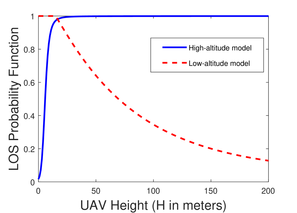
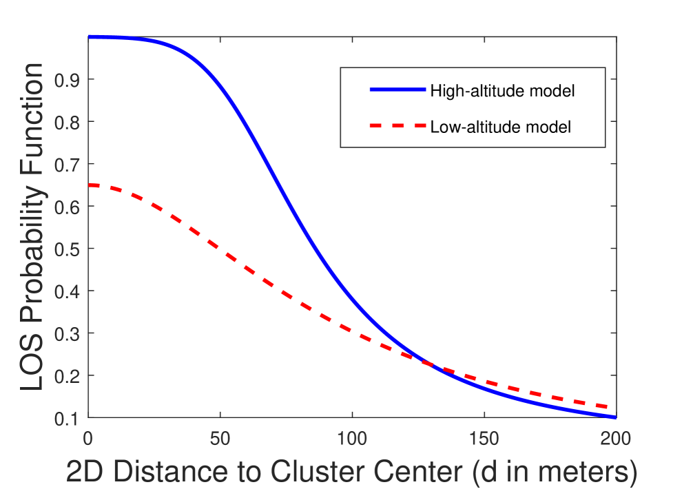
Note that different from the high-altitude model, LOS probability function in (4) decreases with the increase in the 3D distance , independent of the UAV height. In Fig. 2, LOS probability function is plotted using high-altitude and low-altitude models. Solid lines show the LOS probability as a function of the UAV height when the 2D distance to the UAV is fixed at m, and dashed lines display the LOS probability as a function of the 2D distance to the UAV when the UAV height is m. As shown in Fig. 2, LOS probability increases with increasing UAV height when the high-altitude model is used, and decreases when the low-altitude model is considered. We observe that the LOS probability decreases for both models as the 2D distance to the UAV increases. We also note that the analysis in the remainder of the paper is general and is applicable to any LOS probability function. Only in Section VI, we employ the LOS probability functions in (3) and (4) to obtain the numerical results.
In general, NLOS links experience higher path loss than the LOS links due to signals being reflected and scattered in NLOS propagation environments. Therefore, different path loss laws are applied to LOS and NLOS links. Thus, the path loss on each link in tier can be expressed as
| (5) |
where and are the LOS and NLOS path-loss exponents, respectively.
II-B 3D Antenna Modeling
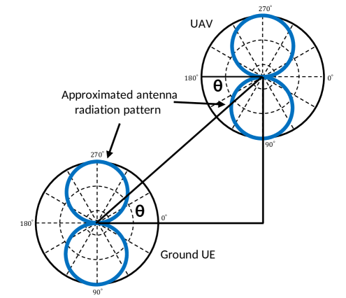
In this paper, we consider the analytical model developed in [37] for the effect of 3D antenna radiation patterns on the received signal. UWB transmitter and receiver antennas with doughnut-shaped radiation patterns centered at a frequency of 4 GHz are placed at the UAV and UE, respectively, and air-to-ground channel measurements are carried out in order to characterize the impact of the 3D antenna radiation pattern on the received signal for different antenna orientations in [37]. As a result of these measurements, transmitter and receiver antenna gains are modeled analytically for horizontal-horizontal (HH), horizontal-vertical (HV) and vertical-vertical (VV) antenna orientations as follows:
| (6) |
where is the elevation angle between the transmitter at the UAV and the receiver at the UE on the ground. In this antenna model, radiation pattern is approximated by a circle in the vertical dimension, while it is assumed to be constant for all horizontal directions. In other words, antenna gains depend only on the elevation angle , and are considered as independent of the azimuth angle between the transmitter at the UAV and the receiver at the UE. Approximated antenna radiation patterns of UAV and UE are shown in Fig. 3 for HH antenna orientation. They can be plotted for HV and VV orientations as well by rotating the transmitter and/or receiver antennas by . Note that for HH antenna orientation as which happens when the UEs are located far away from the cluster center, i.e. as the increases, and as which happens when the UEs get closer to the cluster center. Similar observations can be drawn for VH and VV antenna orientations. Effective antenna gain as a function of can be rewritten in terms of UAV height and the path loss on each link in tier as
| (7) |
In the rest of the analysis, we assume that the typical UE and all UAVs in the network have horizontal antenna orientation. Therefore, HH antenna orientation for the main link and interfering links are considered due to its analytical tractability. Moreover, UEs are considered to be clustered around the projections of UAVs on the ground and more UEs are encouraged to be associated with their cluster center UAV. As a result, the angle between the transmitter at the UAV and the receiver at the UE is expected to be large. Therefore, HH antenna orientation is more suitable than the other two orientations. However, in the numerical results section, simulation results for HV and VV orientations are also provided in order to compare their effect on the UAV association and energy coverage probabilities.
Finally, we note that a summary of notations is provided in Table I below.
| Notations | Description |
| PPP of UAVs, the density of , PCP of UEs. | |
| Height of UAVs. | |
| UE distribution’s standard deviation. | |
| 2D distance of a UE with respect to the cluster center on the ground. | |
| 3D distance between the UE and UAV. | |
| LOS probability functions for high and low altitude models. | |
| Environment dependent constants. | |
| Path losses on LOS and NLOS links in the tier. | |
| LOS and NLOS path-loss exponents. | |
| Transmitter and receiver antenna gains. | |
| Effective antenna gain. | |
| Elevation angle between the transmitter and the receiver. | |
| CCDF of the path loss from a typical UE to a tier UAV. | |
| PDF of the path loss from a typical UE to a tier LOS/NLOS UAV. | |
| Transmit power of UAVs in the tier. | |
| Small-scale fading gain. | |
| Association probability with a tier LOS/NLOS UAV. | |
| Interference from the tier UAV, when the main link is in the tier. | |
| Exclusion disc of path loss, inside which no interference exists. | |
| Total received power | |
| Conditional energy coverage probability given that the UE is associated with a tier LOS/NLOS UAV. | |
| Energy outage threshold. | |
| Rectifier efficiency. | |
| Laplace transform of . |
III Path Loss and UAV Association
III-A Statistics of the Path Loss
In this section, we provide statistical characterizations by identifying the CCDF and the PDF of the path loss.
Lemma 1: The CCDF of the path loss from a typical UE to a tier UAV can be formulated as
| (8) |
where is given in (1), and is the LOS or NLOS probability depending on whether or 111For instance, LOS probability is given by (3) and (4) for the high-altitude and low-altitude models, respectively, and NLOS probability is ..
Proof: See Appendix -A.
Lemma 2: CCDF of the path loss from a typical UE to a tier UAV is
| (9) |
where is given by
| (10) |
Proof: See Appendix -B.
Corollary 1: The PDF of the path loss from a typical UE to a tier LOS/NLOS UAV can be determined by applying the Leibniz integral rule as follows:
| (11) |
Corollary 2: The PDF of the path loss from a typical UE to a tier LOS/NLOS UAV is
| (12) |
where is given by
| (13) |
by again applying the Leibniz integral rule.
In the results above, we have determined the CCDFs and PDFs of the path loss for each tier. They depend on the key network parameters including the variance of the cluster process , UAV density , UAV LOS probability , UAV height and path loss exponents . In the following sections, these distributions are utilized in determining the association and energy coverage probabilities.
III-B UAV Association
In this work, we assume that the UEs are associated with a UAV providing the strongest long-term averaged power. In other words, a typical UE is associated with its cluster center UAV, i.e., the tier UAV, if
| (14) |
where and denote the transmit power and antenna gain of the link, respectively, in tier . is the path loss from the tier UAV, and is the path loss from tier UAV providing the minimum path loss. In the following lemma, we provide the association probabilities using the result of Lemmas 1, Lemma 2, Corollary 1 and Corollary 2.
Lemma 3: The association probabilities with a tier LOS/NLOS UAV and tier LOS/NLOS UAV are given, respectively, as
| (15) |
| (16) |
where and .
Proof: See Appendix -C.
In the corollary below, we provide a closed-form expression for the association probability in a special case with which the effects of different parameters on association probability can be easily identified.
Corollary 3: Consider the same UAV network with and the LOS probability , i.e., all UAVs are LOS to the typical UE. Then, the association probabilities specialize to the following expressions (which also confirm the results in [43]):
| (17) | ||||
| (18) |
with . According to the these results, a typical UE obviously prefers to connect to the tier UAV when the value of is small, and connect to a tier UAV for higher values of and .
IV Energy Coverage Probability Analysis
In this section, we use stochastic geometry and adopt an analytical framework to characterize the energy coverage probability for a typical UE clustered around the tier UAV (i.e., its own cluster-center UAV).
IV-A Downlink Power Transfer
The total power received at a typical UE at a random distance from its associated UAV in the tier can be written as
| (19) |
where the received power from the serving UAV and the interference power received from the UAVs in the tier are given as follows:
| (20) | ||||
| (21) | ||||
| (22) |
where and are the small-scale fading gains from the serving and interfering UAVs, respectively. Note that since only one UAV exists in the tier, . denotes the small-scale fading gain and is assumed to be exponentially distributed. From the UAV association policy, when a typical UE is associated with a UAV whose path loss is , there exists no UAV within a disc centered at the origin, which is also known as the exclusion disc. In this work, we also consider a linear energy harvesting model in which energy can be harvested if the received power is larger than zero. Therefore, the average harvested power at a typical UE is given in the following theorem.
Lemma 4: The average harvested power at a typical UE at a random distance from its associated UAV in the tier is given at the top of the next page in (23)
| (23) |
where
| (24) |
| (25) |
Proof: See Appendix -D.
IV-B Energy Coverage Probability
The energy harvested at a typical UE in unit time is expressed as where is the rectifier efficiency, and is the total received power given in (19). Since the effect of additive noise power is negligibly small relative to the total received power, it is omitted [8]. The conditional energy coverage probability is the probability that the harvested energy is larger than the energy outage threshold given that the typical UE is associated with a UAV from the tier, i.e., . Therefore, total energy coverage probability for the typical UE can be formulated as
| (26) |
where is the conditional energy coverage probability given that the UE is associated with a tier LOS/NLOS UAV, and denotes the association probability. The following theorem provides our main characterization regarding the total energy coverage probability.
Theorem 1.
In a UAV network with practical HH antenna radiation patterns and clustered UEs, the total energy coverage probability for the typical UE is approximately given at the top of the next page in (27)
| (27) |
where , , is the number of terms in the approximation and the Laplace transforms of the interference terms are given by
| (28) |
| (29) |
Proof: See Appendix -E.
Note that since tier consists of only one UAV, i.e., the cluster center UAV, Laplace transform expression . The total energy coverage probability of the network in Theorem 1 is obtained by first computing the conditional energy coverage probability given that a UE is associated with a tier LOS/NLOS UAV, and then summing up the conditional probabilities weighted with their corresponding association probabilities. In order to formulate the conditional energy coverage probabilities, Laplace transforms of the interference terms are determined. We also note that although the energy coverage probability approximation in Theorem 1 involves multiple integrals, we explicitly see the dependence of the energy coverage on, for instance, UAV heights, path loss distributions, path loss exponents, transmission power levels. Moreover, the integrals can be readily computed via numerical integration methods, providing us with additional insight on the impact of key system/network parameters, as demonstrated in the next section.
V Extension to a Model with UAVs at Different Heights
In the preceding analysis, we analyzed the energy coverage performance of a network in which UAVs are located at a height of above the ground, and is assumed to be the same for all UAVs. However, the proposed analytical framework can also be employed to analyze the coverage probability when UAV height is not fixed, i.e., UAVs are assumed to be located at different heights. In the extended model, we consider a more general network in which UAVs are located at different heights. Therefore, we assume that there are groups of UAVs such that the UAV group is located at the height level for and UAVs at each height level can be considered as a UAV-tier distributed according to an independent homogeneous PPP with density of and the total density is equal to . Different from the preceding analysis in which we have considered a single typical UE located at the origin and named its cluster center UAV as tier UAV, a separate typical UE for each UAV tier needs to be considered in the coverage probability analysis for this model with UAVs at different heights. For example, when we are analyzing the energy coverage probability of the network for a UE clustered around a tier UAV, we assume that the typical UE is located at the origin and its cluster center UAV is considered as the tier UAV similar to the previous model. Therefore, total energy coverage probability of the network given that the typical UE is clustered around a tier UAV for can be computed as follows:
| (30) |
where is the conditional energy coverage probability given that the typical UE is clustered around a tier UAV and it is associated with a tier LOS/NLOS UAV, and is the association probability with a tier LOS/NLOS UAV.
Theorem 2.
In a UAV network with practical HH antenna radiation patterns and clustered UEs, the total energy coverage probability of the network given that the typical UE is clustered around a tier UAV is approximately given at the top of the next page in (31)
| (31) |
Proof: Derivation of follows similar steps as that of in (27). In particular, Laplace transforms and for are computed using the Laplace transform equations given in (28) and (29), respectively, by updating UAV height as and UAV density as for . and are computed using (8) and (11), respectively, by denoting the UAV height as . Furthermore, and are computed using (9) and (12), respectively, by updating UAV height as and UAV density as for .
VI Simulation and Numerical Results
In this section, we present the numerical evaluations of theoretical expressions in addition to the simulation results which are provided to confirm the accuracy of the proposed UAV network model and the analytical characterizations. In the numerical computations and simulations, unless stated otherwise, the parameter values listed in Table II are used.
| Description | Parameter | Value |
| Path-loss exponents | , | 2, 4 |
| Environment dependent constants | , | , |
| Height of UAVs | m | |
| Transmit power | 37 dBm | |
| Energy outage threshold | 0 dBm | |
| UAV density | ||
| UE distribution’s standard deviation | 10 | |
| Rectifier efficiency | 1 |
VI-A Impact of Cluster Size
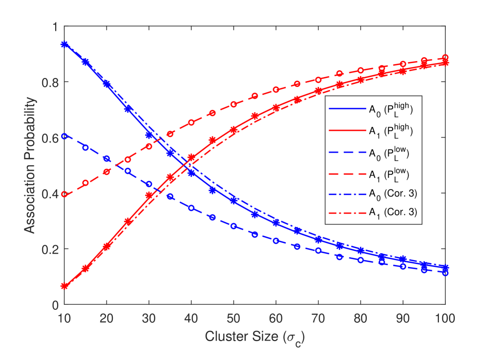
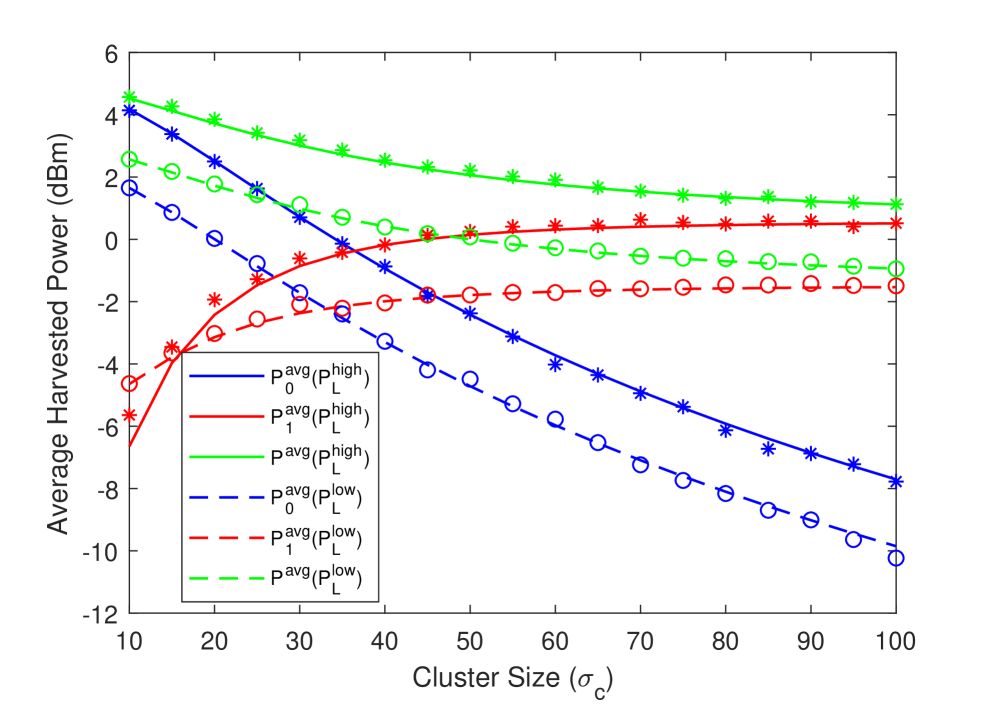
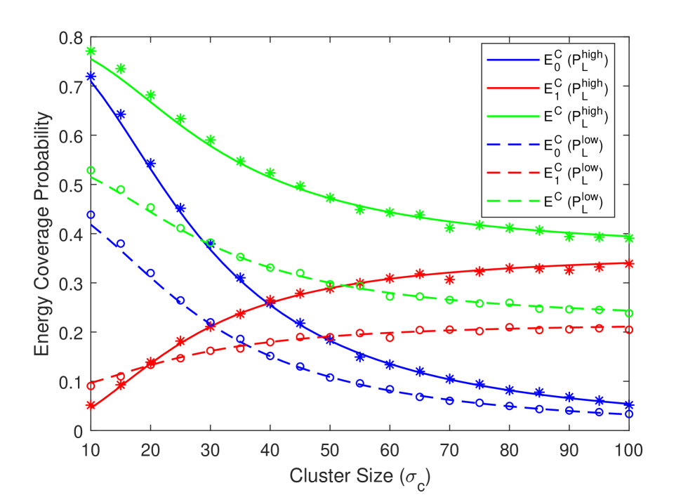
First, we address the effect of UE distribution’s standard deviation on the association probability, average harvested power and the energy coverage probability using the LOS probability functions of high-altitude and low-altitude models of (3) and (4) in Figs. 4(a), 4(b) and 4(c). As the standard deviation increases, the UEs are spread more widely, resulting in generally larger distances between the cluster-center tier UAV and UEs. For example, for , the average link distance between cluster center UAV and UEs is around 12.5 meters, while it is around 115 meters for . Consequently, association probability with the tier UAV, , diminishes, while the association probability with tier UAVs, , increases for both models. Also, for a fixed height, LOS probability of cluster center UAV decreases for both models with the increasing cluster size, and hence association probabilities exhibit similar trends. Therefore, the average harvested power from the tier UAV, , increases while the average harvested power from the tier UAVs, , decreases as the cluster size grows in both models. On the other hand, the increase in cannot compensate the decrease in , and therefore the total average harvested power diminishes. In other words, smaller cluster size, i.e., more compactly distributed UEs results in a higher . The energy coverage probability in Fig. 4(c) exhibits a very similar behavior as the average harvested power in Fig. 4(b). Also note that, the association probability results of the Corollary 3 closely approximate the association probabilities of the high-altitude model. Finally, we note that simulation results are also plotted in the figure with markers and there is generally an excellent agreement with the analytical results, further validating our analysis.
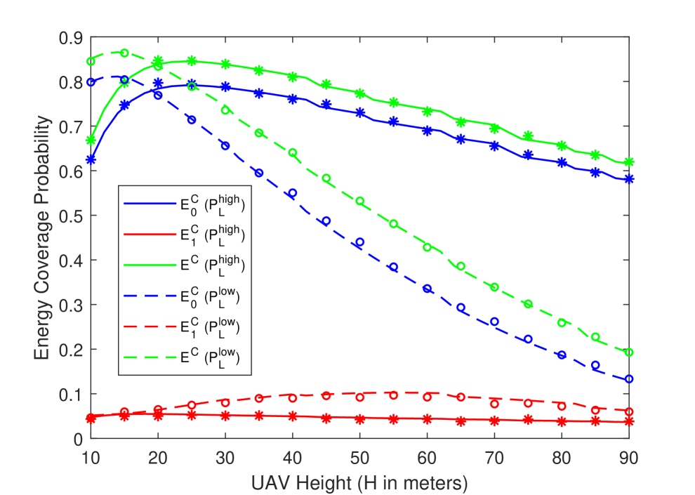
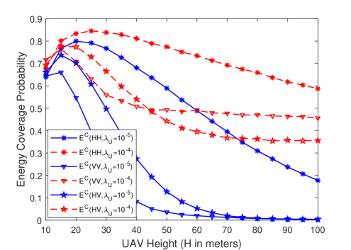
VI-B Impact of UAV Height
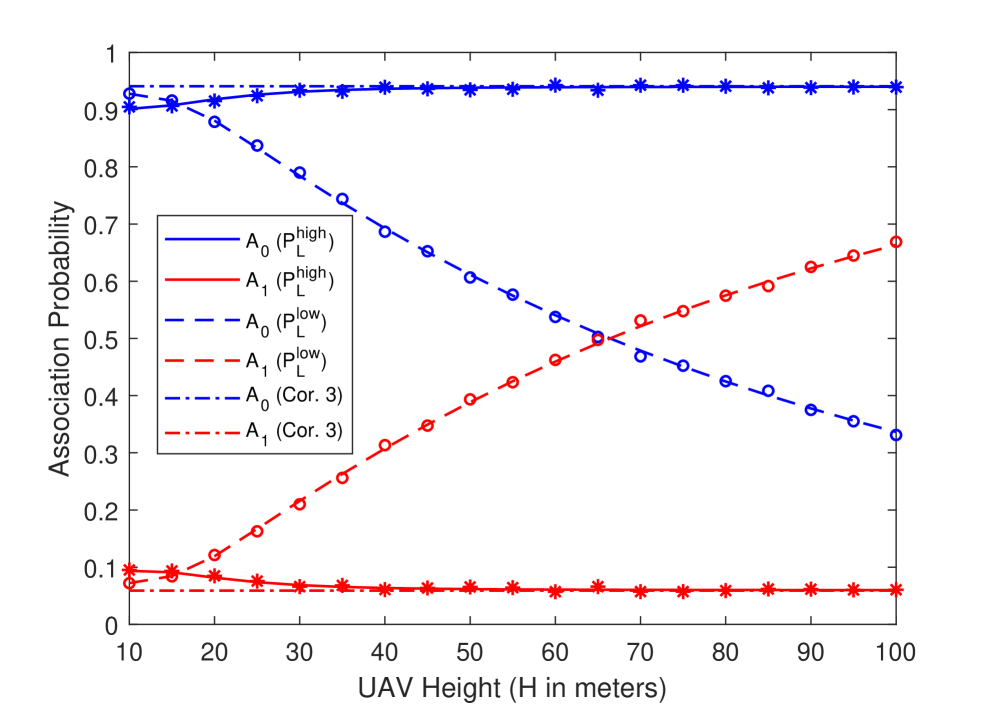
Next, in Figs. 5(a) and 5(b), we plot the association probability and energy coverage probability as a function of UAV height considering the LOS probability functions of both high-altitude and low-altitude models. For the high-altitude model, since LOS probability increases with the increasing UAV height, association probability with the tier UAV increases slightly. On the other hand, LOS probability decreases as a result of the increase in the 3D distance with the increasing UAV height in the low-altitude model. Therefore, more UEs prefer to connect to tier UAVs (i.e., UAVs other than the cluster-center one) at higher values of the UAV height. Also note that the result of the Corollary 3 very closely approximates the association probabilities of the high-altitude model especially as the UAV height increases.
Energy coverage probability of the cluster center UAV, , exhibits similar trends for both types of LOS functions. More specifically, increases first then it starts decreasing with the increasing UAV height. Since the effective antenna gain for HH antenna orientation is an increasing function of UAV height for a fixed cluster size, an initial increase in is expected. However, further increase in UAV height results in a decrease in of both high-altitude and low-altitude models due to the increase in the distance. Therefore, for a fixed cluster size, there exists an optimal UAV height maximizing the network energy coverage, , for both models. On the other hand, optimal height maximizing the in the low-altitude model is lower and decreases faster than that in the high-altitude model because the LOS probability function of the low-altitude model is a decreasing function of distance while the LOS probability function of the high-altitude model is an increasing function of the UAV height (e.g., as seen in Fig. 2). Moreover, since UEs are more compactly distributed around the cluster center UAVs for , energy coverage probability of the tier UAVs, , is relatively small and changes only very slightly for both models.
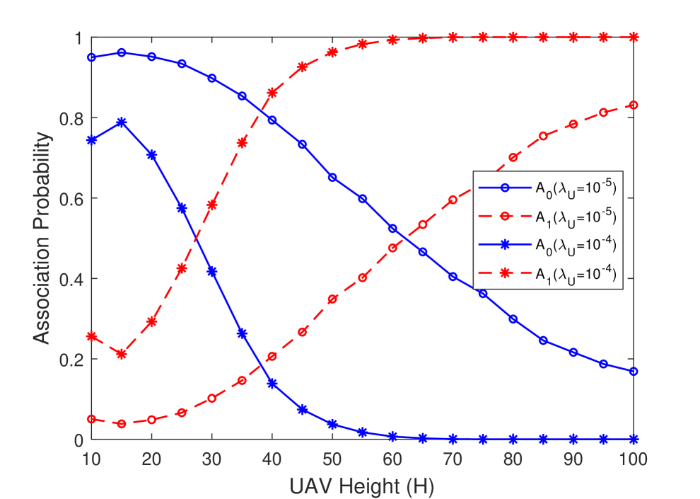
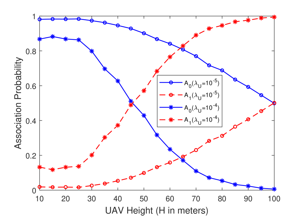
VI-C Impact of Antenna Orientation and UAV Density
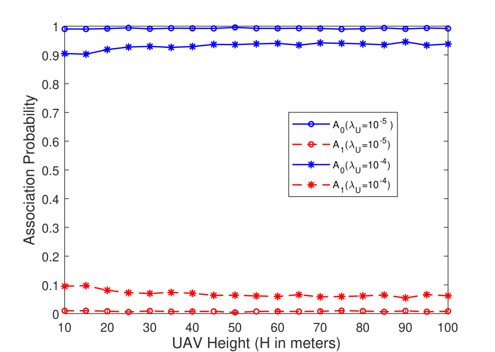
In Figs. 6(a), 6(b) and 6(c), we plot the association probability as a function of UAV height for different values of UAV density for three different antenna orientations considering the high-altitude LOS probability model. Note that since the analysis for VV and HV antenna orientations seems to be intractable, only simulation results are plotted. Since effective antenna gain depends on the sine function of the angle between the UAVs and UEs for HH antenna orientation, UEs prefer to connect to their cluster center UAV, and hence is much larger than even when there is an increase in the number of UAVs (as seen when the UAV density is increased from to ) as shown in Fig. 6(a). Also note that since both antenna gain and LOS probability is an increasing function with UAV height, increase in them can compensate the increasing path loss and the association probabilities remain almost constant.
For the VV antenna orientation, effective antenna gain depends on the cosine of the angle between the UAVs and UEs. For larger values of UAV density, association probability with the tier UAV, , slightly increases with increasing UAV height at first as a result of the increase in both the LOS probability and the effective antenna gain. Subsequently, starts decreasing because the increase in the LOS probability cannot compensate the rapid decrease in the effective antenna gain between the UE and the cluster center UAV. For a less dense network, UEs associate with the cluster-center UAV mostly at lower UAV heights. However, with the increasing height, antenna gain with the cluster-center UAV decreases and consequently, the association probability with tier UAVs, , increases.
Finally, for the HV antenna orientation, effective antenna gain is a function of both cosine and sine of the angle . Association probabilities exhibit similar trends as in the case of VV orientation. However, different from the VV case, since the antenna gain depends on both the cosine and sine functions, association probability with the tier UAV, , is greater than that of the VV orientation.
We also plot the energy coverage probability for different UAV heights, antenna orientations, and UAV densities in Fig. 7. The performance with the HV and VV antenna orientations exhibit similar behaviors as that with the HH antenna orientation which is described in Section VI-B. For both higher-density (i.e., ) and lower-density UAV networks (i.e., ), HH orientation leads the best performance compared to the HV and VV cases. We also note that as the UAV density and UAV height are increased, energy coverage probability with the VV orientation starts exceeding that of the HV case. Therefore, energy coverage performance can be improved by varying the antenna orientations depending on the number of UAVs in the network and their height.
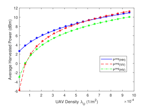
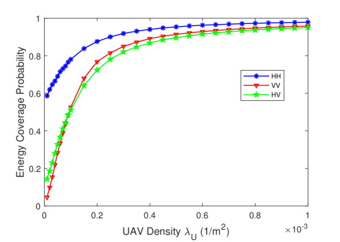
Furthermore, we display the average harvested power and the energy coverage probability as a function of the UAV density for three different antenna orientations considering the high-altitude LOS probability model in Figs. 8 and 9, respectively. Both the average harvested power and the energy coverage probability are increasing functions of the UAV density irrespective of the antenna orientation for a fixed UAV height. Expectedly, adding more UAVs to the network results in an increase in the total power received at the typical UE, and hence the average harvested power grows and the energy coverage performance of the network improves. We also note that HH antenna orientation generally leads to larger average harvested power and energy coverage probability. On the other hand, VV antenna orientation results in a higher average harvested power when the UAV density is sufficiently large due to the fact that one can harvest more power from the dense -tier UAVs with smaller elevation angles when this antenna orientation is used.
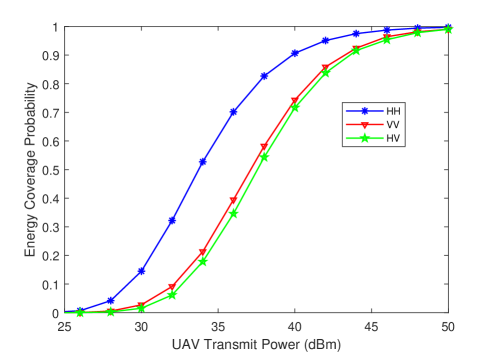
VI-D Impact of UAV Transmit Power
In Fig. 10, we plot the energy coverage probability as a function of the UAV transmit power for three different antenna orientations considering the high-altitude LOS probability model. As expected, energy coverage probability is an increasing function of UAV transmit power. Moreover, HH antenna orientation generally results in a higher energy coverage probability than VV and HV antenna orientations.
VI-E Impact of Energy Outage Threshold
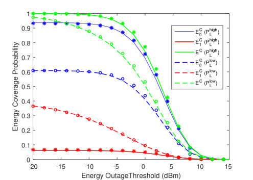
In Fig. 11, we show the energy coverage probabilities of different tiers (i.e., and ) and the total energy coverage probability as a function of the energy outage threshold for both high-altitude and low-altitude models. As seen in Fig. 4(a) and Fig. 5(a), UEs are more likely to be associated with the tier UAV rather than tier UAVs in the high-altitude model when , and hence is much higher than . On the other hand, for the low-altitude model, since association probabilities with each tier are not very different, more UEs can be covered by tier UAVs compared to the high-altitude model. However, is still greater than due to the relatively smaller distance to the cluster-center UAV. We also observe that as a general trend, energy coverage probabilities expectedly diminish with increasing energy outage threshold.
VI-F Impact of Different UAV Heights
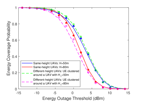
Finally, in Fig. 12, we plot the total energy coverage probabilities as a function of the energy outage threshold using the high-altitude LOS probability function model when UAVs are assumed to be located at different heights. In this setup, we use the same parameters given in Table II with some differences in UAV height and UAV density. More specifically, we consider groups of UAVs located at altitudes m and m with densities and transmit powers dBm. Therefore, transmit power of the UAV is also equal to dBm. Similar to [24], we consider practical values for UAV heights which are around meters.
In Fig. 12, solid lines plot the total energy coverage probabilities when the height is the same for all UAVs. Dashed lines display the coverage probabilities when half of the UAVs are located at height and the other half are located at height , and the typical UE is clustered around a UAV at either height or . As seen in the figure, energy coverage performance of the different-height UAV network is very similar to that of the same-height UAV. For example, if a typical UE is clustered around a UAV at height m, the performance of the different-height UAV network is almost the same with that of the same-height UAV for m. On the other hand, performance of the different-height network when the typical UE is clustered around a UAV at height m is slightly lower than that of the same-height UAV network with m as a result of growing impact of interferences from the UAVs at height m.
VII Conclusion
In this paper, we have analyzed the energy coverage probability of a UAV network with clustered UEs. The UEs are distributed according to a PCP around PPP distributed cluster centers. The UAVs are deployed at a certain height above these cluster centers, which, as a result, represent the projections of UAVs on the ground. UEs are assumed to be associated with the UAV providing the strongest long-term averaged power. In this setting, we have determined the association probabilities and characterized the energy coverage probability. We have analyzed the effect of two different LOS probability functions on the network performance. We have also investigated the impact of practical 3D antenna radiation patterns on the network performance. Furthermore, we have presented energy coverage probability expressions for a more general model in which UAVs are located at different heights.
Via numerical results, we have demonstrated that the standard deviation of UE distribution , UAV height , and antenna orientation have considerable influence on UAV association and energy coverage probabilities. For instance, more widely spread UEs result in a decrease in the total energy coverage probability of the network for both LOS probability models. For a certain cluster size, there exists an optimal UAV height that maximizes the network energy coverage. However, this optimal height depends on the type of the LOS probability model. In particular, low-altitude model features a lower optimal height than the high-altitude model. Although the maximum value of the energy coverage reached at the optimal height is almost the same for both models, low-altitude model has better energy coverage performance at lower heights. On the other hand, high-altitude model performs better at higher heights. These observations indicate that energy coverage performance is greatly affected by the environment. We have also shown that antenna orientation has a significant impact on the energy coverage probability depending on the UAV density. Specifically, better performance can be achieved by changing the antenna orientations according to the number of UAVs in the network and their height. We have also evaluated the average harvested power levels for different antenna orientations at various UAV density levels and computed the energy coverage probability as UAV density, UAV transmission power or energy outage threshold varies and we identified the impact of these different settings on the performance. Finally, we have addressed the performance of the different-height network and noted that UAVs at lower heights can lead to increased interference. Analyzing the performance of a UAV network with simultaneous information and energy transfer remains as future work.
-A Proof of Lemma 1
The CCDF of the path loss from a typical UE to a tier LOS/NLOS UAV is
| (32) | |||
| (33) |
where is given in (1), and is the LOS or NLOS probability depending on whether or . With this, the CCDF of the path loss from a typical UE to a tier UAV given in Lemma 1 can be obtained by summing up over .
-B Proof of Lemma 2
Intensity function for the path loss model from a typical UE to a tier UAV for can be formulated as follows:
| (34) | ||||
| (35) | ||||
| (36) | ||||
| (37) |
where (34) is due to the definition of intensity function for the point process of the path loss. CCDF of the path loss from a typical UE to a tier UAV given in Lemma 2 can be obtained by summing up over .
-C Proof of Lemma 3
Association probability with a tier LOS/NLOS UAV can be expressed as
| (38) | ||||
| (39) | ||||
| (40) |
where (38) uses the fact that LOS and NLOS links in the tier are independent, and (40) incorporates the definition of the CCDF of the path loss. Since the distance between UEs and UAVs is at least , the lower limit of the integration is .
Association probability with a tier LOS/NLOS UAV is given by
| (41) | |||
| (42) |
where , and . (41) makes use of the definition of the association probability and the fact that LOS and NLOS links in the tier are independent, and .
-D Proof of Lemma 4
The total average harvested power at a typical UE can be formulated as
| (43) |
where is the conditional average harvested power given that the UE is associated with a LOS/NLOS UAV in tier , and denotes the association probability. Conditional average harvested power can be obtained as follows:
| (44) | ||||
| (45) |
where (44) follows from the averaging over the fading distribution, inserting the antenna gain for HH antenna orientation and employing Campbell’s theorem, (45) follows from the definitions of and provided in (24) and (25), respectively. Note that the interfering tier UAV and tier UAVs lie outside the exclusion disc with radius and with radius , respectively. Finally, by inserting (15), (16), (45) into (43), the average harvested power expression in (23) can be obtained.
-E Proof of Theorem 1
Given that the UE is associated with a LOS/NLOS UAV in tier , the conditional energy coverage probability is
| (46) | |||
| (47) | |||
| (48) | |||
| (49) |
where , , is the number of terms in the approximation, is the Laplace transform of , and (47) is approximated by following the similar steps in [8]. In (48), we inserted the antenna gain , and the last step in (49) follows from and by noting that Laplace transforms of interference at the UE from different tier UAVs are independent.
Laplace transforms can be determined by employing key characterizations from stochastic geometry. Recall that tier interference arises from the UAV at the cluster center of the typical UE. When the typical UE is associated with a UAV in the tier, Laplace transform of the interference from tier UAV can be formulated as
| (50) | |||
| (51) | |||
| (52) |
where conditioning in (50) is a result of the UAV association policy, i.e., the received power from the interfering tier UAV is less than the received power from the associated UAV, (51) follows from and inserting the antenna gains, in the last step the exclusion disc . Also note that , if the typical UE is associated with tier UAV.
Laplace transform of the interference from tier UAVs is
| (53) | |||
| (54) |
where (53) is obtained by computing the probability generating functional of the PPP, and (54) follows by computing the moment generating function of the exponentially distributed random variable . Note that the interfering tier UAVs lie outside the exclusion disc with radius . Finally, by inserting (15), (16), (28), (29) into (26), energy coverage probability expression in (27) can be obtained.
References
- [1] L. Zhang, H. Zhao, S. Hou, Z. Zhao, H. Xu, X. Wu, Q. Wu, and R. Zhang, “A survey on 5G millimeter wave communications for UAV-assisted wireless networks," IEEE Access, Early Access, Jul. 2019.
- [2] Y. Zeng, Q. Wu, and R. Zhang, “Accessing from the sky: A tutorial on UAV communications for 5G and beyond," Proceedings of the IEEE, vol. 107, no. 12, pp. 2327–2375, Dec. 2019.
- [3] N. H. Motlagh, T. Taleb, and O. Arouk, “Low-altitude unmanned aerial vehicles-based internet of things services: comprehensive survey and future perspectives," IEEE Internet of Things J., vol. 3, no. 6, pp. 899–922, Dec. 2016.
- [4] A. Merwaday, A. Tuncer, A. Kumbhar, and I. Guvenc, “Improved throughput coverage in natural disasters: Unmanned aerial base stations for public-safety communications," IEEE Veh. Techno. Mag., vol. 11, no. 4, pp. 53-60, Dec. 2016.
- [5] R. I. Bor-Yaliniz, and H. Yanikomeroglu, “The new frontier in RAN heterogeneity: Multi-tier drone-cells," IEEE Commun. Mag., vol. 54, no. 11, pp. 48–55, Nov. 2016.
- [6] Y. Zeng, B. Clerckx, and R. Zhang, “Communications and signals design for wireless power transmission," IEEE Trans. Commun., vol. 65, no. 5, pp. 2264–2290, May 2017.
- [7] S. Bi, C. K. Ho, and R. Zhang, “Wireless powered communication: Opportunities and challenges," IEEE Commun. Mag., vol. 53, no. 4, pp. 117–125, Apr. 2015.
- [8] T. A. Khan, A. Alkhateeb, and R. W. Heath, “Millimeter wave energy harvesting," IEEE Trans. Wireless Commun., vol. 15, no. 9, pp. 6048-6062, Sep. 2016.
- [9] A. Sakr and E. Hossain, “Cognitive and energy harvesting-based D2D communication in cellular networks: Stochastic geometry modeling and analysis," IEEE Trans. Commun., vol. 63, pp. 1867-1880, May 2015.
- [10] K. Huang and V. Lau, “Enabling wireless power transfer in cellular networks: Architecture, modeling and deployment," IEEE Trans. Wireless Commun., vol. 13, pp. 902-912, Feb. 2014.
- [11] M. Di Renzo, and W. Lu, “System-level analysis and optimization of cellular networks with simultaneous wireless information and power transfer: Stochastic geometry modeling," IEEE Trans. Veh. Techn., vol. 66, no. 3, pp. 2251-2275, Mar. 2017.
- [12] J. Xu, Y. Zeng, and R. Zhang, “UAV-enabled wireless power transfer: Trajectory design and energy optimization," IEEE Trans. Wireless Commun., vol. 17, no. 8, pp. 5092–5106, Aug. 2018.
- [13] Y. Wu, J. Xu, and L. Qiu, “UAV-enabled wireless power transfer with directional antenna: A two-user case (invited paper)," Intern. Symp. on Wireless Commun. Syst. (ISWCS), pp. 1–6, Aug. 2018.
- [14] Y. Hu, X. Yuan, J. Xu, and A. Schmeink, “Optimal 1D trajectory design for UAV-enabled multiuser wireless power transfer," IEEE Trans. Commun., vol. 67, no. 8, pp. 5674-5688, Aug. 2019.
- [15] L. Xie, J. Xu, and R. Zhang, “Throughput maximization for UAV-enabled wireless powered communication networks," IEEE Internet of Things J., Early Access, Oct. 2018.
- [16] S. Cho, K. Lee, B. Kang, K. Koo, and I. Joe, “Weighted harvest-then-transmit: UAV-enabled wireless powered communication networks," IEEE Access, vol. 6, pp. 72212-72224, Nov. 2018.
- [17] C. Caillouet, T. Razafindralambo, and D. Zorbas, “Optimal placement of drones for fast sensor energy replenishment using wireless power transfer," Wireless Days 2019, Apr. 2019.
- [18] “ When COWs Fly: AT&T Sending LTE Signals from Drones," https://about.att.com/innovationblog/cows_fly, Feb. 2017.
- [19] B. Galkin, J. Kibiłda, and L. A. DaSilva, “Coverage Analysis for Low-Altitude UAV Networks in Urban Environments," Proc. of IEEE Globecom, Dec. 2017.
- [20] V. V. Chetlur, and H. S. Dhillon, “Downlink coverage analysis for a finite 3-D wireless network of unmanned aerial vehicles," IEEE Trans. Commun., vol. 65, no. 10, pp. 4543-4558, Oct. 2017.
- [21] E. Turgut and M. Cenk Gursoy, “Downlink analysis in unmanned aerial vehicle (UAV) assisted cellular networks with clustered users," IEEE Access, vol. 6, pp. 36313-36324, May 2018.
- [22] P. K. Sharma and D. I. Kim, “Coverage probability of 3D mobile UAV networks," IEEE Wireless Commun. Letters, vol. 8, no. 1, pp. 97-100, Feb. 2019.
- [23] L. Zhou, Z. Yang, S. Zhou, and W. Zhang, “Coverage probability analysis of UAV cellular networks in urban environments," IEEE Inter. Conf. on Commun. Workshops (ICC Workshops), pp. 1–6, May 2018.
- [24] C. Liu, M. Ding, C. Ma, Q. Li, Z. Lin, and Y.-C. Liang, “Performance analysis for practical unmanned aerial vehicle networks with LoS/NLoS transmissions," IEEE Inter. Conf. on Commun. Workshops (ICC Workshops), pp. 1–6, May 2018.
- [25] C. Zhang, and W. Zhang, “Spectrum sharing for drone networks," IEEE J. Sel. Areas Commun., vol. 35, no. 1, pp. 136-144, Jan. 2017.
- [26] M. Mozaffari, W. Saad, M. Bennis, and M. Debbah, “Unmanned aerial vehicle with underlaid device-to-device communications: Performance and tradeoffs," IEEE Trans. Wireless Commun., vol. 15, no. 6, Jun. 2016.
- [27] J. Lyu, Y. Zeng, and R. Zhang, “UAV-aided cellular offloading for cellular hotspot," IEEE Trans. Wireless Commun., vol. 17, no. 6, pp. 3988-4001, Jun. 2018.
- [28] R. I. Bor-Yaliniz, A. El-Keyi, and H. Yanikomeroglu, “Efficient 3-D placement of an aerial base station in next generation cellular networks," Proc. of IEEE Int. Conf. Commun. (ICC), pp. 1-5, May 2016.
- [29] M. Mozaffari, W. Saad, M. Bennis, and M. Debbah, “Efficient deployment of multiple unmanned aerial vehicles for optimal wireless coverage," IEEE Wireless Commun. Letters, vol. 20, no. 8, Aug. 2016.
- [30] M. Mozaffari, W. Saad, M. Bennis, and M. Debbah, “Optimal transport theory for power-efficient deployment of unmanned aerial vehicles," Proc. IEEE Int. Conf. Commun. (ICC), May 2016.
- [31] P. Chandhar, D. Danev, and E. G. Larsson, “Massive MIMO for communications with drone swarms," IEEE Trans. Wireless Commun., vol. 17, no. 3, pp. 1604-1629, Mar. 2018.
- [32] G. Geraci, A. Garcia-Rodriguez, L. G. Giordano, D. Lopez-Perez, and E. Bjornson “Understanding UAV Cellular Communications: From Existing Networks to Massive MIMO," IEEE Access, vol. 6, pp. 67853-67865, Nov. 2018.
- [33] J. Lyu and R. Zhang, “Network-connected UAV: 3D system modeling and coverage performance analysis," IEEE Internet of Things J., vol. 6, no. 4, pp. 7048-7060, Aug. 2019.
- [34] W. Khawaja, I. Guvenc, D. Matolak, U.-C. Fiebig, and N. Schneckenberger, “A survey of air-to -ground propagation channel modeling for unmanned aerial vehicles," IEEE Commun. Surveys & Tutorials, vol. 21, no. 3, pp. 2361-2391, May 2019.
- [35] E. Yanmaz, R. Kuschnig, and C. Bettstetter, “Channel measurements over 802.11a-based UAV-to-ground links," Proc. IEEE GLOBECOM Workshops (GC Wkshps), pp. 1280–1284, Dec. 2011.
- [36] E. Yanmaz, R. Kuschnig, and C. Bettstetter, “Achieving air-ground communications in 802.11 networks with three-dimensional aerial mobility," Proc. IEEE INFOCOM, pp. 120–124, Apr. 2013.
- [37] J. Chen, D. Raye, W. Khawaja, P. Sinha, and I. Guvenc, “Impact of 3D UWB antenna radiation pattern on air-to-ground drone connectivity," Proc. of the IEEE Vehicular Techno. Conf. (VTC)-Fall, Aug. 2018.
- [38] A. Kumbhar, I. Guvenc, S. Singh, and A. Tuncer, “Exploiting LTE-advanced HetNets and FeICIC for UAV-assisted public safety communications," IEEE Access, vol. 6, pp. 783-796, Dec. 2018.
- [39] M. Haenggi, Stochastic Geometry for Wireless Networks. Cambridge, U.K.: Cambridge Univ. Press, 2012.
- [40] C. Saha, M. Afshang, and H. S. Dhillon, “Enriched K-Tier HetNet model to enable the analysis of user-centric small cell deployments," IEEE Trans. Wireless Commun., vol. 16, no. 3, Mar. 2017.
- [41] A. Al-Hourani, S. Kandeepan, and S. Lardner, “Optimal LAP altitude for maximum coverage," IEEE Wireless Commun. Letters, vol. 3, no. 6, Dec. 2014.
- [42] 3GPP, “Tr 36.828 (v11.0.0): Further enhancements to lte time division duplex (tdd) for downlink-uplink (dl-ul) interference management and traffic adaptation," 2016.
- [43] X. Wang, E. Turgut, and M. Cenk Gursoy, “Coverage in downlink heterogeneous mmWave cellular networks with user-centric small cell deployment," IEEE Transactions on Vehicular Technology, vol. 68, no. 4, pp. 3513-3533, Apr. 2019.
- [44] E. Turgut, M. Cenk Gursoy, and I. Guvenc, “Energy harvesting in unmanned aerial vehicle networks with 3D antenna radiation patterns," Proc. of the IEEE Vehicular Technology Conference (VTC)-Fall, pp. 1-5, Sep. 2019.