Energy-efficient Hybrid Model Predictive Trajectory Planning for Autonomous Electric Vehicles

Incorporating KERS into trajectory planning has ganined immense traction in research, with two prominent approaches: eco-driving control and energy control strategy. On one hand, examples of eco-driving control approaches include Connected and Autonomous Vehicles (CAVs) which optimizes speed profiles across various scenarios to conserve energy [18]. In addition, Energy Management Systems (EMS) for plug-in hybrid and hybrid vehicles prioritize minimizing powertrain energy consumption while meeting drive power requirements [8]. Automotive eco-driving is currently regarded as an effective method in enhancing vehicle energy-efficiency without extensive hardware integration [18]. On the other hand, energy control strategy primarily focuses on planning the most energy-efficient trajectory and speed for the vehicle by leveraging a dynamic model of the EV [19]. For example, the work [20] introduced an intelligent energy-saving control strategy for EVs, which implements the motion of the preceding vehicle to distinguish between four distinct scenarios and inform control decisions. The work cited in [21] introduces an integrated energy recovery strategy for regenerative braking systems in intelligent, four-wheel independent drive electric vehicles. This approach spans planning to control, addressing energy recovery across three distinct layers. It advocates for trajectory optimization in electric vehicles using an inverse dynamics model and servo constraints, aiming to enhance vehicle energy efficiency through strategic trajectory planning.

Additionally, the work cited in [22] presented an energy control strategy for self-driving electric vehicles navigating intersections with continuous speed limit signals. This strategy enhances vehicle energy efficiency under continuous traffic light conditions by regulating vehicle speed.

To our best knowledge, most trajectory planning primarily focuses on the physical conditions and driving strategy of the car, with few works incorporating KERS into planner.

Given the central emphasis on energy-efficiency within this paper, the influence of car steering effects is deliberately excluded from consideration in this study.

To achieve simulation control, here we construct an automobile kinematic model that adheres to the following constraints under free motion: (1) Input parameters of the kinematic model encompass road slope, air resistance coefficient, ground friction coefficient, and car windward area. (2) Optimal road surface adhesion coefficients ensure balanced adhesion on both sides, mitigating any potential side-slip phenomena. (3) Motion heading angle constrains the car’s trajectory. (4) The vehicle is treated as a rigid body rather than a mere mass. The vehicle kinematics model is depicted in Figure 1.

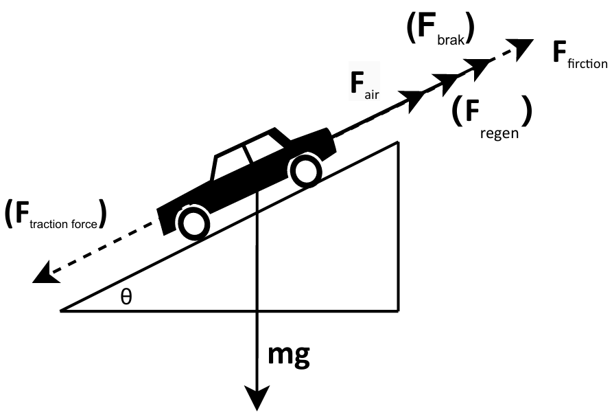
The air resistance acting on the vehicle is:

$$F_{\text{air}}=\frac{1}{2}\rho v^{2}c_{d}A$$

(1)

where $\rho$ denotes the air density, $v$ denotes the speed of the car, $C_{d}$ is the coefficient of air resistance, and $A$ is the windward area of the car.

$$F_{\text{friction}}=\mu mg\cos(\theta)$$

(2)

The forces induced by slope are:

$$F_{\text{slope}}=mg\sin(\theta)$$

(3)

Let $P_{\text{ENG}}$ and $P_{\text{REGEN}}$ denote the engine output and maximum power of the energy recovery system, respectively. Thus, the maximum forces from KERS and the motor are $F_{\text{REGEN}}$ and $F_{\text{ENG}}$. Since $F_{\text{REGEN}}$ represents resistance and $F_{\text{ENG}}$ denotes power, these systems are mutually exclusive, meaning the energy recovery system is inactive during vehicle acceleration.

Consequently, the kinematic relationship during vehicle acceleration can be expressed as follows:

$$ma_{ac}=F_{\text{traction force}}-\frac{1}{2}\rho v^{2}c_{d}A-\mu mg\cos(\theta)\pm mg\sin(\theta)$$

(4)

The dynamics relationships during deceleration are:

$$ma_{Dec}=-\biggl{(}\frac{1}{2}\rho v^{2}C_{d}A+\mu mg\cos(\theta)\\ +F_{\text{REGEN}}+F_{\text{brake}}\biggr{)}+mg\sin(\theta)$$

(5)

Our focus lies in planning of the car’s driving and formulating the corresponding cost functions for optimal planning. During the acceleration phase, particular emphasis is placed on achieving energy-saving travel speed and energy-saving acceleration.

It has been shown that maintaining a steady driving behavior results in the lowest energy consumption[26]. This ”steady driving behavior” is achieved via accelerating at a low rate to achieve a constant speed, thereby minimizing energy consumption. Furthermore, it has been observed that the relationship between the vehicle’s driving speed and energy consumption can be approximated by a quadratic equation.

Therefore, during uniform cruise (where acceleration is zero), the vehicle must adhere to the optimal cruise speed, denoted as $V_{\text{OPT}}$. This optimal cruise speed, $V_{\text{OPT}}$, is determined by the vehicle’s optimal engine power and external environmental dynamics wich can be expressed as:

$$V_{\text{OPT}}=\frac{F_{\text{Air}}+F_{\text{Friction}}+F_{\text{Slope}}}{P_{\text{Opt}}}$$

(6)

where $P_{\text{opt}}$ represents a constant value determined by the electric vehicle’s motor.

During acceleration, the EVs should enter the constant speed phase with optimal acceleration without violating constraints.

The constraints for the dynamics model are outlined as follows:

1. 1.

   The acceleration of the car must adhere to the limitation of the maximum power output of the motor.

2. 2.

   Objective constraints govern the braking process of the vehicle.

3. 3.

   The vehicle operation is mandated by formal road regulations.

According to the studies [26][27][26][28], there is an optimal acceleration with least energy consumption. In this process, the optimal acceleration of the vehicle is modeled via dynamic equation as follows:

$$a_{\text{Acc\_Opt}}=\frac{\frac{P_{2}}{v}-\left(f_{\text{Air}}+f_{\text{Friction}}+f_{\text{Slope}}\right)}{m}$$

(7)

where $P_{\text{2}}$ refers to the optimal output power of the motor or engine in the acceleration phase, which could make acceleration achieve the most energy-efficient.Thus, we identify the acceleration in this state of acceleration as the optimal acceleration.

During deceleration, the EVs decelerates at the optimal deceleration speed fllowing the same constraints. According to [8][29], when the vehicle’s kinetic energy recovery system decelerates at a specific speed range, it has the highest kinetic energy recovery efficiency. It is deduced that there is an optimal deceleration in the process of vehicle deceleration, to maximize the efficiency of the kinetic energy recovery system. When this optimal braking condition is met, the vehicle should not apply additional braking force at the brake end. In this process, the optimal vehicle deceleration by dynamic relationship recurrence is as follows:

$$a_{\text{Opt\_Dec}}=\frac{\frac{P_{m}}{v}+f_{\text{Air}}+f_{\text{Friction}}+f_{\text{Slope}}}{m}$$

(8)

Where $P_{\text{m}}$ is the power of the vehicle kinetic energy system with maximum energy-efficiency, which is determined by the configuration of the vehicle kinetic energy recovery system which could make deceleration achieve the most energy-efficient. So we identify the deceleration in this accelerated state as the optimal deceleration.

Our proposed strategy aims to achieve optimal energy efficiency across acceleration, deceleration, and uniform cruising phases. This strategy is designed to optimize the speed and route planning of the autonomous driving system, ensuring alignment with the vehicle’s optimal acceleration and deceleration requirements.

We implement a uniform random sampling within a discrete space and subsequently link the sampling points using a quintic polynomial (illustrated in Figure 3). Upon establishing suitable boundary conditions, the trajectory is formulated through the connection of these points with a quintic polynomial.

The quintic polynomial is expressed as follows:

$$l=f(s)=a_{0}+a_{1}s+a_{2}s^{2}+a_{3}s^{3}+a_{4}s^{4}+a_{5}s^{5}$$

(9)

Given a function $g(s,l)$, the derivatives of the function with respect to the variables $s$ and $l$ are denoted as follows:

• •

  $g^{\prime}(s,l)$ denotes the first derivative of $g$ with respect to both $s$ and $l$.

• •

  Higher derivatives follow similarly, e.g., $g^{\prime\prime}(s,l)$ for the second derivative.

The basic cost function is defined as follows:

$$C_{\text{Obs}}(d)=\begin{cases}0&\text{x}>d_{1}\\ 2d+b&\text{d}_{2}<d<d_{1}\\ +\infty&\text{x}<d_{2}\end{cases}$$

(10)

Where, $h(d)$ is defined as a segmented function. In the current coordinate system, the variable $d$ represents the distance between the vehicle and the obstacle. Let the safety interval at the current speed be denoted by the interval $[d_{1},d_{2}]$.

	$\displaystyle C_{\text{Sm}}(f)$	$\displaystyle=w_{1}\int(f^{\prime}(s))^{2}\,ds+w_{2}\int(f^{\prime\prime}(s))^{2}\,ds$
		$\displaystyle\quad+w_{3}\int(f^{\prime\prime\prime}(s))^{2}\,ds.$		(11)

$$C_{\text{Re}}(f)=\int g(s)^{2}\,ds$$

(12)

Equation (11) defines the cost function for the smoothness of the planned trajectory, where $f^{\prime}(s_{i})^{2}$ expresses how similar it is to a straight line. The terms $f^{\prime\prime}(s)^{2}\,ds$ and $f^{\prime\prime\prime}(s)^{2}\,ds$ quantify the trajectory’s curvature and the rate of change of curvature, respectively. Equation (10) details the distance between the vehicle and an obstacle, while Equation (12) describes the distance between the vehicle and the reference line. Additionally, $C_{\text{sm}}$ denotes the cost associated with trajectory smoothing. The function $C_{\text{Obs}}$ calculates the cost related to the distance from obstacles. Define the reference line function as $g$$(s)$ and the function $g(s)\,ds$  indicates the cost from the reference line.

In Equation (10), the selection of parameters $d_{1}$ and $d_{2}$ critically influences the choice of drag acceleration during the vehicle’s deceleration phase and directly impacts the vehicle’s energy consumption. The procedure for calculating the optimal values of $d_{1}$ and $d_{2}$ for the vehicle is outlined below:

$$F_{\text{Stop\_Max}}=F_{\text{Regen}}+F_{\text{Res}}+F_{\text{Slope}}+F_{\text{Friction}}+F_{\text{Air}}$$

(13)

Thus,

$$a_{\text{Dec\_Max}}=\frac{F_{\text{Stop\_Max}}}{m}$$

(14)

$$d_{2}=\frac{v_{f}^{2}-v_{\text{Cur}}^{2}}{2a_{\text{Dec\_Max}}}$$

(15)

The total cost function of trajectory dynamic programming process is as follows:

$$C_{\text{Total}}=W_{\text{Obs}}C_{\text{Obs}}+W_{\text{Sm}}C_{\text{Sm}}+W_{\text{Re}}C_{\text{Re}}$$

(16)

In adherence to the energy conservation strategic imperatives of EHMPP, the weighting factor $W_{\text{Sm}}$ is considerably greater than $W_{\text{Re}}$. This preference is to ensure the vehicle’s trajectory approximates a straight line as closely as possible, thereby mitigating the kinetic energy loss associated with recurrent adjustments of the method disk. After defining the cost function, we use dynamic programming to obtain rough solutions that provide convex space for QP.

The quadratic programming will search in the convex space opened up by the DP, as shown in Figure 4. QP mainly uses the cost function to find the optimal solution in this convex space, that is, the trajectory is output to the control module.

In the adopted coordinate framework, the coordinates corresponding to the path point are denoted by $(s_{i},t_{i})$, while the subsequent point’s coordinates are represented by $(s_{i+1},t_{i+1})$. QP is utilized to optimize the first and second derivatives of specified points along the trajectory. The trajectory is formulated as a quintic polynomial curve $l$ = $f(s)$, with the third derivative maintained as a constant, ensuring that all derivatives of $f(s)$ of order four and higher are zero between any two consecutive points $i$ and $i+1$. Subject to the continuity constraints on the second derivative of $f(s)$ and vehicular collision avoidance, the trajectory optimization cost, following a finite-term Taylor expansion at points $i$ and $i+1$. Upon incorporating the cost near the reference line, as formulated through quadratic programming, is delineated as follows:

	$\displaystyle C_{\text{total}}(f)=$	$\displaystyle\,w_{1}\int(f^{\prime}(s))^{2}\,ds+w_{2}\int(f^{\prime\prime}(s))^{2}\,ds$
		$\displaystyle+w_{3}\int(f^{\prime\prime\prime}(s))^{2}\,ds+w_{4}\int(f(s)-g(s))^{2}\,ds.$		(17)

Where, $g(s)$ refers to the rough solution trajectory of DP. The cost function $(f(s)-g(s))^{2}$ quantifies the cost to the reference line. A greater path deviation results in an increased cost function value, thereby imposing a higher deviation penalty. The $(f^{\prime}(s))^{2}$ represents the cost function for trajectory smoothness. The $(f^{\prime\prime}(s))^{2}$ is the curvature cost and $(f^{\prime\prime\prime}(s))^{2}$ is the curvature continuity cost.

After completing trajectory planning, we need to carry out velocity planning on this basis.

Similar to trajectory planning, velocity planning requires a combination of dynamic and quadratic programming for similar reasons. A new Frenet coordinate system is established with the trajectory as the coordinate axis. In order to simplify the calculation, we regard the obstacle as a particle and construct the ST diagram as follows:

In EHMPP, the acceleration stage cost function comprises three components: obstacle, optimal acceleration, and recommended speed costs. In the space-time (ST) diagram, the generated trajectory is represented by $S$$(t)$ .Simplified within the ST diagram, the obstacle cost represents the minimal distance from a point to a line segment.To differentiate from the previous stage, we denote the derivative of the function $f(s)$, representing acceleration, by $\dot{s}_{i}$ and so forth. Accordingly, the obstacle cost function is derived as follows:

$$C_{\text{obs}}=\begin{cases}0&\text{if }|d_{\text{min}}|>d_{1}\\ \frac{A}{d_{\text{min}}-d_{2}}&\text{if }d_{2}<|d_{\text{min}}|<d_{1}\\ +\infty&\text{if }|d_{\text{min}}|<d_{2}\end{cases}$$

(18)

Where, $d_{\text{min}}$ refers to the minimum distance from the obstacle.

For simplicity, the derivatives are approx-imated by the finite difference method. Simultaneously, we discretize the trajectories into discrete points and evaluate the associated cost function. The cost function for reference speed of the point is defined as:

$$C_{\text{ref\_speed}}=W_{\text{ref\_speed}}(\dot{s}_{i}-v_{\text{opt}})^{2}$$

where $\dot{s}_{i}$ represents the actual speed of the vehicle, and $v_{\text{opt}}$ is the optimal speed.

EHMPP aims to maintain as Optimal acceleration as possible and accelerate gently to achieve optimal acceleration energy consumption:

$$C_{\text{acc}}=W_{\text{acc}}(\ddot{s}_{i}-a_{\text{acc\_opt}})^{2}+W_{\text{je}}(\dddot{s}_{i})^{2}$$

where $\ddot{s}_{i}$ is the actual acceleration, and $\dddot{s}_{i}$ is the jerk of the vehicle. Therefore, we define the cost function of speed planning in the acceleration phase as follows:

$$C_{\text{acc\_total}}=W_{1}C_{\text{ref\_speed}}+W_{2}C_{\text{acc}}+W_{3}C_{\text{obs}}$$

(19)

In the deceleration phase, EHMPP considers not only the minimum braking distance within the path planning phase but also the optimal drag acceleration during deceleration. This approach ensures the kinetic energy recovery system operates at maximal power. The cost function for acceleration in the deceleration phase is defined accordingly:

$$C_{\text{dec}}=W_{\text{acc}}(\ddot{s}_{i}-a_{\text{dec\_opt}})^{2}+W_{\text{je}}(\dddot{s}_{i})^{2}$$

At the same time, obstacle cost and optimal speed cost need to be considered. The overall cost function is constructed as follows:

$$C_{\text{dec\_total}}=W_{1}C_{\text{ref\_speed}}+W_{2}C_{\text{dec}}+W_{3}C_{\text{obs}}$$

(20)

During constant cruising, EHMPP solely considers the recommended speed cost:

$$C_{\text{con\_total}}=W_{1}C_{\text{ref\_speed}}+W_{3}C_{\text{obs}}$$

(21)

Upon calculating the cost for all points, the endpoint for velocity planning is determined by traversing the upper and right boundaries to identify the point with minimal cost. Subsequently, the preliminary solution for the dynamic programming model is derived through a reverse solution process.

After deriving an initial solution, the QP algorithm extends its search within the opened convex space. At this juncture, QP primarily functions to refine the solution, ensuring smoothness and adherence to predefined constraints. The cost function employed by QP at each stage is detailed below:

Acceleration Phase Cost:

$$C_{\text{QP\_acc}}=\sum(W_{1}C_{\text{ref\_speed}}+W_{2}C_{\text{acc}}+W_{3}C_{\text{obs}})$$

(22)

Deceleration Phase Cost:

$$C_{\text{QP\_dec}}=\sum(W_{1}C_{\text{ref\_speed}}+W_{2}C_{\text{dec}}+W_{3}C_{\text{obs}})$$

(23)

Constant Cruising Phase Cost:

$$C_{\text{QP\_cru}}=\sum(W_{1}C_{\text{ref\_speed}}+W_{3}C_{\text{obs}})$$

(24)

The subsequent processing of the generated trajectory and velocity plans falls outside the scope of this discourse and, as such, will not be elaborated upon.

References

- [1] V. Nimesh, R. Kumari, N. Soni, A. K. Goswami, and V. M. Reddy, “Implication viability assessment of electric vehicles for different regions: An approach of life cycle assessment considering exergy analysis and battery degradation,” Energy Conversion and Management, vol. 237, p. 114104, 2021.
- [2] A. K. Venkitaraman and V. S. R. Kosuru, “A review on autonomous electric vehicle communication networks-progress, methods and challenges,” World Journal of Advanced Research and Reviews, vol. 16, no. 3, pp. 013–024, 2022.
- [3] I. Miri, A. Fotouhi, and N. Ewin, “Electric vehicle energy consumption modelling and estimation—a case study,” International Journal of Energy Research, vol. 45, no. 1, pp. 501–520, 2021.
- [4] H. Qin, S. Shao, T. Wang, X. Yu, Y. Jiang, and Z. Cao, “Review of autonomous path planning algorithms for mobile robots,” Drones, vol. 7, no. 3, p. 211, 2023.
- [5] A.-E. Taha and N. AbuAli, “Route planning considerations for autonomous vehicles,” IEEE Communications Magazine, vol. 56, no. 10, pp. 78–84, 2018.
- [6] H. Fan, F. Zhu, C. Liu, L. Zhang, L. Zhuang, D. Li, W. Zhu, J. Hu, H. Li, and Q. Kong, “Baidu apollo em motion planner,” arXiv preprint arXiv:1807.08048, 2018.
- [7] Y. Na, Y. Li, D. Chen, Y. Yao, T. Li, H. Liu, and K. Wang, “Optimal energy consumption path planning for unmanned aerial vehicles based on improved particle swarm optimization,” Sustainability, vol. 15, no. 16, p. 12101, 2023.
- [8] C. Armenta-Déu and H. Cortés, “Analysis of kinetic energy recovery systems in electric vehicles,” Vehicles, vol. 5, no. 2, pp. 387–403, 2023.
- [9] Z. Lv and W. Shang, “Impacts of intelligent transportation systems on energy conservation and emission reduction of transport systems: A comprehensive review,” Green Technologies and Sustainability, vol. 1, no. 1, p. 100002, 2023.
- [10] Q. He, Y. Yang, C. Luo, J. Zhai, R. Luo, and C. Fu, “Energy recovery strategy optimization of dual-motor drive electric vehicle based on braking safety and efficient recovery,” Energy, vol. 248, p. 123543, 2022.
- [11] V. Rakov, A. Kapustin, and I. Danilov, “Study of braking energy recovery impact on cost-efficiency and environmental safety of vehicle,” Transportation Research Procedia, vol. 50, pp. 559–565, 2020.
- [12] J. Ko, S. Ko, I.-S. Kim, D. Hyun, and H. Kim, “Co-operative control for regenerative braking and friction braking to increase energy recovery without wheel lock,” International journal of automotive technology, vol. 15, pp. 253–262, 2014.
- [13] J. Ko, S. Ko, H. Son, B. Yoo, J. Cheon, and H. Kim, “Development of brake system and regenerative braking cooperative control algorithm for automatic-transmission-based hybrid electric vehicles,” IEEE Transactions on Vehicular Technology, vol. 64, no. 2, pp. 431–440, 2014.
- [14] H. Pan, L. Qi, Z. Zhang, and J. Yan, “Kinetic energy harvesting technologies for applications in land transportation: A comprehensive review,” Applied Energy, vol. 286, p. 116518, 2021.
- [15] W. Zhang, X. Fang, and C. Sun, “The alternative path for fossil oil: Electric vehicles or hydrogen fuel cell vehicles?,” Journal of Environmental Management, vol. 341, p. 118019, 2023.
- [16] M. Reda, A. Onsy, A. Y. Haikal, and A. Ghanbari, “Path planning algorithms in the autonomous driving system: A comprehensive review,” Robotics and Autonomous Systems, vol. 174, p. 104630, 2024.
- [17] W. Yu and R. Wang, “Development and performance evaluation of a comprehensive automotive energy recovery system with a refined energy management strategy,” Energy, vol. 189, p. 116365, 2019.
- [18] C. Yang, M. Zha, W. Wang, K. Liu, and C. Xiang, “Efficient energy management strategy for hybrid electric vehicles/plug-in hybrid electric vehicles: review and recent advances under intelligent transportation system,” IET Intelligent Transport Systems, vol. 14, no. 7, pp. 702–711, 2020.
- [19] C. Min, Y. Pan, W. Dai, I. Kawsar, Z. Li, and G. Wang, “Trajectory optimization of an electric vehicle with minimum energy consumption using inverse dynamics model and servo constraints,” Mechanism and Machine Theory, vol. 181, p. 105185, 2023.
- [20] L. Xie, Y. Luo, D. Zhang, R. Chen, and K. Li, “Intelligent energy-saving control strategy for electric vehicle based on preceding vehicle movement,” Mechanical Systems and Signal Processing, vol. 130, pp. 484–501, 2019.
- [21] L. Li, X. Ping, J. Shi, X. Wang, and X. Wu, “Energy recovery strategy for regenerative braking system of intelligent four-wheel independent drive electric vehicles,” IET Intelligent Transport Systems, vol. 15, no. 1, pp. 119–131, 2021.
- [22] J. Liu, C. Wang, and W. Zhao, “An eco-driving strategy for autonomous electric vehicles crossing continuous speed-limit signalized intersections,” Energy, p. 130829, 2024.
- [23] R. Bellman, “Dynamic programming,” science, vol. 153, no. 3731, pp. 34–37, 1966.
- [24] B. Li, Q. Kong, Y. Zhang, Z. Shao, Y. Wang, X. Peng, and D. Yan, “On-road trajectory planning with spatio-temporal rrt* and always-feasible quadratic program,” in 2020 IEEE 16th International Conference on Automation Science and Engineering (CASE), pp. 942–947, IEEE, 2020.
- [25] Y. Liu, F. Zha, M. Li, W. Guo, Y. Jia, P. Wang, Y. Zang, and L. Sun, “Creating better collision-free trajectory for robot motion planning by linearly constrained quadratic programming,” frontiers in Neurorobotics, vol. 15, p. 724116, 2021.
- [26] R. Galvin, “Energy consumption effects of speed and acceleration in electric vehicles: Laboratory case studies and implications for drivers and policymakers,” Transportation Research Part D: Transport and Environment, vol. 53, pp. 234–248, 2017.
- [27] X. Wu, D. Freese, A. Cabrera, and W. A. Kitch, “Electric vehicles’ energy consumption measurement and estimation,” Transportation Research Part D: Transport and Environment, vol. 34, pp. 52–67, 2015.
- [28] J. Zhang, Z. Wang, P. Liu, and Z. Zhang, “Energy consumption analysis and prediction of electric vehicles based on real-world driving data,” Applied Energy, vol. 275, p. 115408, 2020.
- [29] B. Demirkale and F. Güven, “Investigation of kinetic energy recovery systems usage in electric vehicles,” Sakarya University Journal of Science, vol. 21, no. 6, pp. 1550–1557, 2017.