Energy-Efficient Designs for SIM-Based Broadcast MIMO Systems

Nemanja Stefan Perović, Eduard E. Bahingayi, and Le-Nam Tran N. S. Perović was with Université Paris-Saclay, CNRS, CentraleSupélec, Laboratoire des Signaux et Systèmes, 3 Rue Joliot-Curie, 91192 Gif-sur-Yvette, France (Email: [email protected]).Eduard E. Bahingayi and Le-Nam Tran are with the School of Electrical and Electronic Engineering, University College Dublin, Belfield, Dublin 4, D04 V1W8, Ireland (Email: [email protected], [email protected]).

Abstract

Stacked intelligent metasurface (SIM), which consists of multiple layers of intelligent metasurfaces, is emerging as a promising solution for future wireless communication systems. In this timely context, we focus on broadcast multiple-input multiple-output (MIMO) systems and aim to characterize their energy efficiency (EE) performance. To gain a comprehensive understanding of the potential of SIM, we consider both dirty paper coding (DPC) and linear precoding and formulate the corresponding EE maximization problems. For DPC, we employ the broadcast channel (BC)- multiple-access channel (MAC) duality to obtain an equivalent problem, and optimize users’ covariance matrices using the successive convex approximation (SCA) method, which is based on a tight lower bound of the achievable sum-rate, in combination with Dinkelbach’s method. Since optimizing the phase shifts of the SIM meta-elements is an optimization problem of extremely large size, we adopt a conventional projected gradient-based method for its simplicity. A similar approach is derived for the case of linear precoding. Simulation results show that the proposed optimization methods for the considered SIM-based systems can significantly improve the EE, compared to the conventional counterparts. Also, we demonstrate that the number of SIM meta-elements and their distribution across the SIM layers have a significant impact on both the achievable sum-rate and EE performance.

Index Terms:

Optimization, broadcast, EE, MIMO, stacked intelligent metasurface (SIM), multi-user.

I Introduction

The framework for the future development of International Mobile Telecommunications (IMT) for 2030 highlights sustainability as a fundamental goal for future communication systems [1]. This means that these systems are expected to be designed with minimal environmental impact, focusing on the efficient use of resources, reducing power consumption, and lowering greenhouse gas emissions. Due to this, the study and development of energy-efficient wireless communications have recently attracted much of attention. At the same time, the global mobile network data traffic is expected to reach 563 exabytes (EBs) by 2029 [2]. To accommodate such a high volume of data traffic, existing network technologies need to evolve, providing additional capabilities. For example, conventional MIMO systems are advancing toward massive MIMO (mMIMO) and ultra-massive MIMO (umMIMO) systems. However, a large number of radio frequency (RF) chains required to support mMIMO transmissions results in substantial power consumption, which leads to an unsustainable and energy inefficient communication model.

A promising technical solution that addresses the growing demand for higher data rates while simultaneously enhancing EE is based on the use of intelligent metasurfaces, specifically reconfigurable intelligent surfaces. RISs are composed of a large number of programmable metamaterial or tiny discrete antenna elements. Each of these elements is capable, using integrated electronic circuits, of dynamically adjusting its electromagnetic (EM) properties (i.e., to form EM fields with controllable amplitudes, phases, polarization) and consequently its EM response to the incoming waves. In this way, RISs can modify the incoming waves in a programmable and controllable manner [3]. This capability allows RISs to simultaneously improve multiple performance metrics, such as spectrum efficiency, EE, coverage. Unfortunately, the multiplicative effect of the path loss of the RIS-assisted links significantly limits the potential EE gains from RIS deployment.

To address the critical issue of RIS, several innovative approaches have been proposed that utilize metamaterial-based antenna technologies instead of conventional antenna arrays in mMIMO transceiver design. These include holographic radio, dynamic metasurface antennas and SIMs. Holographic radio, also known as holographic MIMO (HMIMO), is a hybrid transceiver architecture that achieves high directive gain, spectral efficiency and EE by incorporating a continuous structure of densely packing sub-wavelength metamaterial antenna elements. These element, combined with holographic techniques, are capable of recording and reconstructing the amplitude and the phase of wave fronts [4]. The significantly lower power consumption of HMIMO allows for the deployment of a greater number of antenna elements compared to traditional mMIMO, resulting in higher EE [5]. Similarly, DMAs consist of multiple microstrips, each composed of a multitude of metamaterial radiating elements and connected to a single RF chain [6]. Due to this, DMAs achieve better EE performance than even hybrid analog-to-digital (A/D) architectures, since they do not need additional power to support numerous phase shifters [7]. However, both HMIMOs and DMAs are single layer matasuface structures, which may require a very large number of elements due to practical hardware constraints that limit the number of tunable amplitudes/phases associated with each meta-element.

In contrast, SIMs represent the latest advancement in metamaterial-based antenna technologies. SIMs consist of multiple parallel metasurface layers, each accommodating numerous meta-elements with programmable phase characteristics. These layers are integrated with conventional radio transceivers that employ a small to moderate number of active antennas. The concept of SIMs draws inspiration from the architecture of a deep neural network (DNN), which is a multi-layer neuron structure capable of implementing various functions [8]. Similarly, SIMs can efficiently implement different signal processing tasks, such as transmit precoding and receive combining, directly in the EM domain when properly controlled and programmed. Hence, SIMs have the potential to substantially improve the performance metrics of conventional communication systems, such as the achievable rate and the EE, while requiring minimal additional hardware complexity.

In [9], SIMs were exploited to implement a 2D discrete Fourier transform (DFT) for direction of arrival direction of arrival (DOA) estimation. Moreover, a hybrid channel estimator was proposed in [10], in which the received training symbols were initially processed in the wave domain and subsequently in the digital domain. In [11], the authors jointly optimized the transmit beamforming at the base station (BS) and the SIM phase shifts, to minimize the Cramer-Rao bound (CRB) for target estimation. Using an experimental SIM platform, they evaluated the performance of the proposed algorithms for communication and sensing tasks.

A general path loss model for an SIM-assisted wireless communication system was developed in [12], based on which, an algorithm aimed at maximizing the received power was derived. In [13], the authors studied the achievable sum-rate maximization problem for a downlink channel between a SIM-assisted BS and multiple single-antenna users. The achievable rate optimization for a downlink multi-user SIM-assisted system using statistical channel state information (CSI) was proposed in [14]. Utilizing statistical CSI, the ergodic sum-rate was optimized for a satellite communication system in [15]. In [16], a joint optimization of the SIM phase shifts and transmit power allocation for maximizing the sum-rate in a SIM-assisted multi-user multiple-input single-output (MISO) communication system was implemented, employing a deep reinforcement learning (DRL) approach. In [17], the authors optimized the achievable rate in an uplink SIM-based cell-free MIMO architecture with distributed signal processing. In this setup, each access point (AP) performs local detection of user information, and a central processing unit (CPU) subsequently combines these local estimates to recover the final user information.

The integration of SIMs with transmitters and receivers into a so-called SIM-based HMIMO system, which performs signal precoding and combining in the wave domain, was proposed in [18]. The introduced channel fitting approach enables the SIM-based HMIMO system to achieve significant channel capacity gains compared to mMIMO and RIS-assisted counterparts. Furthermore, the optimization of achievable rates for the SIM-based HMIMO system was studied in [19]. An approach for the mutual information maximization in a SIM-based HMIMO system with discrete signaling was presented in [20], using the cutoff rate as an alternative metric. This study demonstrates that incorporating even a small-scale digital precoder into the system can substantially increase the mutual information performance.

Despite the extensive research summarized in the aforementioned papers, the EE analysis of SIM-assisted MIMO systems remains unexplored. Motivated by this gap, we aim to maximize the EE for a SIM-aided broadcast system with DPC and linear precoding. To find the maximum achievable EE in the case of DPC, we formulate a joint optimization problem of the covariance matrix of the transmitted signal and the phase shifts of the SIM meta-elements. For linear precoding, which is more practical, we consider a joint optimization problem of the transmit signal precoding and the phase shifts of the SIM meta-elements. In both cases, the BS has a limited total power budget and the SIM meta-elements are subject to the unit modulus constraint. The main contributions of this paper are summarized as follows:

•

For DPC, we exploit the well-known Gaussian MIMO BC-MAC duality, reformulating the original EEmax problem as a function of the users’ covariance matrices in the MAC and the phase shifts of the SIM meta-elements. In the context of the adopted AO framework, we present an efficient solution for optimizing the users’ covariance matrices. This solution is based on a tight and concave lower bound of the achievable sum-rate, which is derived using the SCA method. By applying Dinkelbach’s method, we then obtain the optimal users’ covariance matrices by closed-form expressions. Our complexity analysis demonstrates that our proposed method has significantly lower complexity compared to an existing solution. For the optimization of the phase shifts of the SIM meta-elements, we employ a conventional projected gradient-based method, updating all SIM layers in parallel. This approach is viable considering the large size of this problem. In this context, we derive closed-form expressions for the complex-valued gradients involved.
•

For linear precoding, we leverage an interesting recent result for the sum-rate maximization that allows for reformulating the considered EEmax problem as an equivalent one, but with a greatly reduced dimension. After this important step, we again invoke the SCA method to derive a quadratic lower bound of the achievable sum-rate and approximate the EEmax problem as a concave fractional program. Next, we apply Dinkebach’s method to solve the resulting problem, where optimal users’ precoders are found by closed-form expressions. Similar to the DPC-based scheme, the phase shifts of the SIM meta-elements in this setting are optimized in parallel using a conventional projected gradient-based method.
•

We present efficient implementations of the proposed algorithms, analyze their computational complexities in terms of the number of complex multiplications, and mathematically prove their convergence.
•

We show through simulation results that the proposed algorithms can substantially increase the EE in SIM-aided broadcast communication systems, with greater improvements observed in the case of DPC. Moreover, we demonstrate that using the aforementioned precoding schemes is crucial to mitigate the impact of multi-user inference, especially in systems with a large number of users. We also provide several valuable insights into the design and performance of SIM-based holographic MIMO systems. First, we show that the EE is highly dependent on the number and distribution of SIM meta-elements across the SIM layers. Second, we find that the EE for a SIM-aided system with a low number of meta-elements can even be lower than the EE for a conventional MIMO system without SIM integration. Third, in SIM-aided broadcast systems without digital precoding, optimal EE transmission involves activating only a subset of the available transmit antennas, where each antenna in this subset transmits an independent data stream. Lastly, we demonstrate that at least 3 bits per meta-element are required to ensure that the reduction in EE caused by quantization errors remains within acceptable limits.

Notation: Bold lower and upper case letters represent vectors and matrices, respectively. $\mathbb{C}^{m\times n}$ denotes the space of $m\times n$ complex matrices. $\mathbf{H}^{T}$ and $\mathbf{H}^{H}$ denote the transpose and Hermitian transpose of $\mathbf{H}$ , respectively. $|\mathbf{H}|$ is the determinant of $\mathbf{H}$ and $\operatorname{Tr}(\mathbf{H})$ denotes the trace of $\mathbf{H}$ . $\log_{2}(\cdot)$ is the binary logarithm, $\ln(\cdot)$ is the natural logarithm, $(\cdot)^{+}$ denotes the pseudo-inverse and $\left(\cdot\right)^{\ast}$ denotes the complex conjugate. $\left\|\mathbf{H}\right\|$ denotes the Frobenius norm of $\mathbf{H}$ which reduces to the Euclidean norm if $\mathbf{H}$ is a vector. $\operatorname{vec}_{d}(\mathbf{H})$ is the vector comprised of the diagonal elements of $\mathbf{H}$ . The notation $\mathbf{A}\succeq(\succ)\mathbf{B}$ means that $\mathbf{A}-\mathbf{B}$ is positive semidefinite (definite). $\mathbf{I}$ represents an identity matrix whose size depends from the context. $\Re(\mathbf{x})$ and $\Im(\mathbf{x})$ denote the real and imaginary part of $\mathbf{x}$ , respectively. For a vector $\mathbf{x}$ , $\operatorname{diag}(\mathbf{x})$ denotes a diagonal matrix with the elements of $\mathbf{x}$ on the diagonal. $\mathcal{CN}(\mu,\sigma^{2}$ ) denotes a circularly symmetric complex Gaussian random variable with mean $\mu$ and variance $\sigma^{2}$ . $|x|$ denotes the modulus of the complex number $x$ , and | $\mathbf{H}$ | denotes the determinant of $\mathbf{H}$ . Finally, we denote by $\nabla_{\mathbf{x}}f(\cdot)$ the complex gradient of $f(\cdot)$ with respect to (w.r.t.) $\mathbf{x}^{\ast}$ , i.e., $\nabla_{\mathbf{x}}f(\cdot)=\frac{1}{2}\Bigl{(}\frac{\partial f(\cdot)}{\partial\Re(\mathbf{x})}+j\frac{\partial f(\cdot)}{\partial\Im(\mathbf{x})}\Bigr{)}$ .

II System Model and Problem Formulation

II-A System Model

We consider a multi-user broadcast system in which a BS with $N_{t}$ transmit antennas communicates with $K$ users, where each user has $N_{r}$ receive antennas. The BS is also equipped with a SIM, which consists of $L$ metasurface layers with $N$ meta-elements per layer. In general, SIMs are controlled by external field programmable gate array (FPGA) devices, which adjust the phase shifts of individual meta-elements, thereby implementing signal beamforming directly in the EM wave domain.¹¹1By considering both SIM (i.e., wave-based precoding) and digital precoding, our system model is general enough to include the wave-based only precoding as a special case.

The phase shifts of the meta-elements in the $l$ -th SIM layer are presented by the diagonal matrix $\boldsymbol{\mathbf{\Phi}}^{l}=\text{diag}(\boldsymbol{\phi}^{l})=\text{diag}([\phi_{1}^{l}\>\phi_{2}^{l}\>\cdots\>\phi_{N}^{l}]^{T})$ , where $\phi_{n}^{l}=\exp(j\theta_{n}^{l})$ and $\theta_{n}^{l}$ is the phase shift introduced by the $n$ -th element of the $l$ -th layer. Signal propagation between two consecutive layers, $l-1$ and $l$ , of the SIM is modeled by the matrix $\mathbf{W}^{l}\in\mathbb{C}^{N\times N}$ for $l=2,3,\dots,L$ . More precisely, signal propagation between the $n$ -th meta-element of the $(l-1)$ -th and the $m$ -th meta-element of $l$ -th layer of the SIM is presented by the $(m,n)$ -th element of $\mathbf{W}^{l}$ , which is calculated according to the Rayleigh-Sommerfeld diffraction theory as [21, Eq. (1)]

[\mathbf{W}^{l}]_{m,n}=\frac{A_{k}\cos\chi_{m,n}}{d_{m,n}}\Bigl{(}\frac{1}{2\pi d_{m,n}}-\frac{j}{\lambda}\Bigr{)}e^{j\frac{2\pi d_{m,n}}{\lambda}}

(1)

where $A_{k}$ is the area of each meta-element, $d_{m,n}$ is the distance between the meta-elements of these two layers of the SIM, $\chi_{m,n}$ is the angle between the propagation direction and normal direction of the $(l-1)$ -th layer, and $\lambda$ is the wavelength. Signal propagation between the transmit antenna array and the first layer of the SIM is presented by the matrix $\mathbf{W}^{1}\in\mathbb{C}^{N\times N_{t}}$ , whose elements can be calculated as in (1). Finally, the EM response of the transmit SIM can be written as

\mathbf{B}=\boldsymbol{\mathbf{\Phi}}^{L}\mathbf{W}^{L}\cdots\boldsymbol{\mathbf{\Phi}}^{2}\mathbf{W}^{2}\boldsymbol{\mathbf{\Phi}}^{1}\mathbf{W}^{1}\in\mathbb{C}^{N\times N_{t}}.

(2)

For the considered system, the end-to-end channel matrix between the BS and the $k$ -th user receive antenna array is given by

\mathbf{H}_{k}=\mathbf{G}_{k}\mathbf{B}\in\mathbb{C}^{N_{r}\times N_{t}}

(3)

where $\mathbf{G}_{k}$ $\in\mathbb{C}^{N_{r}\times N}$ denotes the channel matrix between the final layer of the SIM and user $k$ . We assume that $\mathbf{G}_{k}$ is perfectly known to the BS in an effort to investigate its full theoretical potential.

II-B Dirty Paper Coding (DPC)

In a multi-user broadcast system, the received signal at user $k$ is given by

\mathbf{y}_{k}=\mathbf{H}_{k}\mathbf{s}_{k}+\sum\nolimits_{j<k}\mathbf{H}_{k}\mathbf{s}_{j}+\sum\nolimits_{j>k}\mathbf{H}_{k}\mathbf{s}_{j}+\mathbf{n}_{k}

(4)

where $\mathbf{H}_{k}\in\mathbb{C}^{N_{r}\times N_{t}}$ is the channel matrix for user $k$ , $\mathbf{s}_{k}\in\mathbb{C}^{N_{t}\times 1}$ is the transmitted signal intended for user $k$ , and $\mathbf{s}_{j}\in\mathbb{C}^{N_{t}\times 1}$ for $j\neq i$ are the transmitted signals intended for the other users, which act as interference for the detection of $\mathbf{s}_{k}$ . The noise vector $\mathbf{n}_{k}\in\mathbb{C}^{N_{r}\times 1}$ consists of independent and identically distributed (i.i.d.) elements that are distributed according to $\mathcal{CN}(0,\sigma^{2})$ , where $\sigma^{2}$ is the noise variance. DPC is capable of eliminating the interference term $\sum_{j<k}\mathbf{H}_{k}\mathbf{x}_{j}$ , which is caused by users $1,2,\dots,k-1$ . Therefore, the achievable rate of user $k$ is given by

R_{\text{BC},k}(\mathbf{Q},\boldsymbol{\phi})=\ln\frac{\Bigl{|}\mathbf{I}+\mathbf{H}_{k}\bigl{(}\sum_{j\geq k}\mathbf{Q}_{j}\bigr{)}\mathbf{H}_{k}^{H}\Bigr{|}}{\Bigl{|}\mathbf{I}+\mathbf{H}_{k}\bigl{(}\sum_{j>k}\mathbf{Q}_{j}\bigr{)}\mathbf{H}_{k}^{H}\Bigr{|}},

(5)

where, by slight abuse of notation, $\mathbf{H}_{k}$ stands for $\mathbf{H}_{k}/\sigma$ (i.e., $\mathbf{H}_{k}$ is normalized by the square root of the noise power), $\mathbf{Q}_{k}=\mathbb{E}\bigl{\{}\mathbf{s}_{k}\mathbf{s}_{k}^{H}\bigr{\}}\succeq\mathbf{0}$ is the input covariance matrix of user $k$ and $\mathbf{Q}=(\mathbf{Q}_{1},\mathbf{Q}_{2},\dots,\mathbf{Q}_{K})$ . These covariance matrices are constrained by the total power budget as

\sum\nolimits_{k=1}^{K}\operatorname{Tr}(\mathbf{Q}_{k})\leq P_{\max}

(6)

where $P_{\max}$ is the available transmit power budget.

II-C Multi-user MIMO with Linear Precoding

Although DPC is a capacity achieving scheme, it has high complexity due to its nonlinear processing nature. On the other hand, linear precoding is much simpler to implement in practice. For linear precoding, the transmitted signal is expressed as

\mathbf{x}=\sum\nolimits_{k=1}^{K}\mathbf{P}_{k}\mathbf{s}_{k}

(7)

where $\mathbf{s}_{k}$ is the signal intended for user $k$ and $\mathbf{P}_{k}\in\mathbb{C}^{N_{t}\times N_{r}}$ is the corresponding linear precoder. Thus, the received signal at user $k$ is given by

	$\displaystyle\mathbf{y}_{k}$	$\displaystyle=\mathbf{H}_{k}\mathbf{x}+\mathbf{n}_{k}$
		$\displaystyle=\mathbf{H}_{k}\mathbf{P}_{k}\mathbf{s}_{k}+\sum\nolimits_{j=1,j\neq k}^{K}\mathbf{H}_{k}\mathbf{P}_{j}\mathbf{s}_{j}+\mathbf{n}_{k}.$		(8)

By treating the multiuser interference as Gausian noise, the achievable rate of user $k$ is given by

	$\displaystyle\!\!\!R_{\text{L},k}(\mathbf{P},\boldsymbol{\phi})=$	$\displaystyle\ln\bigg{\|}\mathbf{I}+\mathbf{H}_{k}\mathbf{P}_{k}\mathbf{P}_{k}^{H}\mathbf{H}_{k}^{H}$
		$\displaystyle\times\left(\mathbf{I}+\sum\nolimits_{j=1,j\neq k}^{K}\mathbf{H}_{k}\mathbf{P}_{j}\mathbf{P}_{j}^{H}\mathbf{H}_{k}^{H}\right)^{-1}\bigg{\|}$		(9)

where $\mathbf{H}_{k}=\mathbf{H}_{k}/\sigma$ and the precoding matrices $\mathbf{P}=(\mathbf{P}_{1},\mathbf{P}_{2},\dots,\mathbf{P}_{K})$ have to satisfy the total power constraint:

\sum\nolimits_{k=1}^{K}\operatorname{Tr}(\mathbf{P}_{k}\mathbf{P}_{k}^{H})\leq P_{\max}.

(10)

II-D Problem Formulation

In this paper, our goal is to maximize the EE of the considered communication system, which is defined as the ratio of the sum-rate and the total power consumption. To this end, we model the total power consumption as

P_{\mathrm{tot}}=P_{t}+N_{t}P_{c}+P_{0}+LNP_{s},

(11)

where $P_{t}$ is the data-dependent transmit signal power, $P_{c}$ is the circuit power per RF chain, $P_{0}$ is the basic power consumed at the BS, and $P_{s}$ is the power consumption of the switching circuits (e.g., PIN diode, varactor diodes) of every SIM meta-element.²²2In this model, we assume that the control and driving circuits of the SIM are integrated in the BS, and the power consumption of these circuits is already included in the BS power consumption, $P_{0}$ . Note that $P_{t}=\sum\nolimits_{k=1}^{K}\operatorname{Tr}(\mathbf{Q}_{k})$ for the DPC-based scheme and $P_{t}=\sum\nolimits_{k=1}^{K}\operatorname{Tr}(\mathbf{P}_{k}\mathbf{P}_{k}^{H})$ for the linear precoding scheme. Since BSs have the largest power consumption in mobile networks, the users’ consumed power is not taken into account in the considered EE optimization.

For the DPC-based scheme, the EE maximization (EEmax) problem is stated as


$\underset{\mathbf{Q},\boldsymbol{\phi}}{\operatorname{maximize}}$	$\displaystyle\eta_{\mathrm{dpc}}=\frac{W\sum_{k=1}^{K}R_{\text{BC},k}(\mathbf{Q},\boldsymbol{\phi})}{\sum_{k=1}^{K}\operatorname{Tr}(\mathbf{Q}_{k})+N_{t}P_{c}+P_{0}+LNP_{s}}$	(12a)
$\displaystyle\operatorname{subject~{}to}$	$\displaystyle\left\|\boldsymbol{\phi}\right\|=1,$	(12b)
	$\displaystyle\sum\nolimits_{k=1}^{K}\operatorname{Tr}(\mathbf{Q}_{k})\leq P_{\text{max}};\mathbf{Q}_{k}\succeq\mathbf{0},\forall k,$	(12c)

where $W$ is the system bandwidth. Similarly, the EEmax problem with linear precoding is written as


$\underset{\mathbf{P},\boldsymbol{\phi}}{\operatorname{maximize}}$	$\displaystyle\eta_{\mathrm{lp}}=\frac{W\sum_{k=1}^{K}R_{\text{L},k}(\mathbf{P},\boldsymbol{\phi})}{\sum_{k=1}^{K}\operatorname{Tr}(\mathbf{P}_{k}\mathbf{P}_{k}^{H})+N_{t}P_{c}+P_{0}+LNP_{s}}$	(13a)
$\displaystyle\operatorname{subject~{}to}$	$\displaystyle\left\|\boldsymbol{\phi}\right\|=1,$	(13b)
	$\displaystyle\sum\nolimits_{k=1}^{K}\operatorname{Tr}(\mathbf{P}_{k}\mathbf{P}_{k}^{H})\leq P_{\text{max}}.$	(13c)

Since $W$ is constant, we will drop it when solving (12) and (13), but it is included in simulation results in Section VII. In the following sections, we present our proposed methods for solving the above two EEmax problems.

III Proposed Solution to DPC-based SIM

To solve (12), we present an iterative optimization algorithm which optimizes the covariance matrices and the SIM phase shifts in an alternating manner, which is a prevailing method in existing studies for SIM. In particular, for fixed phase shifts, we propose a novel method which can optimize the covariance matrices in parallel, using a closed-form expression. Our proposed method is derived by applying Dinkelbach’s method to maximize a quadratic lower bound of the objective, iteratively. The phase shifts of the meta-elements of the SIM layers are optimized by a gradient-based optimization method, which is a natural choice, considering the extremely large size of the SIM.

III-A Covariance Matrix Optimization

We remark that the objective function in (12a) is neither convex nor concave with respect to the optimization variables. To deal with this, we exploit the well-know duality between BCs and MACs, introduced in [22], which states that the achievable sum-rate of the MIMO BC equals the achievable sum-rate of the dual MIMO MAC. Accordingly, (12) is equivalent to the EEmax problem in the dual MAC, which is expressed as


$\underset{\mathbf{S},\boldsymbol{\phi}}{\operatorname{maximize}}$	$\displaystyle\quad\frac{\ln\left\|\mathbf{I}+\sum_{k=1}^{K}\mathbf{H}_{k}^{H}\mathbf{S}_{k}\mathbf{H}_{k}\right\|}{\sum_{k=1}^{K}\operatorname{Tr}(\mathbf{S}_{k})+N_{t}P_{c}+P_{0}+LNP_{s}}$	(14a)
$\displaystyle\operatorname{subject~{}to}$	$\displaystyle\quad\left\|\boldsymbol{\phi}\right\|=1,$	(14b)
	$\displaystyle\quad\sum\nolimits_{k=1}^{K}\operatorname{Tr}(\mathbf{S}_{k})\leq P;\mathbf{S}_{k}\succeq\mathbf{0},\forall k,$	(14c)

where $\mathbf{H}_{k}^{H}$ is the dual MAC of user $k$ . Also, $\mathbf{S}=(\mathbf{S}_{1},\mathbf{S}_{2},\dots,\mathbf{S}_{K})$ , where $\mathbf{S}_{k}\in\mathbb{C}^{N_{r}\times N_{r}}$ is the input covariance matrix of user $k$ in the dual MAC. Note that the equality constraint in (14b) is treated element-wise. The key idea to develop efficient solutions to (12a) is first to drop the power constraint (12c), which results in

\displaystyle\text{$\underset{\mathbf{S}_{k}\succeq 0}{\operatorname{maximize}}$ }g(\mathbf{S})=

\displaystyle\frac{\ln\left|\mathbf{I}+\sum_{k=1}^{K}\mathbf{H}_{k}^{H}\mathbf{S}_{k}\mathbf{H}_{k}\right|}{\sum_{k=1}^{K}\operatorname{Tr}(\mathbf{S}_{k})+N_{t}P_{c}+P_{0}+LNP_{s}}.

(15)

To appreciate the novelty of our proposed method, we briefly describe the block-coordinate method proposed in [23], which optimizes each $\mathbf{S}_{k}$ sequentially, while other variables are fixed. More precisely, let $\mathbf{S}^{(n)}=(\mathbf{S}_{1}^{(n)},\mathbf{S}_{2}^{(n)},\dots,\mathbf{S}_{K}^{(n)})$ denote the current iterate. Then the next iterate $\mathbf{S}_{k}^{(n+1)}$ is obtained as

	$\displaystyle\mathbf{S}_{k}^{(n+1)}$	$\displaystyle=\arg\underset{\mathbf{S}_{k}\succeq\mathbf{0}}{\max}\>\>g\bigl{(}\mathbf{S}_{1}^{(n+1)},\ldots,\mathbf{S}_{k-1}^{(n+1)},\mathbf{S}_{k},\mathbf{S}_{k+1}^{(n)},\ldots,\mathbf{S}_{K}^{(n)}\bigr{)}$
		$\displaystyle=\arg\underset{\mathbf{S}_{k}\succeq\mathbf{0}}{\max}\>\>\frac{\ln\left\|\mathbf{Z}_{k}\right\|+\ln\left\|\mathbf{I}+\mathbf{T}_{k}^{H}\mathbf{S}_{k}\mathbf{T}_{k}\right\|}{p_{k}+\operatorname{Tr}(\mathbf{S}_{k})}$		(16)

where $\mathbf{Z}_{k}=\mathbf{I}+\sum_{j=1,j\neq k}^{K}\mathbf{H}_{j}^{H}\mathbf{S}_{j}\mathbf{H}_{j}$ , $\mathbf{T}_{k}=\mathbf{H}_{k}\mathbf{Z}_{k}^{-1/2}$ , and $p_{k}=\sum_{j=1,j\neq k}^{K}\operatorname{Tr}(\mathbf{\mathbf{S}}_{j})+N_{t}P_{c}+P_{0}+LNP_{s}$ . Next, to solve (16), the authors of [23] applied Dinkelbach’s method, which leads to the following problem

\underset{\mathbf{S}_{k}\succeq\mathbf{0}}{\max}F_{\lambda}\bigl{(}\mathbf{S}\bigr{)}\triangleq\ln\left|\mathbf{Z}_{k}\right|+\ln\left|\mathbf{I}+\mathbf{T}_{k}^{H}\mathbf{S}_{k}\mathbf{T}_{k}\right|-\lambda_{D}(p_{k}+\operatorname{Tr}(\mathbf{S}_{k}))

(17)

where $\lambda_{D}$ is a non-negative parameter. For a given $\lambda_{D}$ , the above problem can be solved in closed-form [23]. However, such a method requires to find the inverse of $\mathbf{Z}_{k}\in\mathcal{C}^{N_{t}\times N_{t}}$ which has a complexity of $\mathcal{O}(N_{t}^{3})$ in general, and compute the singular value decomposition (SVD) of $\mathbf{T}_{k}$ which has a complexity of $\mathcal{O}(N_{t}^{2}N_{r})$ . Thus, the overall complexity of the method presented in [23] is very high.

In this paper, we propose a more efficient method based on the fact that a stationary solution to (15) is also globally optimal since (15) is a concave-convex program. This motivates us to adopt the SCA framework, which is normally used to find a stationary solution for nonconvex programs. To proceed, since $\mathbf{S}_{k}\succeq\mathbf{0}$ , we can write $\mathbf{S}_{k}=\mathbf{U}_{k}^{H}\mathbf{U}_{k}$ where $\mathbf{U}_{k}\in\mathbb{C}^{N_{r}\times N_{r}}$ . Thus, (15) is equivalent to the following unconstrained optimization problem:

\text{$\underset{\mathbf{U}_{k}}{\operatorname{maximize}}$ }g(\mathbf{U})=\frac{h(\mathbf{U)}}{\sum_{k=1}^{K}\operatorname{Tr}(\mathbf{U}_{k}^{H}\mathbf{U}_{k})+N_{t}P_{c}+P_{0}+LNP_{s}}.

(18)

where $h(\mathbf{U)}=\ln\left|\mathbf{I}+\sum_{k=1}^{K}\mathbf{H}_{k}^{H}\mathbf{U}_{k}^{H}\mathbf{U}_{k}\mathbf{H}_{k}\right|$ . It is easy to see that $h(\mathbf{U)}$ can be equivalently rewritten as

	$\displaystyle h(\mathbf{U)}=\sum_{j=1}^{K}\ln\frac{\left\|\mathbf{I}+\sum_{k=j}^{K}\mathbf{H}_{k}^{H}\mathbf{U}_{k}^{H}\mathbf{U}_{k}\mathbf{H}_{k}\right\|}{\left\|\mathbf{I}+\sum_{k=j+1}^{K}\mathbf{H}_{k}^{H}\mathbf{U}_{k}^{H}\mathbf{U}_{k}\mathbf{H}_{k}\right\|}$		(19)
	$\displaystyle=\sum_{j=1}^{K}\ln\left\|\mathbf{I}+\Bigl{(}\mathbf{I}+\sum_{k=j+1}^{K}\mathbf{H}_{k}^{H}\mathbf{U}_{k}^{H}\mathbf{U}_{k}\mathbf{H}_{k}\Bigr{)}^{-1}\mathbf{H}_{k}^{H}\mathbf{U}_{k}^{H}\mathbf{U}_{k}\mathbf{H}_{k}\right\|$		(20)
	$\displaystyle=\sum_{j=1}^{K}\ln\left\|\mathbf{I}+\mathbf{U}_{j}\mathbf{H}_{j}\Bigl{(}\mathbf{I}+\sum_{k=j+1}^{K}\mathbf{H}_{k}^{H}\mathbf{U}_{k}^{H}\mathbf{U}_{k}\mathbf{H}_{k}\Bigr{)}^{-1}\mathbf{H}_{j}^{H}\mathbf{U}_{j}^{H}\right\|.$		(21)

In fact, the $j$ -th term in the sum above is the capacity of user $j$ in the dual MAC, using successive interference cancellation [22]. As shown shortly, the above reformulation of $h(\mathbf{U)}$ allows for approximating $h(\mathbf{U)}$ by a “proper bound” to obtain a subproblem that admits a closed-form solution. In this regard, we recall the following inequality [24]:

	$\displaystyle\ln\left\|\mathbf{I}+\mathbf{V}\mathbf{Y}^{-1}\mathbf{V}^{H}\right\|\geq\ln\left\|\mathbf{I}+\hat{\mathbf{V}}\hat{\mathbf{Y}}^{-1}\hat{\mathbf{V}}^{H}\right\|-\operatorname{Tr}(\hat{\mathbf{V}}\hat{\mathbf{Y}}^{-1}\hat{\mathbf{V}}^{H})$
	$\displaystyle+2\mathfrak{R}(\operatorname{Tr}(\hat{\mathbf{V}}\hat{\mathbf{Y}}^{-1}\mathbf{V}^{H}))-\operatorname{Tr}(\mathbf{A}^{H}(\mathbf{V}^{H}\mathbf{V}+\mathbf{Y})),$		(22)

where $\mathbf{A}=\hat{\mathbf{Y}}^{-1}-(\hat{\mathbf{V}}^{H}\hat{\mathbf{V}}+\hat{\mathbf{Y}})^{-1}$ . We remark that the above inequality holds for arbitrary $\mathbf{V}$ , $\hat{\mathbf{V}}$ , $\mathbf{Y}\succ\mathbf{0}$ and $\hat{\mathbf{Y}}\succ\mathbf{0}$ , whose sizes are compatible and the equality occurs when $\mathbf{V}=\hat{\mathbf{V}}$ and $\mathbf{Y}=\hat{\mathbf{Y}}$ . In light of the SCA framework, we denote by $\mathbf{U}_{j}^{(n)}$ the value of $\mathbf{U}_{j}$ after $n$ iterations. Now let

Input:

\mathbf{H}

\mathbf{S}

\lambda_{D}^{(0)}\geq 0

m\leftarrow 0

2repeat

n\leftarrow 0

6 repeat

8 Calculate all

\hat{\mathbf{V}}_{j}^{(n)}

\hat{\mathbf{Y}}_{j}^{(n)}

\mathbf{A}_{j}^{(n)}

\mathbf{B}_{j}^{(n)}

10 Calculate all

\mathbf{U}_{j}^{(n+1)}

from (32)

n\leftarrow n+1

14 until $g(\mathbf{U}^{(n+1)})-g(\mathbf{U}^{(n)})>\epsilon_{1,D}$

\lambda_{D}^{(m+1)}\leftarrow g(\mathbf{U}^{(n)})

according to (18)

m\leftarrow m+1

\mathbf{U}^{(0)}\leftarrow\mathbf{U}^{(n)}

21 until $\lambda_{D}^{(m+1)}-\lambda_{D}^{(m)}>\epsilon_{2,D}$

22 Calculate all

\mathbf{S}_{k}^{*}=\mathbf{U}_{k}^{(n)H}\mathbf{U}_{k}^{(n)}

24 if $\sum\nolimits_{k=1}^{K}\operatorname{Tr}(\mathbf{S}_{k}^{*})\leq P$ then

\mathbf{S}_{\text{opt}}=\mathbf{S}^{*}

27 else

\mathbf{S}_{\text{opt}}=\hat{\mathbf{S}}

obtained from [25]

31 end if

Algorithm 1 Optimization of the covariance matrices in the dual MAC.

\mathbf{V}=\mathbf{U}_{j}\mathbf{H}_{j}\triangleq\mathbf{V}_{j}\in\mathbb{C}^{N_{r}\times N_{t}},

\hat{\mathbf{V}}=\mathbf{U}_{j}^{(n)}\mathbf{H}_{j}\triangleq\hat{\mathbf{V}}_{j}^{(n)}\in\mathbb{C}^{N_{r}\times N_{t}},

\mathbf{Y}=\mathbf{I}+\sum_{k=j+1}^{K}\mathbf{H}_{k}^{H}\mathbf{U}_{k}^{H}\mathbf{U}_{k}\mathbf{H}_{k}=\mathbf{I}+\sum_{k=j+1}^{K}\mathbf{V}_{j}^{H}\mathbf{V}_{j}\triangleq\mathbf{Y}_{j}

and

	$\displaystyle\hat{\mathbf{Y}}$	$\displaystyle=\mathbf{I}+\sum_{k=j+1}^{K}\mathbf{H}_{k}^{H}\mathbf{U}_{k}^{(n)H}\mathbf{U}_{k}^{(n)}\mathbf{H}_{k}$
		$\displaystyle=\mathbf{I}+\sum_{k=j+1}^{K}\hat{\mathbf{V}}_{j}^{(n)H}\hat{\mathbf{V}}_{j}^{(n)}\triangleq\hat{\mathbf{Y}}_{j}^{(n)}\mathbb{C}^{N_{t}\times N_{t}}.$

Then (22) implies

	$\displaystyle h(\mathbf{U})$	$\displaystyle\geq\bar{h}(\mathbf{U};\mathbf{U}^{(n)})=c^{(n)}+\sum\nolimits_{j=1}^{K}2\mathfrak{R}\Bigl{(}\operatorname{Tr}(\mathbf{B}_{j}^{(n)}\mathbf{U}_{j}^{H})\Bigr{)}$
		$\displaystyle\quad-\sum\nolimits_{j=1}^{K}\operatorname{Tr}(\mathbf{A}_{j}^{(n)H}\sum\nolimits_{k=j}^{K}\mathbf{H}_{k}^{H}\mathbf{U}_{k}^{H}\mathbf{U}_{k}\mathbf{H}_{k}).$		(23)

where

	$\displaystyle c^{(n)}$	$\displaystyle=\sum\nolimits_{j=1}^{K}\Bigg{[}\ln\Bigl{\|}\mathbf{I}+\hat{\mathbf{V}}_{j}^{(n)}\Bigl{(}\hat{\mathbf{Y}}^{(n)}\Bigr{)}^{-1}\hat{\mathbf{V}}_{j}^{(n)H}\Bigr{\|}$
		$\displaystyle-\operatorname{Tr}(\hat{\mathbf{V}}_{j}^{(n)}\Bigl{(}\hat{\mathbf{Y}}^{(n)}\Bigr{)}^{-1}\hat{\mathbf{V}}_{j}^{(n)H})-\operatorname{Tr}(\mathbf{A}_{j}^{(n)H})\Bigg{]}$
		$\displaystyle=h(\mathbf{U}^{(n)})$
		$\displaystyle\quad-\sum\nolimits_{j=1}^{K}\operatorname{Tr}(\hat{\mathbf{V}}_{j}^{(n)}\Bigl{(}\hat{\mathbf{Y}}^{(n)}\Bigr{)}^{-1}\hat{\mathbf{V}}_{j}^{(n)H})-\operatorname{Tr}(\mathbf{A}_{j}^{(n)H})$
	$\displaystyle\mathbf{B}_{j}^{(n)}$	$\displaystyle=\bar{\mathbf{B}}_{j}^{(n)}\mathbf{H}_{j}^{H}\in\mathbb{C}^{N_{r}\times N_{r}};\bar{\mathbf{B}}_{j}^{(n)}=\hat{\mathbf{V}}_{j}^{(n)}\Bigl{(}\hat{\mathbf{Y}}_{j}^{(n)}\Bigr{)}^{-1}\in\mathbb{C}^{N_{r}\times N_{t}}$
	$\displaystyle\mathbf{A}_{j}^{(n)}$	$\displaystyle=\Bigl{(}\hat{\mathbf{Y}}_{j}^{(n)}\Bigr{)}^{-1}-\Bigl{(}\hat{\mathbf{V}}_{j}^{(n)H}\hat{\mathbf{V}}_{j}^{(n)}+\hat{\mathbf{Y}}_{j}^{(n)}\Bigr{)}^{-1}$
		$\displaystyle=\Bigl{(}\hat{\mathbf{Y}}_{j}^{(n)}\Bigr{)}^{-1}-\Bigl{(}\hat{\mathbf{Y}}_{j-1}^{(n)}\Bigr{)}^{-1}\in\mathbb{C}^{N_{t}\times N_{t}}$

Regarding the complexity of the above approximation, the following remark is in order.

Remark 1.

Since $\hat{\mathbf{Y}}\in\mathbb{C}^{N_{t}\times N_{t}}$ , it may appear that the complexity of constructing the above bound is $\mathcal{O}(N_{t}^{3})$ due to the computation of $\Bigl{(}\hat{\mathbf{Y}}_{j}^{(n)}\Bigr{)}^{-1}$ . However, we emphasize that this is not the case. Specifically, by invoking the matrix-inversion lemma we can write

$\displaystyle\Bigl{(}\hat{\mathbf{Y}}_{j}^{(n)}\Bigr{)}^{-1}$	$\displaystyle=\bigl{(}\hat{\mathbf{V}}_{j+1}^{(n)H}\hat{\mathbf{V}}_{j+1}^{(n)}+\hat{\mathbf{Y}}_{j+1}^{(n)}\bigr{)}^{-1}$	(24)
	$\displaystyle=\bigl{(}\hat{\mathbf{Y}}_{j+1}^{(n)}\bigr{)}^{-1}-\bigl{(}\hat{\mathbf{Y}}_{j+1}^{(n)}\bigr{)}^{-1}\hat{\mathbf{V}}_{j+1}^{(n)H}\bigl{(}\mathbf{I}+$	(25)
	$\displaystyle\quad\hat{\mathbf{V}}_{j+1}^{(n)}\bigl{(}\hat{\mathbf{Y}}_{j+1}^{(n)}\bigr{)}^{-1}\hat{\mathbf{V}}_{j+1}^{(n)H}\bigr{)}^{-1}\hat{\mathbf{V}}_{j+1}^{(n)}\bigl{(}\hat{\mathbf{Y}}_{j+1}^{(n)}\bigr{)}^{-1}$	(26)
	$\displaystyle=\bigl{(}\hat{\mathbf{Y}}_{j+1}^{(n)}\bigr{)}^{-1}-\bar{\mathbf{B}}_{j+1}^{(n)H}\bigl{(}\mathbf{I}+\bar{\mathbf{B}}_{j+1}^{(n)}\hat{\mathbf{V}}_{j+1}^{(n)H}\bigr{)}^{-1}\bar{\mathbf{B}}_{j+1}^{(n)},$	(27)

for $j=1,2,\ldots,K-1$ . The above equation indeed suggests a recursive method to compute $\Bigl{(}\hat{\mathbf{Y}}_{j}^{(n)}\Bigr{)}^{-1}$ efficiently. Suppose the inverse of $\hat{\mathbf{Y}}_{j+1}^{(n)}$ is known. Then, we only need to compute the inverse of the matrix $\mathbf{I}+\bar{\mathbf{B}}_{j+1}^{(n)}\hat{\mathbf{V}}_{j+1}^{(n)H}\in\mathbb{C}^{N_{r}\times N_{r}}$ , which has complexity of $\mathcal{O}(N_{r}^{3})$ , to obtain $\Bigl{(}\hat{\mathbf{Y}}_{j}^{(n)}\Bigr{)}^{-1}$ . Thus, starting from $\hat{\mathbf{Y}}_{K}^{(n)}=\mathbf{I}$ , we can gradually compute $\Bigl{(}\hat{\mathbf{Y}}_{j}^{(n)}\Bigr{)}^{-1}$ for $j=K-1,K-2,\ldots 1$ . In this way, we remark that $\mathbf{A}_{j}^{(n)}$ is also obtained easily.

Now, using the above lower bound of $h(\mathbf{U})$ , we consider the following approximate problem

\text{$\underset{\mathbf{U}_{k}}{\operatorname{maximize}}$ }\frac{\bar{h}(\mathbf{U};\mathbf{U}^{(n)})}{\sum_{k=1}^{K}\operatorname{Tr}(\mathbf{U}_{k}^{H}\mathbf{U}_{k})+N_{t}P_{c}+P_{0}+LNP_{s}}.

(28)

It is important to note that the above problem is a concave-convex fractional program since $\bar{h}(\mathbf{U};\mathbf{U}^{(n)})$ is concave. Thus, Dinkelbach’s method can be applied to find the optimal solution, which leads to the following parameterized problem

	$\displaystyle\underset{\mathbf{U}_{k}}{\operatorname{maximize}}f(\mathbf{U})=c^{(n)}+\sum_{j=1}^{K}2\mathfrak{R}\Bigl{(}\operatorname{Tr}(\mathbf{B}_{j}^{(n)}\mathbf{U}_{j}^{H})\Bigr{)}$		(29)
	$\displaystyle-\sum_{j=1}^{K}\operatorname{Tr}\bigl{(}\mathbf{A}_{j}^{(n)H}\sum\nolimits_{k=j}^{K}\mathbf{H}_{k}^{H}\mathbf{U}_{k}^{H}\mathbf{U}_{k}\mathbf{H}_{k}\bigr{)}$		(30)
	$\displaystyle-\lambda_{D}\Bigl{(}\sum_{j=1}^{K}\operatorname{Tr}(\mathbf{U}_{j}^{H}\mathbf{U}_{j})+N_{t}P_{c}+P_{0}+LNP_{s}\Bigr{)}$		(31)

where $\lambda_{D}>0$ is a given parameter. It is important to note that the above optimization problem can be solved independently for each $\mathbf{U}_{j}$ , which admits the following closed-form solution

\mathbf{U}_{j}=\mathbf{B}_{j}^{(n)}\Bigl{(}\mathbf{H}_{j}\sum_{l=1}^{j}\mathbf{A}_{l}^{(n)H}\mathbf{H}_{j}^{H}+\lambda\mathbf{I}\Bigr{)}^{-1},\>j=1,2,\ldots K.

(32)

Let $\mathbf{S}^{\ast}$ be the optimal solution to (15). Obviously, if $\sum\nolimits_{k=1}^{K}\operatorname{Tr}(\mathbf{S}_{k}^{\ast})\leq P_{\max}$ , then $\mathbf{S}^{\ast}$ is also optimal to (12a). On the other hand, if $\sum\nolimits_{k=1}^{K}\operatorname{Tr}(\mathbf{S}_{k}^{\ast})>P_{\max}$ , it is straightforward to see that the optimal solution to (12a) is obtained by solving the sum-rate maximization problem with the sum power constraint, which is defined as:


$\underset{\mathbf{S}_{k}}{\operatorname{maximize}}$	$\displaystyle\ln\left\|\mathbf{I}+\sum\nolimits_{k=1}^{K}\mathbf{H}_{k}^{H}\mathbf{S}_{k}\mathbf{H}_{k}\right\|$	(33a)
$\displaystyle\operatorname{subject~{}to}$	$\displaystyle\operatorname{Tr}(\mathbf{S}_{k})\leq P_{\max}.$	(33b)

An efficient method for solving the above problem was proposed in [25], which we omit the details for the sake of brevity. Let $\hat{\mathbf{S}}=(\hat{\mathbf{S}}_{1},\hat{\mathbf{S}}_{2,}\dots,\hat{\mathbf{S}}_{K})$ be the optimal solution to (33). Then it is easy to see that the optimal covariance matrices for (14) are given by

\mathbf{S}_{\text{opt}}=\begin{cases}\mathbf{S}^{\ast}&\sum\nolimits_{k=1}^{K}\operatorname{Tr}(\mathbf{S}_{k}^{\ast})\leq P_{\max}\\ \hat{\mathbf{S}}&\text{otherwise}.\end{cases}

(34)

A summary of the described covariance matrix optimization method is presented in Algorithm 1.

III-B SIM Phase Shift Optimization

Since the power consumption does not depend on the channel matrix, the phase shift optimization can improve the EE by increasing the sum-rate of the considered system. Therefore, for fixed $\mathbf{S}$ , the SIM phase shift optimization problem is formulated as


$\displaystyle\underset{\boldsymbol{\phi}}{\operatorname{maximize}}\quad$	$\displaystyle\kappa(\boldsymbol{\phi})=\ln\left\|\mathbf{I}+\sum\nolimits_{k=1}^{K}\mathbf{H}_{k}^{H}\mathbf{S}_{k}\mathbf{H}_{k}\right\|$	(35a)
$\displaystyle\operatorname{subject~{}to}\quad$	$\displaystyle\left\|\boldsymbol{\phi}\right\|=1.$	(35b)

Considering the large size of the SIM, we adopt a gradient-based method to optimize the phase shifts, which consists of the following iterations:

\boldsymbol{\phi}^{(n+1)}=\mathcal{P}_{\phi}(\boldsymbol{\phi}^{(n)}+u_{n}\nabla_{\boldsymbol{\phi}}\kappa(\boldsymbol{\phi}^{(n)})),

(36)

where $u_{n}$ is the appropriate step size. The gradient of $\kappa(\boldsymbol{\phi})$ w.r.t. the phase shifts of the SIM is determined by the gradients of $\kappa(\boldsymbol{\phi})$ w.r.t. the phase shifts of the constituent SIM layers as

\displaystyle\nabla_{\boldsymbol{\phi}}\kappa(\boldsymbol{\phi})

\displaystyle=[\nabla_{\boldsymbol{\phi}^{1}}\kappa(\boldsymbol{\phi})^{T}\>\cdots\>\nabla_{\boldsymbol{\phi}^{L}}\kappa(\boldsymbol{\phi})^{T}]^{T}.

The gradient w.r.t. each $\boldsymbol{\phi}^{L}$ is provided in Theorem 1.

Theorem 1.

The gradient of $h(\boldsymbol{\phi})$ w.r.t. $\boldsymbol{\phi}^{L}$ is given by

\displaystyle\nabla_{\boldsymbol{\phi}^{l}}\kappa(\boldsymbol{\phi})

\displaystyle=\operatorname{vec}_{d}(\mathbf{C})

(37)

where


$\displaystyle\mathbf{D}$	$\displaystyle=\mathbf{I}+\sum\nolimits_{k=1}^{K}\mathbf{H}_{k}^{H}\mathbf{S}_{k}\mathbf{H}_{k}$	(38a)
$\displaystyle\mathbf{C}$	$\displaystyle=\boldsymbol{\Theta}^{l+1:L}\sum\nolimits_{k=1}^{K}\mathbf{G}_{k}^{H}\mathbf{S}_{k}\mathbf{H}_{k}\mathbf{D}^{-1}\boldsymbol{\Theta}^{1:l-1}(\mathbf{W}^{l})^{H}$	(38b)

where $\boldsymbol{\Theta}^{m:n}=(\mathbf{W}^{m})^{H}(\boldsymbol{\mathbf{\Phi}}^{m})^{H}\cdots(\mathbf{W}^{n})^{H}(\boldsymbol{\mathbf{\Phi}}^{n})^{H}$ .

Proof:

Differentiating $\kappa(\boldsymbol{\phi})$ w.r.t. $\mathbf{\boldsymbol{\Phi}}^{l}$ , we obtain

	$\displaystyle\!\!\!\!\!\!\text{d}\kappa(\boldsymbol{\phi})=\operatorname{Tr}\bigg{(}\mathbf{D}^{-1}\sum\nolimits_{k=1}^{K}\text{d}(\mathbf{H}_{k}^{H}\mathbf{S}_{k}\mathbf{H}_{k})\bigg{)}=$
	$\displaystyle\operatorname{Tr}\bigg{(}\sum\nolimits_{k=1}^{K}\mathbf{S}_{k}\mathbf{H}_{k}\mathbf{D}^{-1}\text{d}\mathbf{H}_{k}^{H}+\sum\nolimits_{k=1}^{K}\mathbf{D}^{-1}\mathbf{H}_{k}^{H}\mathbf{S}_{k}\text{d}\mathbf{H}_{k}\bigg{)}.$		(39)

Substituting

\text{d}\mathbf{H}_{k}=\mathbf{G}_{k}\boldsymbol{\mathbf{\Phi}}^{L}\mathbf{W}^{L}\cdots\text{d}\boldsymbol{\mathbf{\Phi}}^{l}\mathbf{W}^{l}\cdots\boldsymbol{\mathbf{\Phi}}^{1}\mathbf{W}^{1}

(40)

in the previous equation, it can be written as

\text{d}\kappa(\boldsymbol{\phi})=\operatorname{Tr}(\mathbf{C}\text{d}(\mathbf{\boldsymbol{\Phi}}^{l})^{H}+\mathbf{C}^{H}\text{d}\mathbf{\boldsymbol{\Phi}}^{l})

(41)

where $\mathbf{C}$ is defined in (38b). Hence, we have

\nabla_{\boldsymbol{\mathbf{\Phi}}^{l}}\kappa(\boldsymbol{\phi})=\mathbf{C}

(42)

and using $\boldsymbol{\mathbf{\Phi}}^{l}=\text{diag}(\boldsymbol{\phi}^{l}),$ we obtain (37). ∎

Since all the elements of $\boldsymbol{\phi}$ have the unit amplitude, the projection $\mathcal{P}_{\phi}(\boldsymbol{\phi})$ is defined by

\bar{\phi}_{n}^{l}=\begin{cases}\phi_{n}^{l}/|\phi_{n}^{l}|&\phi_{n}^{l}\neq 0,\\ e^{j\alpha},\alpha\in[0,2\pi]&\phi_{n}^{l}=0.\end{cases}

(43)

Finally, the the EE optimization algorithm for a SIM-aided broadcast system with DPC precoding is outlined in Algorithm 2.

Input:

\mathbf{H}

\mathbf{S}^{(0)}

\boldsymbol{\phi}^{(0)}

\delta>0

u_{0}>0

\rho\in(0,1)

n\leftarrow 0

2repeat

4 Call Algorithm 1 to obtain

\mathbf{S}^{(n+1)}

6 repeat

\boldsymbol{\phi}^{(n+1)}=\mathcal{P}_{\phi}(\boldsymbol{\phi}^{(n)}+u_{n}\nabla_{\boldsymbol{\phi}}\kappa(\boldsymbol{\phi}^{(n)}))

10 if $\kappa(\boldsymbol{\phi}^{(n+1)})<\kappa(\boldsymbol{\phi}^{(n)})+\delta||\boldsymbol{\phi}^{(n+1)}-\boldsymbol{\phi}^{(n)}||^{2}$ then

u_{n}\leftarrow\rho u_{n}

14 end if

16 until $\kappa(\boldsymbol{\phi}^{(n+1)})\geq\kappa(\boldsymbol{\phi}^{(n)})+\delta||\boldsymbol{\phi}^{(n+1)}-\boldsymbol{\phi}^{(n)}||^{2}$

17 Calculate

\mathbf{B}

and

\mathbf{H}

for

\boldsymbol{\phi}^{(n+1)}

n\leftarrow n+1

21 until convergence of $\eta$ in (12a)

Algorithm 2 Proposed algorithm for the EE optimization for a SIM-aided broadcast system with DPC precoding.

IV Proposed Solution to Linear Precoding

In this section, we propose an optimization method for the EEmax problem with linear precoding. Similarly as in the previous section, the precoding matrices are found by closed-form expressions, which are derived by implementing Dinkelbach’s method, while the optimal phase shifts for the SIM meta-elements are optimized by a gradient-based method.

IV-A Precoding Matrix Optimization

The precoding matrix optimization, for fixed $\boldsymbol{\phi}$ , in (13) in fact reduces to the EEmax problem in conventional MIMO systems. It can be observed that the complexity of the direct optimization of $\mathbf{P}$ is proportional to $N_{t}$ , which can cause a significant complexity burden for systems even with moderate $N_{t}$ , and thus such a direct optimization method is not practically appealing.

To overcome this issue, we consider an equivalent formulation of (13), introduced in [26], that has a smaller dimension and thus requires a lower computational complexity. Denoting $\mathbf{H}=[\mathbf{H}_{1}^{T}\>\mathbf{H}_{2}^{T}\>\cdots\>\mathbf{H}_{K}^{T}]^{T}\in\mathbb{C}^{KN_{r}\times N_{t}}$ , (13) can be equivalently written as


$\underset{\mathbf{X}}{\operatorname{maximize}}$	$\displaystyle f(\mathbf{X})=\frac{\sum_{k=1}^{K}\bar{R}_{k}}{\sum_{k=1}^{K}\operatorname{Tr}(\bar{\mathbf{H}}\mathbf{X}_{k}\mathbf{X}_{k}^{H})+N_{t}P_{c}+P_{0}+LNP_{s}}$	(44a)
$\displaystyle\operatorname{subject~{}to}$	$\displaystyle\sum_{k=1}^{K}\operatorname{Tr}(\bar{\mathbf{H}}\mathbf{X}_{k}\mathbf{X}_{k}^{H})\leq P_{\max},$	(44b)

where

	$\displaystyle\bar{R}_{k}=$	$\displaystyle\ln\Bigg{\|}\mathbf{I}+\bar{\mathbf{H}}_{k}\mathbf{X}_{k}\mathbf{X}_{k}^{H}\bar{\mathbf{H}}_{k}^{H}$
		$\displaystyle\times\left(\mathbf{I}+\sum\nolimits_{j=1,j\neq k}^{K}\bar{\mathbf{H}}_{k}\mathbf{X}_{j}\mathbf{X}_{j}^{H}\bar{\mathbf{H}}_{k}^{H}\right)^{-1}\Bigg{\|},$		(45)

$\mathbf{X}=[\mathbf{X}_{1}\>\mathbf{X}_{2}\>\cdots\>\mathbf{X}_{K}]\in\mathbb{C}^{KN_{r}\times KN_{r}}$ are new optimization variables, and $\bar{\mathbf{H}}_{k}=\mathbf{H}_{k}\mathbf{H}^{H}\in\mathbb{C}^{N_{r}\times KN_{r}}$ is the $k$ -th sub-matrix of $\bar{\mathbf{H}}=\mathbf{H}\mathbf{H}^{H}\in\mathbb{C}^{KN_{r}\times KN_{r}}$ . The equivalence between (13) and (44) is a result of [26, Prop. 2], and the optimal solutions of the two problems are related as $\mathbf{P}_{k}=\mathbf{H}^{H}\mathbf{X}_{k}$ . We remark that, comparing the size of $\mathbf{X}$ and $\mathbf{P}=[\mathbf{P}_{1},\mathbf{P}_{2},\dots,\mathbf{P}_{K}]\in\mathbb{C}^{N_{t}\times KN_{r}}$ , the equivalent formulation in (44) can significantly reduce the number of optimization variables for systems with large $N_{t}$ (i.e., $N_{t}\gg N_{r}$ ). In the sequel, similar to the development of Algorithm 1, we first drop (44b) and derive a solution for the unconstrained case. The solution for the constrained case follows immediately.

Upon close inspection, we can observe that the denominator of (44) is a quadratic convex function, while the numerator of (44) is neither convex nor concave function. As a result, finding the solution of (44) is not a trivial task. To find an efficient method for solving (44), we again exploit the inequality, given in (22), to obtain a lower bound of the achievable rate in (45). Utilizing the identity $\left|\mathbf{I}+\mathbf{Z}_{k}\mathbf{Z}_{k}^{H}\mathbf{Y}_{k}\right|=\left|\mathbf{I}+\mathbf{Z}_{k}^{H}\mathbf{Y}_{k}\mathbf{Z}_{k}\right|$ to reformulate (45), the lower bound of the achievable rate of user $k$ can be expressed as

$\displaystyle\bar{R}_{k}$	$\displaystyle\geq L_{k}=\ln\left\|\mathbf{I}+\hat{\mathbf{Z}}_{k}^{H}\hat{\mathbf{Y}}_{k}^{-1}\hat{\mathbf{Z}}_{k}\right\|-\operatorname{Tr}(\hat{\mathbf{Z}}_{k}^{H}\hat{\mathbf{Y}}_{k}^{-1}\hat{\mathbf{Z}}_{k})$
	$\displaystyle+2\mathfrak{R}(\operatorname{Tr}(\hat{\mathbf{Z}}_{k}^{H}\hat{\mathbf{Y}}_{k}^{-1}\bar{\mathbf{H}}_{k}\mathbf{X}_{k}))$
	$\displaystyle-\sum\nolimits_{j=1}^{K}\operatorname{Tr}(\mathbf{X}_{j}^{H}\bar{\mathbf{H}}_{k}^{H}\mathbf{A}_{k}^{H}\bar{\mathbf{H}}_{k}\mathbf{X}_{j})-\operatorname{Tr}(\mathbf{A}_{k}^{H})$	(46)

where $\mathbf{Z}_{k}=\bar{\mathbf{H}}_{k}\mathbf{X}_{k}\in\mathbb{C}^{N_{r}\times N_{r}}$ , $\mathbf{\hat{Z}}_{k}=\bar{\mathbf{H}}_{k}\mathbf{X}_{k}^{(n)}\in\mathbb{C}^{N_{r}\times N_{r}}$ , $\mathbf{Y}_{k}=\sum\nolimits_{j=1,j\neq k}^{K}\bar{\mathbf{H}}_{k}\mathbf{X}_{j}\mathbf{X}_{j}^{H}\bar{\mathbf{H}}_{k}^{H}+\mathbf{I}\in\mathbb{C}^{N_{r}\times N_{r}}$ , $\hat{\mathbf{Y}}_{k}=\sum\nolimits_{j=1,j\neq k}^{K}\bar{\mathbf{H}}_{k}\mathbf{X}_{j}^{(n)}(\mathbf{X}_{j}^{(n)})^{H}\bar{\mathbf{H}}_{k}^{H}+\mathbf{I}\in\mathbb{C}^{N_{r}\times N_{r}}$ and $\mathbf{A}_{k}=\hat{\mathbf{Y}}_{k}^{-1}-(\hat{\mathbf{Z}}_{k}\hat{\mathbf{Z}}_{k}^{H}+\hat{\mathbf{Y}}_{k})^{-1}\in\mathbb{C}^{N_{r}\times N_{r}}$ . Consequently, the resulting approximate problem of (44) is given by

\displaystyle\underset{\mathbf{X}}{\operatorname{maximize}}

\displaystyle\bar{f}(\mathbf{X})=\frac{\sum_{k=1}^{K}L_{k}}{\sum_{k=1}^{K}\operatorname{Tr}(\bar{\mathbf{H}}\mathbf{X}_{k}\mathbf{X}_{k}^{H})+N_{t}P_{c}+P_{0}+LNP_{s}}

(47)

which is a concave-convex optimization problem.

Next, we apply Dinkelbach’s method to solve (47), leading to the following optimization problem

\underset{\mathbf{X}}{\operatorname{maximize}}\;M_{\lambda_{L}}(\mathbf{X})

(48)

where

	$\displaystyle M_{\lambda_{L}}(\mathbf{X})$	$\displaystyle=\sum\nolimits_{k=1}^{K}L_{k}-\lambda_{L}\Big{(}\sum\nolimits_{k=1}^{K}\operatorname{Tr}(\bar{\mathbf{H}}\mathbf{X}_{k}\mathbf{X}_{k}^{H})$
		$\displaystyle+N_{t}P_{c}+P_{0}+LNP_{s}\Big{)}$		(49)

and $\lambda_{L}\geq 0$ is a given parameter.

Implementing the Karush-Kuhn-Tucker (KKT) first-order optimality condition to (48) by taking the gradient of this expression w.r.t. $\mathbf{X}_{j}^{*}$ and setting it to 0, we obtain

Input:

\mathbf{H}

\mathbf{X}^{(0)}

\boldsymbol{\phi}

\lambda_{L}^{(0)}\geq 0

m\leftarrow 0

2repeat

n\leftarrow 0

6 repeat

8 Calculate all

\mathbf{\hat{Z}}_{k}

\mathbf{\hat{Y}}_{k}

\mathbf{A}_{k}

10 Calculate

\mathbf{X}_{\text{opt}}

according to (51) or (53)

\mathbf{X}^{(n+1)}\leftarrow\mathbf{X}_{\text{opt}}

n\leftarrow n+1

16 until $f(\mathbf{X}^{(n+1)})-f(\mathbf{X}^{(n)})>\epsilon_{1,L}$

\lambda_{L}^{(m+1)}\leftarrow f(\mathbf{X}^{(n)})

according to (44a)

m\leftarrow m+1

\mathbf{X}^{(0)}\leftarrow\mathbf{X}^{(n)}

23 until $\lambda_{L}^{(m+1)}-\lambda_{L}^{(m)}>\epsilon_{2,L}$

24 if $\sum_{k=1}^{K}\operatorname{Tr}(\bar{\mathbf{H}}\mathbf{X}_{k}\mathbf{X}_{k}^{H})\leq P_{\max}$ then

\mathbf{X}_{\text{opt}}=\mathbf{X}

27 else

\mathbf{X}_{\text{opt}}

obtained from [26]

31 end if

33 for $k=1$ $\mathbf{to}$ $K$ do

\mathbf{P}_{k}=\mathbf{H}^{H}\mathbf{X}_{\text{opt},k}

37 end for

Algorithm 3 Optimization of the precoding matrices.

(\hat{\mathbf{Z}}_{j}^{H}\hat{\mathbf{Y}}_{j}^{-1}\bar{\mathbf{H}}_{j})^{H}-\sum\nolimits_{k=1}^{K}\bar{\mathbf{H}}_{k}^{H}\mathbf{A}_{k}^{H}\bar{\mathbf{H}}_{k}\mathbf{X}_{j}-\lambda_{L}\bar{\mathbf{H}}\mathbf{X}_{j}=\boldsymbol{0}

(50)

To solve for $\mathbf{X}_{j}$ we differentiate two cases. If $\mathbf{H}$ is row-rank matrix, e.g. (i.e., $KN_{r}<N_{t}$ ), then $\bar{\mathbf{H}}$ is invertible, and thus (50) results in

\displaystyle\mathbf{X}_{j}

\displaystyle=\left(\sum\nolimits_{k=1}^{K}\bar{\mathbf{H}}_{k}^{H}\mathbf{A}_{k}^{H}\bar{\mathbf{H}}_{k}+\lambda_{L}\bar{\mathbf{H}}\right)^{-1}\bar{\mathbf{H}}_{j}^{H}\hat{\mathbf{Y}}_{j}^{-1}\hat{\mathbf{Z}}_{j}.

(51)

If $\mathbf{H}$ is column-rank matrix (i.e., $KN_{r}>N_{t}$ ), we rewrite (50) as

\mathbf{H}\Bigl{(}\mathbf{H}_{j}^{H}\hat{\mathbf{Y}}_{j}^{-1}\hat{\mathbf{Z}}_{j}-\sum_{k=1}^{K}\mathbf{H}_{k}^{H}\mathbf{A}_{k}^{H}\bar{\mathbf{H}}_{k}\mathbf{X}_{j}-\lambda_{L}\mathbf{H}^{H}\mathbf{X}_{j}\Bigr{)}=\boldsymbol{0}

(52)

and finally obtain

\mathbf{X}_{j}=\Bigl{(}\sum_{k=1}^{K}\mathbf{H}_{k}^{H}\mathbf{A}_{k}^{H}\bar{\mathbf{H}}_{k}+\lambda_{L}\mathbf{H}^{H}\Bigr{)}^{+}\mathbf{H}_{j}^{H}\hat{\mathbf{Y}}_{j}^{-1}\hat{\mathbf{Z}}_{j}.

(53)

If the obtained solution from (51) or (53) satisfy the power constraint (44b) then it also the general case solution. Otherwise, the optimal $\mathbf{X}$ is the solution of the achievable rate optimization problem


$\underset{\mathbf{X}}{\operatorname{maximize}}$	$\displaystyle\sum_{k=1}^{K}\bar{R}_{k}$	(54a)
$\displaystyle\operatorname{subject~{}to}$	$\displaystyle\sum_{k=1}^{K}\operatorname{Tr}(\bar{\mathbf{H}}\mathbf{X}_{k}\mathbf{X}_{k}^{H})\leq P_{\max},$	(54b)

which can be solved by [26, Algorithm 1]. The described optimization algorithm is summarized in Algorithm 3.

IV-B SIM Phase Shift Optimization

For fixed $\mathbf{P}$ , the SIM phase shift optimization problem is formulated as


$\displaystyle\underset{\boldsymbol{\phi}}{\operatorname{maximize}}\quad$	$\displaystyle\tau(\boldsymbol{\phi})=\sum\nolimits_{k=1}^{K}R_{k}(\boldsymbol{\phi})$	(55a)
$\displaystyle\operatorname{subject~{}to}\quad$	$\displaystyle\left\|\boldsymbol{\phi}\right\|=1$	(55b)

where the achievable rate for user $k$ is expressed as

	$\displaystyle R_{\text{L},k}(\boldsymbol{\phi})$	$\displaystyle=\ln\left\|\mathbf{I}+\sum\nolimits_{j=1}^{K}\mathbf{H}_{k}\mathbf{P}_{j}\mathbf{P}_{j}^{H}\mathbf{H}_{k}^{H}\right\|$
		$\displaystyle-\ln\left\|\mathbf{I}+\sum\nolimits_{j=1,j\neq k}^{K}\mathbf{H}_{k}\mathbf{P}_{j}\mathbf{P}_{j}^{H}\mathbf{H}_{k}^{H}\right\|.$		(56)

Since we again apply the projected gradient method for the phase shift optimization, the rate expression in (9) is used, instead of (45). The obvious reason is that it is easier to find the gradient of the objective w.r.t $\boldsymbol{\phi}$ using (9) than using (9).

The optimization of the phase shifts of the BS SIM follows the same steps as in the case of DPC in subsection III-B. Specifically, the phase shifts are iteratively updated as

\boldsymbol{\phi}^{(n+1)}=\mathcal{P}_{\phi}(\boldsymbol{\phi}^{(n)}+t_{n}\nabla_{\boldsymbol{\phi}}\tau(\boldsymbol{\phi}^{(n)})),

(57)

where $t_{n}$ is the appropriate step size. Also, the gradient $\nabla_{\boldsymbol{\phi}}\tau(\boldsymbol{\phi})$ is given by $\nabla_{\boldsymbol{\phi}}\tau(\boldsymbol{\phi})=[\nabla_{\boldsymbol{\phi}^{1}}\tau(\boldsymbol{\phi})^{T}\>\cdots\>\nabla_{\boldsymbol{\phi}^{L}}\tau(\boldsymbol{\phi}))^{T}]^{T}$ , where $\nabla_{\boldsymbol{\phi}^{l}}\tau(\boldsymbol{\phi})$ is expressed in the following theorem.

Theorem 2.

The gradients of $\tau(\boldsymbol{\phi})$ w.r.t. the l-th layer of the SIM at the BS is given by

	$\displaystyle\nabla_{\boldsymbol{\phi}^{l}}\tau(\boldsymbol{\phi})=\operatorname{vec}_{d}\left(\sum_{k=1}^{K}\boldsymbol{\Theta}^{l+1:L}\mathbf{G}_{k}^{H}\mathbf{F}_{1,k}^{-1}\mathbf{H}_{k}\hat{\mathbf{P}}_{s}\boldsymbol{\Theta}^{1:l-1}\mathbf{W}_{l}^{H}\right)$
	$\displaystyle-\operatorname{vec}_{d}\left(\sum_{k=1}^{K}\boldsymbol{\Theta}^{l+1:L}\mathbf{G}_{k}^{H}\mathbf{F}_{2,k}^{-1}\mathbf{H}_{k}\hat{\mathbf{P}}_{k}\boldsymbol{\Theta}^{1:l-1}\mathbf{W}_{l}^{H}\right)$		(58)

where $\boldsymbol{\Theta}^{m:n}=(\mathbf{W}^{m})^{H}(\boldsymbol{\mathbf{\Phi}}^{m})^{H}\cdots(\mathbf{W}^{n})^{H}(\boldsymbol{\mathbf{\Phi}}^{n})^{H}$ , $\hat{\mathbf{P}}_{s}=\sum_{j=1}^{K}\mathbf{P}_{j}\mathbf{P}_{j}^{H}$ , $\hat{\mathbf{P}}_{k}=\sum_{j=1,j\neq k}^{K}\mathbf{P}_{j}\mathbf{P}_{j}^{H}$ , $\mathbf{F}_{1,k}=\mathbf{I}+\mathbf{H}_{k}\hat{\mathbf{P}}_{s}\mathbf{H}_{k}^{H}$ and $\mathbf{F}_{2,k}=\mathbf{I}+\mathbf{H}_{k}\hat{\mathbf{P}}_{k}\mathbf{H}_{k}^{H}$ .

Proof:

See Appendix A. ∎

The outline of the proposed algorithm is given in Algorithm 4.

Input:

\mathbf{H}

\mathbf{X}^{(0)}

\boldsymbol{\phi}^{(0)}

\lambda^{(0)}\geq 0

\delta>0

t_{n}>0

\rho\in(0,1)

n\leftarrow 0

2repeat

4 Call Algorithm 3 to obtain

\mathbf{P}^{(n+1)}

6 repeat

\boldsymbol{\phi}^{(n+1)}=\mathcal{P}_{\phi}(\boldsymbol{\phi}^{(n)}+t_{n}\nabla_{\boldsymbol{\phi}}\tau(\boldsymbol{\phi}^{(n)}))

10 if $\tau(\boldsymbol{\phi}^{(n+1)})<\tau(\boldsymbol{\phi}^{(n)})+\delta||\boldsymbol{\phi}^{(n+1)}-\boldsymbol{\phi}^{(n)}||^{2}$ then

t_{n}\leftarrow\rho t_{n}

14 end if

16 until $\tau(\boldsymbol{\phi}^{(n+1)})\geq\tau(\boldsymbol{\phi}^{(n)})+\delta||\boldsymbol{\phi}^{(n+1)}-\boldsymbol{\phi}^{(n)}||^{2}$

n\leftarrow n+1

19 until convergence of $\eta$ in (13a)

Algorithm 4 Proposed algorithm for the EE optimization for a SIM-aided broadcast system with linear precoding.

V Computational Complexity

In this section, the computational complexity for SIM-aided broadcast systems with DPC and linear precoding are obtained by counting the required number of complex multiplications. In the following complexity analysis, for ease of exposition, we assume that $N,N_{t}\gg N_{r}$ which is the typical case for a SIM-based broadcast communication system.

V-A DPC Precoding

The optimization of the covariance matrices is performed by Algorithm 1. The complexity of obtaining $\mathbf{U}$ from $\mathbf{S}$ can be neglected. In addition, the complexity of calculating all $\hat{\mathbf{V}}_{j}^{(n)}$ , $\hat{\mathbf{Y}}_{j}^{(n)}$ , $\mathbf{A}_{j}^{(n)}$ and $\mathbf{B}_{j}^{(n)}$ is $\mathcal{O}(KN_{t}N_{r}^{2})$ as explained previously. Furthermore, $\mathcal{O}(KN_{t}^{2}N_{r})$ multiplications is needed to calculate all $\mathbf{U}_{j}$ in (32). The complexity of calculating the objective function is $\mathcal{O}(KN_{t}^{2}N_{r}+N_{t}^{3})$ . Let $I_{U}$ be the number of inner loops (i.e., lines 3 to 7 in Algorithm 1). Then the complexity of lines 1 to 11 in Algorithm 1 is $\mathcal{O}(I_{U}(KN_{t}^{2}N_{r}+N_{t}^{3}))$ .

For optimizing the SIM phase shifts, we need $\mathcal{O}(KNN_{t}N_{r})$ multiplications for the computation of $\sum\nolimits_{k=1}^{K}\mathbf{G}_{k}^{H}\mathbf{S}_{k}\mathbf{H}_{k}$ . The complexity of the matrix inversion $\mathbf{A}^{-1}$ and its multiplication with the previous sum is $\mathcal{O}(N_{t}^{3}+NN_{t}^{2})$ . As all the matrix product $(\mathbf{W}^{m})^{H}(\boldsymbol{\mathbf{\Phi}}^{m})^{H}$ are precomputed in advance and the fact that we need only the diagonal elements in (37), the additional complexity is $\mathcal{O}(LN^{3})$ . Hence, the complexity of the gradient calculation is $\mathcal{O}(NN_{t}^{2}+LN^{3})$ . After obtaining $\boldsymbol{\phi}^{(n+1)}$ , the complexity of calculating $\mathbf{B}$ and $\mathbf{H}$ is $\mathcal{O}(LN^{3})$ . In addition, $\mathcal{O}(KN_{t}N_{r}(N_{t}+N_{r})+N_{t}^{3})\approx\mathcal{O}(N_{t}^{3})$ multiplications is needed for calculating $h(\boldsymbol{\phi}^{(n+1)})$ . The complexity of optimizing the SIM phase shifts is given by $\mathcal{O}(NN_{t}^{2}+LN^{3}+I_{\phi,D}(LN^{3}+N_{t}^{3}))\approx\mathcal{O}(NN_{t}^{2}+I_{\phi,D}(LN^{3}+N_{t}^{3}))$ , where $I_{\phi,D}$ is the number of line search loops.

Therefore, the overall computational complexity for one iteration of the DPC algorithm is given by

	$\displaystyle C_{\text{DPC}}$	$\displaystyle=\mathcal{O}(I_{U}(KN_{t}^{2}N_{r}+N_{t}^{3})+NN_{t}^{2}$
		$\displaystyle+I_{\phi,D}(LN^{3}+N_{t}^{3})).$		(59)

V-B Linear Precoding

The optimization of the precoding matrices is specified by Algorithm 3. The calculation of $\bar{\mathbf{H}}$ requires $\mathcal{O}(K^{2}N_{t}N_{r}^{2})$ multiplications. Computing the initial $\mathbf{X}$ from $\mathbf{P}$ requires $\mathcal{O}(K^{2}N_{t}N_{r}^{2}+K^{3}N_{r}^{3})$ multiplications. Furthermore, the complexity of calculating all $\mathbf{\hat{Z}}_{k}$ , $\mathbf{\hat{Y}}_{k}$ and $\mathbf{A}_{k}$ is $\mathcal{O}(K^{3}N_{r}^{3}+K^{2}N_{r}^{3})$ . Next, we need to determine the optimal $\mathbf{X}$ according to (51) if $N_{t}\geq KN_{r}$ , or otherwise according to (53). The calculation of the optimal $\mathbf{X}$ according to (51) requires $\mathcal{O}(K^{3}N_{r}^{3})$ multiplications and according to (53) $\mathcal{O}(K^{3}N_{r}^{3}+K^{3}N_{t}N_{r}^{2})\approx\mathcal{O}(K^{3}N_{t}N_{r}^{2})$ , which can be written as

C_{x}=\begin{cases}\mathcal{O}(K^{3}N_{r}^{3})&N_{t}\geq KN_{r}\\ \mathcal{O}(K^{3}N_{t}N_{r}^{2})&N_{t}<KN_{r}.\end{cases}

(60)

The complexity for calculating $\sum_{k}\bar{R}_{k}$ and $f(\mathbf{X}^{(n)})$ can be neglected. If the number of inner loops (i.e., lines 3 to 8 in Algorithm 3) is $I_{X}$ , then the complexity of Algorithm 3 is given by $\mathcal{O}(I_{X}C_{x})$ .

To optimize the phase shifts of the SIM, we need $\mathcal{O}(KN_{t}^{2})$ multiplications to obtain $\hat{\mathbf{P}}_{s}$ and all $\hat{\mathbf{P}}_{k}$ matrices. The complexity of calculating $\mathbf{F}_{1,k}$ and $\mathbf{F}_{2,k}$ is $\mathcal{O}(KN_{t}N_{r}(N_{t}+N_{r}))$ and the same is also true for $\mathbf{F}_{1,k}^{-1}\mathbf{H}_{k}\hat{\mathbf{P}}_{s}-\mathbf{F}_{2,k}^{-1}\mathbf{H}_{k}\hat{\mathbf{P}}_{k}$ . Multiplying these terms with $\mathbf{G}_{k}^{H}$ has the complexity of $\mathcal{O}(KNN_{t}^{2})$ . Utilizing the fact that all the matrix product $(\mathbf{W}^{m})^{H}(\boldsymbol{\mathbf{\Phi}}^{m})^{H}$ are precomputed and that we need only the diagonal elements in (58), the additional complexity is $\mathcal{O}(LN^{3})$ . Hence, the complexity of the gradient calculation is $\mathcal{O}(KNN_{t}^{2}+LN^{3})$ . After obtaining $\boldsymbol{\phi}^{(n+1)}$ , the complexity of calculating $\mathbf{B}$ and $\mathbf{H}$ is $\mathcal{O}(LN^{3})$ . To obtain all terms $\sum\nolimits_{j}\mathbf{H}_{k}\mathbf{P}_{j}\mathbf{P}_{j}^{H}\mathbf{H}_{k}^{H},$ we need $\mathcal{O}(KN_{t}N_{r}(N_{t}+N_{r}))$ multiplications. Any additional complexity for computing $g(\boldsymbol{\phi}^{(n+1)})$ can be neglected. Hence, the complexity of optimizing the SIM phase shifts is given by $\mathcal{O}(KNN_{t}^{2}+LN^{3}+I_{\phi,L}LN^{3})\approx\mathcal{O}(KNN_{t}^{2}+I_{\phi,L}LN^{3})$ , where $I_{\phi,L}$ is the number of line search loops.

Therefore, the overall computational complexity for one iteration of the linear precoding algorithm is given by

C_{\text{LIN}}=\mathcal{O}(I_{X}C_{x}+KNN_{t}^{2}+I_{\phi,L}LN^{3}).

(61)

VI Convergence

Let us now prove the convergence of Algorithm 2. First, for a given $\boldsymbol{\phi}$ , Algorithm 2 achieves monotonic convergence, which can be shown as follows. From (23), it holds that

	$\displaystyle g(\mathbf{U}^{(n+1)})=\frac{h(\mathbf{U}^{(n+1)})}{\sum_{k=1}^{K}\operatorname{Tr}(\mathbf{U}_{k}^{(n+1)H}\mathbf{U}_{k}^{(n+1)})+N_{t}P_{c}+P_{0}+LNP_{s}}$		(62)
	$\displaystyle\stackrel{{\scriptstyle\textrm{(a)}}}{{\geq}}\frac{\bar{h}(\mathbf{U}^{(n+1)};\mathbf{U}^{(n)})}{\sum_{k=1}^{K}\operatorname{Tr}(\mathbf{U}_{k}^{(n+1)H}\mathbf{U}_{k}^{(n+1)})+N_{t}P_{c}+P_{0}+LNP_{s}}$		(63)
	$\displaystyle\stackrel{{\scriptstyle\textrm{(b)}}}{{\geq}}\frac{\bar{h}(\mathbf{U}^{(n)};\mathbf{U}^{(n)})}{\sum_{k=1}^{K}\operatorname{Tr}(\mathbf{U}_{k}^{(n)H}\mathbf{U}_{k}^{(n)})+N_{t}P_{c}+P_{0}+LNP_{s}}$		(64)
	$\displaystyle\stackrel{{\scriptstyle\textrm{(c)}}}{{\geq}}\frac{h(\mathbf{U}^{(n)})}{\sum_{k=1}^{K}\operatorname{Tr}(\mathbf{U}_{k}^{(n)H}\mathbf{U}_{k}^{(n)})+N_{t}P_{c}+P_{0}+LNP_{s}}=g(\mathbf{U}^{(n)})$		(65)

where (a) is a due to (23), (b) is due to the fact that $\mathbf{U}^{(n+1)}$ is the optimal solution to (28) and that the optimal objective is no less than the objective of a feasible point, and (c) is true because it is easy to check that $\bar{h}(\mathbf{U}^{(n)};\mathbf{U}^{(n)})=h(\mathbf{U}^{(n)})$ , i.e. the equality in (23) occurs when $\mathbf{U}=\mathbf{U}^{(n)}$ . Regarding (b) above, note again that since (28) is a concave-convex fractional program, Dinkelbach’s method is guaranteed to converge to an optimal solution to (28). Consequently, the sequence $\{g(\mathbf{U}^{(n)})\}$ increases monotonically to an optimal solution to (18), and thus, Algorithm 2 is able to compute an optimal solution to (14). Next, for given covariance matrices, the SIM phase shift is optimized by a standard projected gradient method, for which the convergence is guaranteed. Also, the projected gradient method always yields an improved solution. In other words, Algorithm 2 generates a non-decreasing objective sequence. Since the feasible sets for the convariance matrices and phase shifts are continuous, the objective sequence produced by Algorithm 2 is guaranteed to converge.

Since Algorithm 4 uses a similar method for the optimization of the precoding matrices, as Algorithm 2 for the optimization of the covariance matrices, we can prove, following the same derivation steps, that for a given $\boldsymbol{\phi}$ Algorithm 4 is guaranteed to provide an optimal solution to (28). In addition, a gradient-based optimization of the SIM phase shifts always increase the objective function. Moreover, the feasible sets for the precoding matrices and phase shifts are continuous, which ensures the convergence of the objective sequence in Algorithm 4.

VII Simulation Results

In this section, we evaluate the EE of the considered systems using proposed algorithms by means of Monte Carlo simulations. First, we compare the EE of the proposed algorithms and three benchmark schemes. The first benchmark scheme, referred to as LIN w/o SIM, is based on linear precoding without the presence of a SIM. In that case, the total power consumption is $P_{r}+N_{t}P_{c}+P_{0}+LNP_{s}.$ The second benchmark scheme, referred to as LIN w/o prec., does not employ digital precoding; instead data streams are fed directly to transmit antennas, while the phase shifts of the SIM meta-elements are optimized as described in Algorithm 4. The achievable rate for a single user in this scheme can be calculated using (9) and the identity $\mathbf{P}_{k}\mathbf{P}_{k}^{H}=(P_{\mathrm{max}}/KN_{t})\mathbf{I}$ , which ensures that the power constraint (10) is satisfied. The last benchmark scheme, termed LIN w/o prec. red. RF, also does not include a SIM, but differs from the previous one by utilizing a reduced number of transmit antennas and, consequently, a reduced number of RF chains. More precisely, this scheme uses $KN_{r}$ active transmit antennas (i.e., RF chains), each transmitting an independent data stream. The remaining transmit antennas (i.e., RF chains) are inactive, resulting in a total power consumption of $P_{r}+KN_{r}P_{c}+P_{0}+LNP_{s}.$

The channel matrix between the BS and user $k$ is modeled according to the spatially-correlated channel model as $\mathbf{G}_{k}=\bar{\mathbf{G}}_{k}\mathbf{R}_{\text{T}}^{1/2}\in\mathbb{C}^{N_{r}\times L}$ , where $\bar{\mathbf{G}}_{k}\in\mathbb{C}^{N_{r}\times L}$ denotes the channel between the last SIM layer and the receiver, and follows a complex Gaussian distribution $\mathcal{CN}(0,\beta\mathbf{I})$ . The free space path loss between the transmitter and the receiver, $\beta$ , is given by $\beta(d)=\beta(d_{0})+10b\log_{10}(d/d_{0})$ , where $\beta(d_{0})=20\log_{10}(4\pi d_{0}/\lambda)$ is the free space path loss at the reference distance $d_{0}$ , $b$ is the path loss exponent, and $d$ is the distance between the BS and user $k$ . Moreover, $\mathbf{R}_{\text{T}}\in\mathbb{C}^{L\times L}$ is the spatial correlation matrix of the SIM, with its elements defined according to [18, Eq. (14), (15)].

In the following simulation setup, the parameters are set as follows: $\lambda=5\,\text{cm}$ (i.e., $f=6\,\text{GHz}$ ), $N_{t}=16$ , $N_{r}=2$ , $W=100\thinspace\text{kHz}$ , $\beta=3.5$ , $d_{0}=1\,\text{m}$ , $L=4$ , $K=4$ and $\sigma^{2}=-110\,\text{dB}$ . Unless otherwise specified, the number of meta-elements per SIM layer, $N$ , is 100. The BS antennas are placed in a planner array parallel to the $xy$ -plane and the position of its midpoint is $(30\,\mathrm{m},0,0)$ . The inter antenna separation of the BS antennas is $\lambda/2$ in both dimensions. The BS SIM layers are also placed parallel to the $xy$ -plane, with the midpoint of the $l$ -th layer located at $(30\,\mathrm{m},0,l\lambda/2)$ . Moreover, the meta-elements in each SIM layer are uniformly placed in a square formation, where each meta-element has dimensions $\lambda/2\times\lambda/2$ . It is assumed that all users’ ULAs are parallel to the $x$ -axis and the midpoint of the $k$ -th user’s ULA is positioned at $(x_{k},y_{k},z_{k})$ . The users’ coordinates are randomly selected such that $x_{k}$ is drawn from a uniform distribution between 1.6 m and 2 m with a resolution of 1 cm, $y_{k}$ is drawn from a uniform distribution between $-20$ m and 20 m with a resolution of 0.5 m, and $z_{k}$ is drawn from a uniform distribution between 80 m and 120 m with a resolution of 0.5 m. The circuit power per RF chain is $P_{c}=30\text{\thinspace dBm}$ and the basic power consumption at the BS is $P_{0}=40\thinspace\text{dBm}$ [7, 27]. The power consumption of each SIM meta-element is $P_{s}=10\thinspace\text{dBm}$ [28, 29]. For the DPC method, we use $\epsilon_{1,D}=\epsilon_{2,D}=10^{-6}$ and for linear precoding $\epsilon_{1,L}=\epsilon_{2,L}=10^{-6}$ . Regarding the gradient-based optimization methods, the initial step size value is 1000, $\rho=1/2$ and $\delta=10^{-3}$ . All results are averaged over 200 independent channel realizations.

Refer to caption — Figure 1: Convergence of the proposed algorithms for different number of SIM layers.

The convergence of the proposed algorithms for different number of SIM layers is shown in Fig. 1. In general, we can see that the number of iterations required for the algorithms to converge increases with the number of SIM layers (i.e., meta-elements). A similar, but much more pronounced, effect was previously observed in [20], where the authors optimized the SIM phase shifts on a layer-by-layer basis. Moreover, the EE does not change monotonically with $L$ . For DPC, the EE at convergence is almost the same for $L=4$ and $L=8$ , which is visibly larger in the case of linear precoding. This can be attributed to the saturation of the achievable sum-rate as the number of SIM layers increases [19, Fig. 4], coupled with the fact that power consumption scales linearly with the number of meta-elements.

In Fig. 2, we present the EE evaluated for different number meta-elements per SIM layer. Specifically, the numbers of meta-elements considered per SIM layer are 25, 49, 100 and 196. The EE of both the proposed schemes and the benchmark schemes without precoding (i.e., LIN w/o prec. and LIN w/o prec. red. RF) increases with the number of meta-elements per SIM layer. The increase rates of the corresponding EE gradually reduces with $N$ . The reason is that for these schemes, the transmitter operates full power, and thus the EE increases in line with the achieved sum-rate, which follows a logarithm function. Among the benchmark schemes without precoding, the LIN w/o prec. red. RF scheme achieves significantly higher EE. This is partly due to lower power consumption, as some of its RF chains are inactive. Additionally, in the LIN w/o prec. scheme, each antenna simultaneously transmits data for all users, while in the LIN w/o prec. red. RF scheme, each active antenna transmits an independent data stream, which better suppresses the multi-user interference. Since the LIN w/o SIM scheme does not incorporate a SIM, its EE is independent of the number of SIM meta-elements. For a small number of meta-elements per SIM layer, this benchmark scheme has the largest EE, while for a higher number of meta-elements the EE of other schemes becomes larger. Finally, we observe that the scheme with DPC achieves a slightly higher EE than the linear precoding scheme, and that this EE difference increases with the number of SIM meta-elements.

In Fig. 3, we present the EE and the achievable sum-rate of the considered system versus the number of SIM layers, while maintaining a constant total of $400$ meta-elements. As observed, the EE and the achievable sum-rate of the proposed schemes do not change monotonically with the number of SIM layers, $L$ . Both the EE and the achievable sum-rate increase when $L$ changes from 1 to 2, which is likely due to the enhanced beamforming capabilities offered by multi-layer structures. However, with $L$ increases further, both of performance metrics significantly decrease, potentially reaching levels comparable to those of the LIN w/o SIM scheme, a benchmark scheme that does not utilize a SIM. This effect can be explained by the following reasoning:as the number of meta-elements per SIM layer decreases, the beamforming gain of each individual layer also reduces. Additionally, the signal propagation between adjacent SIM layers can be viewed as a form of path loss, which increases with the number of SIM layers. These two facts contribute to the observed reduction in both EE and achievable sum-rate when the number of SIM layers is greater than two. A similar trend is observed in the benchmark schemes without precoding (i.e., LIN w/o prec. and LIN w/o prec. red. RF), where the EE and the achievable sum-rate also decrease as $L$ increases. Among these two scheme, the LIN w/o prec. red. RF scheme achieves much better system performance.

The EE of the considered schemes for different number of users, $K$ , is shown in Fig. 4. For a small $K$ , the LIN w/o prec. red. RF scheme provides the best EE, primarily due to the low number of RF chains used in this scheme. However, as $K$ increases, the number of RF chains used by this scheme becomes comparable to the total number of RF chains in other schemes. In addition, the lack of capability of adjusting the amplitude of the transmitted signal prevents this scheme from effectively suppressing the multi-user interference [25]. As a result, the EE of this scheme reduces as $K$ increases. For the same reason, the EE of the LIN w/o prec. scheme also decreases with an increasing number of users. On the other hand, the EE of the proposed schemes and the LIN w/o SIM scheme increase with $K$ , because of the presence of digital precoders that can reduce or even eliminate the multi-user interference, allowing them to exploit the multiuser diversity. Comparing the EE of the proposed schemes with that of the benchmark schemes, we can see that using a SIM in combination with digital precoding almost always provides the best EE, except in cases where $K$ is very small.

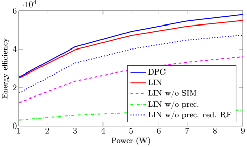
Next, we study how the EE varies with the maximum transmit power, as shown in Fig. 5. The EE curves for all schemes exhibit an approximately logarithmic shape due to the logarithmic increase in the achievable rate. As expected, the proposed schemes achieve higher EE compared to benchmark schemes. Among all the benchmark schemes, the LIN w/o prec. red. RF scheme obtains the largest EE because of a smaller number of RF chains used. The difference between the EE of the proposed scheme with linear precoding scheme and that of any other benchmark scheme generally increases with transmit power, although these differences are almost stabilized at higher transmit power levels. Additionally, the DPC-based scheme consistently shows a noticeable improvement in EE over all other schemes, which can be attributed to the superior interference suppression capabilities of DPC.

In order to better understand the impact of realistic imperfections, we present the EE of the proposed schemes for the case of discrete SIM phase shifts in Fig. 6. The EE generally deteriorates as the number of quantization bits decreases. This effect is more evident for SIMs with a larger number of layers, since they contain more meta-elements and thus can cause a larger EE reduction. As a rule of thumb, at least 3 bits per meta-element are required for SIMs with a small $L$ (e.g., 2 or 4) to ensure that the EE reduction caused by quantization errors remains within acceptable limits. For SIMs with a larger $L$ , the minimum number of bits per meta-element is expected to be higher.

The per-iteration computational complexity of the proposed optimization schemes are shown in Table I. The relevant iteration counts for Dinkelbach’s method $I_{U}$ and $I_{X}$ , and the number of the line search steps, $I_{\phi,D}$ and $I_{\phi,L}$ , are averaged over the number of iterations required for each optimization scheme to reach 95 % of the EE at the 1000-th iteration. It can be observed that the number of iterations of Dinkelbach’s method remains almost unchanged as $K$ varies for both schemes, and the same holds true for the number of line search steps. Moreover, the computational complexity of the proposed optimization scheme for DPC-based systems is higher than that of the scheme with linear precoding when $K$ is 4 and 8. However, when $K$ increases to 12, the DPC-based scheme exhibits significantly lower complexity compared to the linear precoding scheme. This substantial increase in the complexity of the linear precoding scheme is due to the fact that the complexity of the precoding matrix optimization, $C_{x}$ , is proportional to $N_{t}$ when $K=12$ .

	DPC			Linear precoding
$K$	$I_{U}$	$I_{\phi,D}$	$C_{\text{DPC}}$	$I_{X}$	$I_{\phi,L}$	$C_{\text{LIN}}$
4	55	1	4367616	51	1	4129024
8	55	1	4480256	50	1	4409600
12	55	1	4592896	51	1	9947392

TABLE I: Comparison of the per-iteration computational complexities of the schemes with DPC and linear precoding.

VIII Conclusion

In this paper, we studied the EE maximization in a SIM-aided broadcast system with DPC and linear precoding at the BS. For DPC, we exploited the well-known BC-MAC duality and optimize the users’ covariance matrices by employing a SCA-based technique, which establishes a tight lower bound of the achievable sum-rate, and applying Dinkelbach’s method. A similar approach was used to optimize the precoders in the case of linear precoding. The phase shifts of the SIM meta-elements for DPC and linear precoding were optimized using a conventional projected gradient-based method due to its simplicity. Also, we conducted a computation complexity analysis of the proposed optimization algorithms and proved their convergence. Numerical results showed that implementing these proposed optimization algorithms can significantly improve the EE for SIM-aided broadcast systems. Moreover, we demonstrated that the EE depends on the number of SIM meta-elements and their distribution across the SIM layers. We also found that in SIM-aided broadcast systems without precoding, optimal energy efficient transmission strategies typically involve a subset of active transmit antennas.

Appendix A Proof of Theorem 2

Differentiating $R_{k}(\boldsymbol{\phi})$ in (56) w.r.t. $\mathbf{H}_{k}$ yields

\text{d}R_{\text{L},k}(\boldsymbol{\phi})=\text{d}\ln\left|\mathbf{F}_{1,k}\right|-\text{d}\ln\left|\mathbf{F}_{2,k}\right|

(66)

where

	$\displaystyle\text{d}\ln\left\|\mathbf{F}_{1,k}\right\|$	$\displaystyle=\operatorname{Tr}\left(\hat{\mathbf{P}}_{s}\mathbf{H}_{k}^{H}\mathbf{F}_{1,k}^{-1}\text{d}\mathbf{H}_{k}+\mathbf{F}_{1,k}^{-1}\mathbf{H}_{k}\hat{\mathbf{P}}_{s}\text{d}\mathbf{H}_{k}^{H}\right)$		(67)
	$\displaystyle\!\!\!\text{d}\ln\left\|\mathbf{F}_{2,k}\right\|$	$\displaystyle=\operatorname{Tr}\left(\hat{\mathbf{P}}_{s}\mathbf{H}_{k}^{H}\mathbf{F}_{2,k}^{-1}\text{d}\mathbf{H}_{k}+\mathbf{F}_{2,k}^{-1}\mathbf{H}_{k}\hat{\mathbf{P}}_{k}\text{d}\mathbf{H}_{k}^{H}\right).$		(68)

Substituting (40) into the previous expressions, we obtain

	$\displaystyle\text{d}\ln\left\|\mathbf{F}_{1,k}\right\|$	$\displaystyle=\operatorname{Tr}\left(\mathbf{G}_{1}^{H}\text{d}\boldsymbol{\mathbf{\Phi}}^{l}+\mathbf{G}_{1}\text{d}(\boldsymbol{\mathbf{\Phi}}^{l})^{H}\right)$		(69)
	$\displaystyle\text{d}\ln\left\|\mathbf{F}_{2,k}\right\|$	$\displaystyle=\operatorname{Tr}\left(\mathbf{G}_{2}^{H}\text{d}\boldsymbol{\mathbf{\Phi}}^{l}+\mathbf{G}_{2}\text{d}(\boldsymbol{\mathbf{\Phi}}^{l})^{H}\right)$		(70)

where

	$\displaystyle\mathbf{G}_{1}=$	$\displaystyle\boldsymbol{\Theta}^{l+1:L}\mathbf{G}_{k}^{H}\mathbf{F}_{1}^{-1}\mathbf{H}_{k}\hat{\mathbf{P}}_{s}\boldsymbol{\Theta}^{1:l-1}\mathbf{W}_{l}^{H}$		(71)
	$\displaystyle\mathbf{G}_{2}=$	$\displaystyle\boldsymbol{\Theta}^{l+1:L}\mathbf{G}_{k}^{H}\mathbf{F}_{2}^{-1}\mathbf{H}_{k}\hat{\mathbf{P}}_{k}\boldsymbol{\Theta}^{1:l-1}\mathbf{W}_{l}^{H}$		(72)

After a few simple mathematical steps, we get

	$\displaystyle\nabla_{\boldsymbol{\phi}^{l}}R_{\text{L},k}(\boldsymbol{\phi})=\operatorname{vec}_{d}\left(\boldsymbol{\Theta}^{l+1:L}\mathbf{G}_{k}^{H}\mathbf{F}_{1,k}^{-1}\mathbf{H}_{k}\hat{\mathbf{P}}_{s}\boldsymbol{\Theta}^{1:l-1}\mathbf{W}_{l}^{H}\right)$
	$\displaystyle-\operatorname{vec}_{d}\left(\boldsymbol{\Theta}^{l+1:L}\mathbf{G}_{k}^{H}\mathbf{F}_{2,k}^{-1}\mathbf{H}_{k}\hat{\mathbf{P}}_{k}\boldsymbol{\Theta}^{1:l-1}\mathbf{W}_{l}^{H}\right).$		(73)

From this gradient expression for the achievable rate of user $k$ , we can easily obtain the appropriate gradients for all other users. After summation of all these gradient expressions, we obtain (58). This completes the proof.

References

[1] “Framework and overall objectives of the future development of imt for 2030 and beyond,” International Telecommunication Union (ITU) Recommendation (ITU-R), 2023.
[2] “Mobile data traffic outlook – Ericsson Mobility Report,” 2024, [Accessed 05-07-2024]. [Online]. Available: https://www.ericsson.com/en/reports-and-papers/mobility-report/dataforecasts/mobile-traffic-forecast
[3] M. Di Renzo et al., “Smart radio environments empowered by reconfigurable intelligent surfaces: How it works, state of research, and the road ahead,” IEEE Journal on Selected Areas in Communications, vol. 38, no. 11, pp. 2450–2525, 2020.
[4] T. Gong et al., “Holographic MIMO communications: Theoretical foundations, enabling technologies, and future directions,” IEEE Communications Surveys & Tutorials, vol. 26, no. 1, pp. 196–257, 2024.
[5] A. Zappone et al., “Energy efficiency of holographic transceivers based on RIS,” in GLOBECOM 2022-2022 IEEE Global Communications Conference. IEEE, 2022, pp. 4613–4618.
[6] N. Shlezinger et al., “Dynamic metasurface antennas for 6G extreme massive MIMO communications,” IEEE Wireless Communications, vol. 28, no. 2, pp. 106–113, 2021.
[7] L. You et al., “Energy efficiency maximization of massive MIMO communications with dynamic metasurface antennas,” IEEE Transactions on Wireless Communications, vol. 22, no. 1, pp. 393–407, 2022.
[8] C. Liu et al., “A programmable diffractive deep neural network based on a digital-coding metasurface array,” Nature Electronics, vol. 5, no. 2, pp. 113–122, 2022.
[9] J. An et al., “Two-dimensional direction-of-arrival estimation using stacked intelligent metasurfaces,” arXiv preprint arXiv:2402.08224, 2024.
[10] Q.-U.-A. Nadeem et al., “Hybrid digital-wave domain channel estimator for stacked intelligent metasurface enabled multi-user MISO systems,” arXiv preprint arXiv:2309.16204, 2023.
[11] Z. Wang et al., “Multi-user ISAC through stacked intelligent metasurfaces: New algorithms and experiments,” arXiv preprint arXiv:2405.01104, 2024.
[12] N. U. Hassan et al., “Efficient beamforming and radiation pattern control using stacked intelligent metasurfaces,” IEEE Open Journal of the Communications Society, vol. 5, pp. 599–611, 2024.
[13] J. An et al., “Stacked intelligent metasurfaces for multiuser downlink beamforming in the wave domain,” arXiv preprint arXiv:2309.02687, 2023.
[14] A. Papazafeiropoulos et al., “Achievable rate optimization for large stacked intelligent metasurfaces based on statistical CSI,” IEEE Wireless Communications Letters, 2024, Early Access.
[15] S. Lin et al., “Stacked intelligent metasurface enabled LEO satellite communications relying on statistical CSI,” IEEE Wireless Communications Letters, vol. 13, no. 5, pp. 1295–1299, 2024.
[16] H. Liu et al., “DRL-based orchestration of multi-user MISO systems with stacked intelligent metasurfaces,” arXiv preprint arXiv:2402.09006, 2024.
[17] Q. Li et al., “Stacked intelligent metasurfaces for holographic MIMO aided cell-free networks,” IEEE Transactions on Communications, 2024, Early Access.
[18] J. An et al., “Stacked intelligent metasurfaces for efficient holographic MIMO communications in 6G,” IEEE Journal on Selected Areas in Communications, vol. 41, no. 8, pp. 2380–2396, 2023.
[19] A. Papazafeiropoulos et al., “Achievable rate optimization for stacked intelligent metasurface-assisted holographic MIMO communications,” arXiv preprint arXiv:2402.16415, 2024.
[20] N. S. Perović and L.-N. Tran, “Mutual information optimization for SIM-based holographic MIMO systems,” arXiv preprint arXiv:2403.18307, 2024.
[21] X. Lin et al., “All-optical machine learning using diffractive deep neural networks,” Science, vol. 361, no. 6406, pp. 1004–1008, 2018.
[22] S. Vishwanath et al., “Duality, achievable rates, and sum-rate capacity of gaussian MIMO broadcast channels,” IEEE Transactions on Information Theory, vol. 49, no. 10, pp. 2658–2668, 2003.
[23] J. Xu and L. Qiu, “Energy efficiency optimization for MIMO broadcast channels,” IEEE Transactions on Wireless Communications, vol. 12, no. 2, pp. 690–701, 2013.
[24] H. H. M. Tam et al., “Successive convex quadratic programming for quality-of-service management in full-duplex MU-MIMO multicell networks,” IEEE Transactions on Communications, vol. 64, no. 6, pp. 2340–2353, 2016.
[25] N. S. Perović et al., “On the maximum achievable sum-rate of the ris-aided mimo broadcast channel,” IEEE Transactions on Signal Processing, vol. 70, pp. 6316–6331, 2022.
[26] X. Zhao et al., “Rethinking WMMSE: Can its complexity scale linearly with the number of BS antennas?” IEEE Transactions on Signal Processing, vol. 71, pp. 433–446, 2023.
[27] S. He et al., “Coordinated beamforming for energy efficient transmission in multicell multiuser systems,” IEEE Transactions on Communications, vol. 61, no. 12, pp. 4961–4971, 2013.
[28] J. Wang et al., “Reconfigurable intelligent surface: Power consumption modeling and practical measurement validation,” IEEE Transactions on Communications, 2024, Early Access.
[29] C. Huang et al., “Reconfigurable intelligent surfaces for energy efficiency in wireless communication,” IEEE Transactions on Wireless Communications, vol. 18, no. 8, pp. 4157–4170, 2019.