Energy-Based Generative Cooperative Saliency Prediction
Abstract
Conventional saliency prediction models typically learn a deterministic mapping from an image to its saliency map, and thus fail to explain the subjective nature of human attention. In this paper, to model the uncertainty of visual saliency, we study the saliency prediction problem from the perspective of generative models by learning a conditional probability distribution over the saliency map given an input image, and treating the saliency prediction as a sampling process from the learned distribution. Specifically, we propose a generative cooperative saliency prediction framework, where a conditional latent variable model (LVM) and a conditional energy-based model (EBM) are jointly trained to predict salient objects in a cooperative manner. The LVM serves as a fast but coarse predictor to efficiently produce an initial saliency map, which is then refined by the iterative Langevin revision of the EBM that serves as a slow but fine predictor. Such a coarse-to-fine cooperative saliency prediction strategy offers the best of both worlds. Moreover, we propose a “cooperative learning while recovering” strategy and apply it to weakly supervised saliency prediction, where saliency annotations of training images are partially observed. Lastly, we find that the learned energy function in the EBM can serve as a refinement module that can refine the results of other pre-trained saliency prediction models. Experimental results show that our model can produce a set of diverse and plausible saliency maps of an image, and obtain state-of-the-art performance in both fully supervised and weakly supervised saliency prediction tasks.
1 Introduction
As a class-agnostic segmentation task, salient object detection has attracted a lot of attentions in the computer vision community for its close relationship to human visual perception. A salient region is a visually distinctive scene region that can be located rapidly and with little human effort. Salient object detection is commonly treated as a pixel-wise binary output of a deterministic prediction model in most recent works (Wu, Su, and Huang 2019a; Qin et al. 2019; Wu, Su, and Huang 2019b; Wei, Wang, and Huang 2020; Wang et al. 2019; Xu et al. 2021). Despite the success of those recent models, the one-to-one deterministic mapping has prevented them from modeling the uncertainty of human salient object prediction, which is considered to be subjective (Itti, Koch, and Niebur 1998) and affected by biological factors (e.g., contrast sensitivity), contextual factors (e.g., task, experience, and interest), etc. In this way, it is more reasonable to represent visual saliency as a conditional probability distribution over a saliency map given an input image, and formulate the saliency prediction as a stochastic sampling process from the conditional distribution.
Generative models (Goodfellow et al. 2014; Kingma and Welling 2013; Xie et al. 2016, 2018a) have demonstrated their abilities to represent conditional distributions of high-dimensional data and produce multiple plausible outputs given the same input (Zhu et al. 2017; Xie et al. 2021b). In this work, we fit the saliency detection task into a generative framework, where the input image is the condition, and the goal is to generate multiple saliency maps, representing the “subjective nature” of human visual saliency. Zhang et al. (2020a, 2021) have used conditional variational auto-encoders (VAEs) (Kingma and Welling 2013; Sohn, Lee, and Yan 2015a), which are latent variable models (LVMs), to implicitly represent distributions of visual saliency. However, VAEs only learn a stochastic mapping from image domain to saliency domain, and lack an intrinsic cost function to evaluate the visual saliency output and guide the saliency prediction process. As to a prediction task, a cost function of solution is more reliable than a mapping function because the former is more generalizable than the latter.
In contrast, we propose to model the conditional distribution of visual saliency explicitly via an energy-based model (EBM) (Xie et al. 2016; Nijkamp et al. 2019), where the energy function defined on both image and saliency domains serves as a cost function of the saliency prediction. Given an input image, the saliency prediction can be achieved by performing sampling from the EBM via Markov chain Monte Carlo (MCMC) (Neal 2012) method, which is a gradient-based algorithm that searches local minima of the cost function of the EBM conditioned on the input image.
A typical high-dimensional EBM learns an energy function by MCMC-based maximum likelihood estimation (MLE), which commonly suffers from convergence difficulty and computational expensiveness of the MCMC process. Inspired by prior success of energy-based generative cooperative learning (Xie et al. 2018a, 2021b), we propose the energy-based generative cooperative saliency prediction framework to tackle the saliency prediction task. Specifically, the framework consists of a conditional EBM whose energy function is parameterized by a bottom-top neural network, and a conditional LVM whose transformation function is parameterized by an encoder-decoder framework. The framework brings in an LVM as an ancestral sampler to initialize the MCMC computational process of the EBM for efficient sampling, so that the EBM can be learned efficiently. The EBM, in turn, refines the LVM’s generated samples via MCMC and feeds them back to the LVM, so that the LVM can learn its mapping function from the MCMC transition. Thus, the resulting cooperative saliency prediction process first generates an initial saliency map via a direct mapping and then refines the saliency map via an iterative process. This is a coarse-to-fine generative saliency detection, and corresponds to a fast-thinking and slow-thinking system (Xie et al. 2021b).
Moreover, based on the generative cooperative saliency prediction framework, we further propose a cooperative learning while cooperative recovering strategy for weakly supervised saliency learning, where each training image is associated with a partially observed annotation (e.g., scribble annotation (Zhang et al. 2020b)). At each learning iteration, the strategy has two sub-tasks: cooperative recovery and cooperative learning. As to the cooperative recovery sub-task, each incomplete saliency ground truth is firstly recovered in the low-dimensional latent space of the LVM via inference, and then refined by being pushed to the local mode of the cost landscape of the EBM via MCMC. For the cooperative learning sub-task, the recovered saliency maps are treated as pseudo labels to update the parameters of the framework as in the scenario of learning from complete data.
In experiments, we demonstrate that our framework can not only achieve state-of-the-art performances in both fully supervised and weakly supervised saliency predictions, but also generate diverse saliency maps from one input image, indicating the success of modeling the uncertainty of saliency prediction. Furthermore, we show that the learned energy function in the EBM can serve as a cost function, which is useful to refine the results from other pre-trained saliency prediction models.
Our contributions can be summarized as below:
-
•
We study generative modeling of saliency prediction, and formulate it as a sampling process from a probabilistic model using EBM and LVM respectively, which are new angles to model and solve saliency prediction.
-
•
We propose a generative cooperative saliency prediction framework, which jointly trains the LVM predictor and the EBM predictor in a cooperative learning scheme to offer reliable and efficient saliency prediction.
-
•
We generalize our generative framework to the weakly supervised saliency prediction scenario, in which only incomplete annotations are provided, by proposing the cooperative learning while recovering algorithm, where we train the model and simultaneously recover the unlabeled areas of the incomplete saliency maps.
-
•
We provide strong empirical results in both fully supevised and weakly supervised settings to verify the effectiveness of our framework for saliency prediction.
2 Related Work
We first briefly introduce existing fully supervised and weakly supervised saliency prediction models. We then review the family of generative cooperative models and other conditional deep generative frameworks.
Fully Supervised Saliency Prediction. Existing fully supervised saliency prediction models (Wang et al. 2018; Liu, Han, and Yang 2018; Wei, Wang, and Huang 2020; Liu et al. 2019; Qin et al. 2019; Wu, Su, and Huang 2019b, a; Wang et al. 2019, 2019; Wei et al. 2020; Xu et al. 2021) mainly focus on exploring image context information and generating structure-preserving predictions.Wu, Su, and Huang (2019b); Wang et al. (2019, 2019, 2018); Liu, Han, and Yang (2018); Liu et al. (2019); Wu, Su, and Huang (2019a); Xu et al. (2021) propose saliency prediction models by effectively integrating higher-level and lower-level features. Wei, Wang, and Huang (2020); Wei et al. (2020) propose an edge-aware loss term to penalize errors along object boundaries.Zhang et al. (2020a) present a stochastic RGB-D saliency detection network based on the conditional variational auto-encoder (Kingma and Welling 2013; Jimenez Rezende, Mohamed, and Wierstra 2014). In this paper, we introduce the conditional cooperative learning framework (Xie et al. 2018a, 2021b) to achieve probabilistic coarse-to-fine RGB saliency detection, where a coarse prediction is produced by a conditional latent variable model and then is refined by a conditional energy-based model. Our paper is the first work to use a deep energy-based generative framework for probabilistic saliency detection.
Weakly Supervised Saliency Prediction. Weakly supervised saliency prediction frameworks (Wang et al. 2017; Li, Xie, and Lin 2018a; Nguyen et al. 2019; Zhang et al. 2020b) attempt to learn predictive models from easy-to-obtain weak labels, including image-level labels (Wang et al. 2017; Li, Xie, and Lin 2018b), noisy labels (Nguyen et al. 2019; Zhang et al. 2018; Zhang, Han, and Zhang 2017) or scribble labels (Zhang et al. 2020b). In this paper, we also propose a cooperative learning while recovering strategy for weakly supervised saliency prediction, in which only scribble labels are provided and our model treats them as incomplete data and recovers them during learning.
Energy-Based Generative Cooperative Networks. Deep energy-based generative models (Xie et al. 2016), with energy functions parameterized by modern convolutional neural networks, are capable of modeling the probability density of high-dimensional data. They have been applied to image generation (Xie et al. 2016; Gao et al. 2018; Nijkamp et al. 2019; Du and Mordatch 2019; Grathwohl et al. 2020; Zhao, Xie, and Li 2021; Zheng, Xie, and Li 2021), video generation (Xie, Zhu, and Wu 2019), 3D volumetric shape generation (Xie et al. 2018b, 2020), and unordered point cloud generation (Xie et al. 2021a). The maximum likelihood learning of the energy-based model typically requires iterative MCMC sampling, which is computationally challenging. To relieve the computational burden of MCMC, the Generative Cooperative Networks (CoopNets) in Xie et al. (2018a) propose to learn a separate latent variable model (i.e. a generator) to serve as an efficient approximate sampler for training the energy-based model. Xie, Zheng, and Li (2021) propose a variant of CoopNets by replacing the generator with a variational auto-encoder (VAE) (Kingma and Welling 2014). Xie et al. (2021b) propose a conditional CoopNets for supervised image-to-image translation. Our paper proposes a conditional CoopNets for visual saliency prediction. Further, we generalize our model to the weakly supervised learning scenario by proposing a cooperative learning while recovering algorithm. In this way, we can learn from incomplete data for weakly supervised saliency prediction.
Conditional Deep Generative Models. Our framework belongs to the family of conditional generative models, which include conditional generative adversarial networks (CGANs) (Mirza and Osindero 2014) and conditional variational auto-encoders (CVAEs) (Sohn, Lee, and Yan 2015a). Different from existing CGANs (Luc et al. 2016; Zhang et al. 2018; Xue et al. 2017; Pan et al. 2017; Yu and Cai 2018; Hung et al. 2018; Souly, Spampinato, and Shah 2017), which train a conditional discriminator and a conditional generator in an adversarial manner, or CVAEs (Kohl et al. 2018; Zhang et al. 2020a, 2021), in which a conditional generator is trained with an approximate inference network, our model learns a conditional generator with a conditional energy-based model via MCMC teaching. Specifically, our model allows an additional refinement for the generator during prediction, which is lacking in both CGANs and CVAEs.
3 Cooperative Saliency Prediction
We will first present two types of generative modeling of saliecny prediction, i.e., the energy-based model (EBM) and the latent variable model (LVM). Then, we propose a novel generative saliency prediction framework, in which the EBM and the LVM are jointly trained in a generative cooperative manner, such that they can help each other for better saliency prediction in terms of computational efficiency and prediction accuracy. The latter aims to generate a coarse but fast prediction, and the former serves as a fine saliency predictor. The resulting model is a coarse-to-fine saliency prediction framework.
3.1 EBM as a Slow but Fine Predictor
Let be an image, and be its saliency map. The EBM defines a conditional distribution of given by:
| (1) |
where the energy function , parameterized by a bottom-up neural network, maps the input image-saliency pair to a scalar, and represent the network parameters. is the normalizing constant. When is learned and an image is given, the prediction of saliency can be achieved by Langevin sampling (Neal 2012), which makes use of the gradient of the energy function and iterates the following step:
| (2) |
where indexes the Langevin time step, is the step size, and is a Gaussian noise term. The Langevin dynamics (Neal 2012) is initialized with Gaussian distribution and is equivalent to a stochastic gradient descent algorithm that seeks to find the minimum of the objective function defined by . The noise term is a Brownian motion that prevents gradient descent from being trapped by local minima of . The energy function in Eq. (1) can be regarded as a trainable cost function of the task of saliency prediction. The prediction process via Langevin dynamics in Eq. (2) can be considered as finding to minimize the cost given an input . Such a framework can learn a reliable and generalizable cost function for saliency prediction. However, due to the iterative sampling process in the prediction, EBM is slower than LVM, which adopts a mapping for direct sampling.
3.2 LVM as a Fast but Coarse Predictor
Let be a latent Gaussian noise vector. The LVM defines a mapping function that maps a latent vector together with an image to a saliency map . is a -dimensional identity matrix. is the number of dimensionalities of . Specifically, the mapping function is parameterized by a noise-injected encoder-decoder network with skip connections and contain all the learning parameters in the network. The LVM is given by:
| (3) |
where is an observation residual and is a predefined standard deviation of . The LVM in Eq. (3) defines an implicit conditional distribution of saliency given an image , i.e., , where . The saliency prediction can be achieved by an ancestral sampling process that first samples a Gaussian white noise vector and then transforms it along with an image to a saliency map . Since the ancestral sampling is a direct mapping, it is faster than the iterative Langevin dynamics in the EBM. However, without a cost function as in the EBM, the learned mapping in the LVM is hard to be generalized to a new domain.
3.3 Cooperative Prediction with Two Predictors
We propose to predict image saliency by a cooperative sampling strategy. We first use the coarse saliency predictor (LVM) to generate an initial prediction via a non-iterative ancestral sampling, and then we use the fine saliency predictor (EBM) to refine the initial prediction via -step Langevin revision to obtain a revised saliency . The process can be written as:
| (4) |
We call this process the cooperative sampling-based coarse-to-fine prediction. In this way, we take both advantages of these two saliency predictors in the sense that the fine saliency predictor (i.e., Langevin sampler) is initialized by the efficient coarse saliency predictor (i.e., ancestral sampler), while the coarse saliency predictor is refined by the accurate fine saliency predictor that aims to minimize a cost function .
Since our conditional model represents a one-to-many mapping, the prediction is stochastic. To evaluate the learned model on saliency prediction tasks, we can draw multiple from the prior and use their average to generate , then a Langevin dynamics with the diffusion term being disabled (i.e., gradient descent) is performed to push to its nearest local minimum based on the learned energy function. The resulting is treated as a prediction of our model.
3.4 Cooperative Training of Two Predictors
We use the cooperative training method (Xie et al. 2018a, 2021b) to learn the parameters of the two predictors. At each iteration, we first generate synthetic examples via the cooperative sampling strategy shown in Eq. (4), and then the synthetic examples are used to compute the learning gradients to update both predictors. We present the update formula of each predictor below.
MCMC-based Maximum Likelihood Estimation (MLE) for the Fine Saliency Predictor. Given a training dataset , we train the fine saliency predictor via MLE, which maximizes the log-likelihood of the data , whose learning gradient is . We rely on the cooperative sampling in Eq. (4) to sample to approximate the gradient:
| (5) |
We can use Adam (Kingma and Ba 2015) with to update . We denote as a function of and .
Maximum Likelihood Training of the Coarse Saliency Predictor by MCMC Teaching. Even though the fine saliency predictor learns from the training data, the coarse saliency predictor learns to catch up with the fine saliency predictor by treating as training examples. The learning objective is to maximize the log-likelihood of the samples drawn from , i.e., , whose gradient can be computed by
| (6) |
This leads to an MCMC-based solution that iterates (i) an inference step: inferring latent by sampling from posterior distribution via Langevin dynamics, which iterates the following:
| (7) |
where and , and (ii) a learning step: with , we update via Adam optimizer with
| (8) |
Since is parameterized by a differentiable neural network, both in Eq. (7) and in Eq. (8) can be efficiently computed by back-propagation. We denote as a function of and . Algorithm 1 presents a description of the cooperative learning algorithm of the fine and coarse saliency predictors.
Input:
(1) Training images with associated saliency maps ;
(2) maximal number of learning iterations .
Output: Parameters and
4 Weakly Supervised Saliency Prediction
In Section 3, the framework is trained from fully-observed training data. In this section, we want to show that our generative framework can be modified to handle the scenario in which each image only has a partial pixel-wise annotation , e.g., scribble annotation (Zhang et al. 2020b). Since the saliency map for each training image is incomplete, directly applying the algorithm to the incomplete training data can lead to a failure of learning the distribution of saliency given an image. However, generative models are good at data recovery, therefore they can learn to recover the incomplete data. In our framework, we will leverage the recovery powers of both EBM and LVM to deal with the incomplete data in our cooperative learning algorithm, and this will lead to a novel weakly supervised saliency prediction framework.
To learn from incomplete data, our algorithm alternates the cooperative learning step and the cooperative recovery step. Both steps need a cooperation between EBM and LVM. The cooperative learning step is the same as the one used for fully observed data, except that it treats the recovered saliency maps, which are generated from the cooperative recovery step, as training data in each iteration. The following is the cooperative recovery step, which consists of two sub-steps driven by the LVM and the EBM respectively:
(i) Recovery by LVM in Latent Space. Given an image and its incomplete saliency map , the recovery of the missing part of can be achieved by first inferring the latent vector based on the partially observed saliency information via , and then generating with the inferred latent vector . Let be a binary mask, with the same size as , indicating the locations of visible annotations in . varies for different and can be extracted from . The Langevin dynamics for recovery iterates the same step in Eq. (7) except that , where denotes element-wise matrix multiplication operation.
(ii) Recovery by EBM in Data Space. With the initial recovered result generated by the coarse saliency predictor , the fine saliency predictor can further refine the result by running a finite-step Langevin dynamics, which is initialized with , to obtain . The underlying principle is that the initial recovery might be just around one local mode of the energy function. A few steps of Langevin dynamics (i.e., stochastic gradient descent) toward , starting from , will push to its nearby low energy mode, which might correspond to its complete version .
Input:
(1) Images with incomplete annotations ;
(2) Number of learning iterations
Output: Parameters and
Cooperative Learning and Recovering. At each iteration , we perform the above cooperative recovery of the incomplete saliency maps via and , while learning and from , where are the recovered saliency maps at iteration . The parameters are still updated via Eq. (5) except that we replace by . That is, at each iteration, we use the recovered , as well as the synthesized , to compute the gradient of the log-likelihood, which is denoted by . The algorithm simultaneously performs (i) cooperative recovering of missing annotations of each training example; (ii) cooperative sampling to generate annotations; (iii) cooperative learning of the two models by updating parameters with both recovered annotations and generated annotations. See Algorithm 2 for a detailed description of the learning while recovering algorithm.
5 Technical Details
We present the details of architecture designs of the LVM and the EBM, as well as the hyper-parameters below.
Latent Variable Model: The LVM , using the ResNet50 (He et al. 2016) as an encoder backbone, maps an image and a latent vector to a saliency map . Specifically, we adopt the decoder from the MiDaS (Ranftl et al. 2020) for its simplicity, which gradually aggregates the higher level features with lower level features via residual connections. We introduce the latent vector to the bottleneck of the LVM by concatenating the tiled with the highest level features of the encoder backbone, and then feed them to a convolutional layer to obtain a feature map with the same size as the original highest level feature map of the encoder. The latent-vector-aware feature map is then fed to the decoder from Ranftl et al. (2020) to generate a final saliency map. As shown in Eq. (8), the parameters of the LVM are updated with the revised predictions provided by the EBM. Thus, immature in the early stage of the cooperative learning might bring in fluctuation in training the LVM, which in turn affects the convergence of the MCMC samples . To stabilize the cooperative training, especially in the early stage, we let the LVM learn from not only but also . Specifically, we add an extra loss for the LVM as , where linearly decreases to 0 during training, and is the cross-entropy loss.
Energy-Based Model: The energy function is parameterized by a neural network that maps the channel-wise concatenation of and to a scalar. Let cksl-n denote a kk Convolution-BatchNorm-ReLU layer with n filters and a stride of l. Let fc-n be a fully connected layer with n filters. The is our framework consists of the following layers: c3s1-32, c4s2-64, c4s2-128, c4s2-256, c4s1-1, fc-100.
| DUTS | ECSSD | DUT | HKU-IS | PASCAL-S | SOD | |||||||||||||||||||||
| Method | Year | BkB | ||||||||||||||||||||||||
| Fully Supervised Models | ||||||||||||||||||||||||||
| PoolNet | 2019 | R50 | .887 | .840 | .910 | .037 | .919 | .913 | .938 | .038 | .831 | .748 | .848 | .054 | .919 | .903 | .945 | .030 | .865 | .835 | .896 | .065 | .820 | .804 | .834 | .084 |
| BASNet | 2019 | R34 | .876 | .823 | .896 | .048 | .910 | .913 | .938 | .040 | .836 | .767 | .865 | .057 | .909 | .903 | .943 | .032 | .838 | .818 | .879 | .076 | .798 | .792 | .827 | .094 |
| SCRN | 2019 | R50 | .885 | .833 | .900 | .040 | .920 | .910 | .933 | .041 | .837 | .749 | .847 | .056 | .916 | .894 | .935 | .034 | .869 | .833 | .892 | .063 | .817 | .790 | .829 | .087 |
| F3Net | 2020 | R50 | .888 | .852 | .920 | .035 | .919 | .921 | .943 | .036 | .839 | .766 | .864 | .053 | .917 | .910 | .952 | .028 | .861 | .835 | .898 | .062 | .824 | .814 | .850 | .077 |
| ITSD | 2020 | R50 | .885 | .840 | .913 | .041 | .919 | .917 | .941 | .037 | .840 | .768 | .865 | .061 | .917 | .904 | .947 | .031 | .860 | .830 | .894 | .066 | .836 | .829 | .867 | .076 |
| LDF | 2020 | R50 | .892 | .861 | .925 | .034 | .919 | .923 | .943 | .036 | .839 | .770 | .865 | .052 | .920 | .913 | .953 | .028 | .842 | .768 | .863 | .064 | - | - | - | - |
| UCNet+ | 2021 | R50 | .888 | .860 | .927 | .034 | .921 | .926 | .947 | .035 | .839 | .773 | .869 | .051 | .921 | .919 | .957 | .026 | .851 | .825 | .886 | .069 | .828 | .827 | .856 | .076 |
| PAKRN | 2021 | R50 | .900 | .876 | .935 | .033 | .928 | .930 | .951 | .032 | .853 | .796 | .888 | .050 | .923 | .919 | .955 | .028 | .858 | .838 | .896 | .067 | .833 | .836 | .866 | .074 |
| Our_F | 2021 | R50 | .902 | .877 | .936 | .032 | .928 | .935 | .955 | .030 | .857 | .798 | .889 | .049 | .927 | .917 | .960 | .026 | .873 | .846 | .909 | .058 | .854 | .850 | .885 | .064 |
| Weakly Supervised Models | ||||||||||||||||||||||||||
| SSAL | 2020 | R50 | .803 | .747 | .865 | .062 | .863 | .865 | .908 | .061 | .785 | .702 | .835 | .068 | .865 | .858 | .923 | .047 | .798 | .773 | .854 | .093 | .750 | .743 | .801 | .108 |
| SCWS | 2021 | R50 | .841 | .818 | .901 | .049 | .879 | .894 | .924 | .051 | .813 | .751 | .856 | .060 | .883 | .892 | .938 | .038 | .821 | .815 | .877 | .078 | .782 | .791 | .833 | .090 |
| Our_W | 2021 | R50 | .847 | .816 | .902 | .048 | .896 | .896 | .934 | .045 | .817 | .762 | .864 | .058 | .894 | .893 | .943 | .037 | .834 | .823 | .886 | .073 | .803 | .793 | .849 | .082 |
 |
 |
 |
 |
 |
 |
 |
 |
 |
 |
 |
 |
 |
 |
 |
 |
 |
 |
| Image | GT | SCRN | F3Net | ITSD | LDF | PAKRN | Ours_F | Uncertainty |
Implementation Details: We train our model with a maximum of 30 epochs. Each image is rescaled to . We set the number of dimensions of the latent space as . The number of Langevin steps is and the Langevin step sizes for EBM and LVM are 0.4 and 0.1. The learning rates of the LVM and EBM are initialized to and respectively. We use Adam optimizer with momentum 0.9 and decrease the learning rates by 10% after every 20 epochs. It takes 20 hours to train the model with a batch size of 7 using a single NVIDIA GeForce RTX 2080Ti GPU.
6 Experiments
We conduct a series of experiments to test the performances of the proposed generative cooperative frameworks for saliency prediction. We start from experiment setup.
Datasets: We use the DUTS dataset (Wang et al. 2017) to train the fully supervised model, and S-DUTS (Zhang et al. 2020b) dataset with scribble annotations to train the weakly supervised model. Testing images include (1) DUTS testing dataset, (2) ECSSD (Yan et al. 2013), (3) DUT (Yang et al. 2013), (4) HKU-IS (Li and Yu 2015), (5) PASCAL-S (Li et al. 2014) and (6)SOD dataset (Movahedi and Elder 2010).
Compared methods: We compare our method against state-of-the-art fully supervised saliency detection methods, e.g., PoolNet (Liu et al. 2019), BASNet (Qin et al. 2019), SCRN (Wu, Su, and Huang 2019b), F3Net (Wei, Wang, and Huang 2020), ITSD (Zhou et al. 2020), LDF (Wei et al. 2020), UCNet+ (Zhang et al. 2021) and PAKRN (Xu et al. 2021). UCNet+ (Zhang et al. 2021) is the only generative framework. We also compare our weakly supervised solution with the scribble saliency detection models, e.g., SSAL (Zhang et al. 2020b) and SCWS (Yu et al. 2021).
Evaluation Metrics: We evaluate performance of our models and compared methods with four saliency evaluation metrics, including Mean Absolute Error (), mean F-measure (), mean E-measure () (Fan et al. 2018) and S-measure () (Fan et al. 2017).
| DUTS | ECSSD | DUT | HKU-IS | PASCAL-S | SOD | |||||||||||||||||||
|---|---|---|---|---|---|---|---|---|---|---|---|---|---|---|---|---|---|---|---|---|---|---|---|---|
| EBM as Refinement Module | ||||||||||||||||||||||||
| BASN_R | .891 | .842 | .889 | .041 | .926 | .921 | .947 | .035 | .839 | .781 | .870 | .051 | .919 | .925 | .942 | .031 | .837 | .749 | .857 | .070 | .852 | .859 | .869 | .090 |
| SCRN_R | .899 | .857 | .923 | .034 | .920 | .921 | .938 | .037 | .831 | .748 | .854 | .053 | .921 | .919 | .958 | .027 | .857 | .769 | .871 | .062 | .857 | .867 | .873 | .080 |
| Ablation Study | ||||||||||||||||||||||||
| .878 | .835 | .918 | .038 | .916 | .915 | .946 | .036 | .826 | .751 | .862 | .058 | .912 | .901 | .952 | .030 | .856 | .830 | .899 | .064 | .829 | .827 | .871 | .072 | |
| .897 | .858 | .932 | .034 | .918 | .923 | .946 | .034 | .837 | .777 | .882 | .051 | .914 | .913 | .957 | .028 | .863 | .835 | .900 | .062 | .831 | .830 | .874 | .070 | |
| ITSD | .885 | .840 | .913 | .041 | .919 | .917 | .941 | .037 | .840 | .768 | .865 | .061 | .917 | .904 | .947 | .031 | .860 | .830 | .894 | .066 | .836 | .829 | .867 | .076 |
| ITSD_Ours | .914 | .880 | .945 | .030 | .938 | .935 | .959 | .029 | .860 | .803 | .901 | .044 | .933 | .927 | .971 | .026 | .875 | .848 | .921 | .055 | .845 | .835 | .880 | .067 |
| VGG16_Ours | .906 | .876 | .941 | .032 | .939 | .933 | .953 | .030 | .857 | .799 | .893 | .048 | .929 | .923 | .959 | .027 | .871 | .844 | .907 | .058 | .841 | .838 | .871 | .066 |
| Our_F | .902 | .877 | .936 | .032 | .928 | .935 | .955 | .030 | .857 | .798 | .889 | .049 | .927 | .917 | .960 | .026 | .873 | .846 | .909 | .058 | .854 | .850 | .885 | .064 |
 |
 |
 |
 |
 |
 |
 |
 |
 |
 |
 |
 |
| Image | GT | Scribble | Recovered |
6.1 Fully Supervised Saliency Prediction
We first test the performance of our fully supervised generative cooperative saliency prediction framework.
Quantitative comparison: We compare the performance of our models and the compared methods in Table 1, where “Ours_F” denotes the proposed fully supervised models. We observe consistent performance improvement of “Ours_F” over six testing datasets compared with benchmark models, which clearly shows the advantage of our model. Note that, we adopt an existing decoder structure, i.e., MiDaS decoder (Ranftl et al. 2020), for the latent variable model in our proposed framework due to its easy implementation. We conduct an ablation study in Section 6.4 to further investigate the design of the decoder. Since our model uses a stochastic method, i.e., cooperative sampling, for prediction, we report the mean prediction to evaluate the performance of our models. Also, we observe relatively stable performance for different samples of predictions in larger testing datasets, e.g., DUTS testing dataset (Wang et al. 2017), and slightly fluctuant performance in smaller testing datasets, e.g., SOD (Movahedi and Elder 2010) testing dataset.
 |
 |
 |
 |
 |
 |
 |
 |
 |
 |
 |
 |
 |
 |
 |
 |
 |
 |
 |
 |
 |
 |
 |
 |
| Image | GT | SSAL | SCWS | Ours_W | Uncer. |
Qualitative comparison: Figure 1 displays some qualitative results of the saliency predictions produced by our method and the compared methods. Each row corresponds to one example, and shows an input testing image, the corresponding ground truth saliency map, saliency maps predicted by SCRN, F3Net, ITSD, LDF and PAKRN, followed by the mean predicted saliency map and the pixel-wise uncertainty map of our model. The uncertainty map indicates the model confidence in predicting saliency from a given image, and is computed as the entropy (Kendall et al. 2017; Kendall and Gal 2017; Zhang et al. 2021, 2020a) of our model predictions. Results show that our method can not only produce visually reasonable saliency maps for input images but also meaningful uncertainty maps that are consistent with human perception.
Prediction time and model size comparison: We have two main modules in our framework, namely a latent variable model and an energy-based model. The former takes the ResNet50 (He et al. 2016) backbone as encoder, and the MiDaS (Ranftl et al. 2020) decoder for feature aggregation, leading to a model parameter size of 55M for the LVM. The latter adds 1M extra parameters to the cooperative learning framework. Thus, our model size is a total of 56M, which is comparable with mainstream saliency detection models, e.g., F3Net (Wei, Wang, and Huang 2020) has 48M parameters. As to the cooperative prediction time, it costs approximately 0.08 seconds to output a single prediction of saliency map, which is comparable with existing solutions as well.
6.2 Weakly Supervised Saliency Prediction
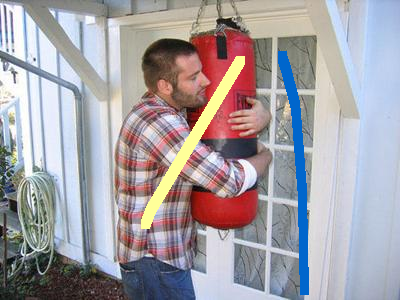
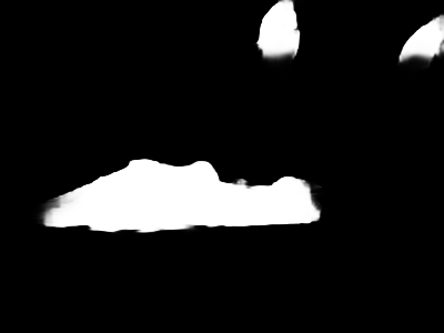
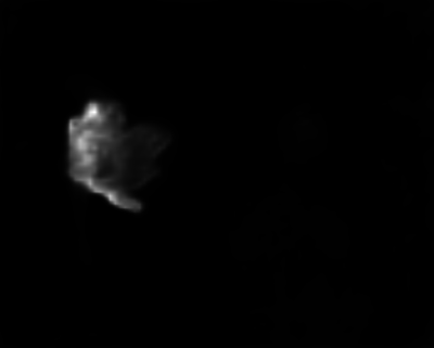
We then evaluate our weakly supervised generative cooperative saliency prediction framework on a dataset with scribble annotations (Zhang et al. 2020b), and show prediction performance on six testing sets in Table 1, where “Our_W” in the “Weakly Supervised Models” panel denotes our model. Figure 2 shows some examples of annotation recovery during training, where each row of example displays an input training image, the ground truth annotation as reference, scribble annotation used for training (the yellow scribble indicates the salient region, and the blue scribble indicates the background region), and the recovered saliency annotation obtained by our method. We compare our model with baseline methods, e.g., SSAL (Zhang et al. 2020b) and SCWS (Yu et al. 2021). The better performance of our model in testing shows the effectiveness of the proposed “cooperative learning while recovering” algorithm. Figure 3 displays a comparison of qualitative results obtained by different weakly supervised saliency prediction methods in testing.
6.3 Energy Function as a Refinement Module
As shown in Eq. (2), the EBM can iteratively refine the saliency prediction by Langevin sampling. With a well-trained energy function, we can treat it as a refinement module to refine predictions from existing saliency detection models. To demonstrate this idea, we select “BASN” (Qin et al. 2019) and “SCRN” (Wu, Su, and Huang 2019b) as base models due to the accessibility of their codes and predictions. We refine their predictions with the trained EBM and denote them by “BASN_R” and “SCRN_R”, respectively. Performances are shown in Table 2. Comparing with the performance of the base models in Table 1, we observe consistent performance improvements by using the trained EBM for refinement in Table 2. We show three examples of these models with and without EBM refinement in Figure 4. The qualitative improvement due to the usage of the EBM refinement verifies the usefulness of learned energy function.
 |
 |
 |
 |
 |
 |
 |
 |
 |
 |
 |
 |
 |
 |
 |
 |
 |
 |
| Image | GT | BASN | BASN_R | SCRN | SCRN_R |
6.4 Ablation Study
We conduct the following experiments as shown in Table 2 to further analyze our proposed framework. Training a deterministic noise-free encoder-decoder : We remove the latent vector from our noise-injected encoder-decoder and obtain a deterministic noise-free encoder-decoder . We train with the cross-entropy loss as in those conventional deterministic saliency prediction models. In comparison with the state-of-the-art deterministic saliency detection model, i.e., PAKRN (Xu et al. 2021), shows inferior performance due to its usage of a relatively small decoder (Ranftl et al. 2020). However, the superior performance of “Ours_F”, which is built upon that shares the same decoder structure with , has exhibited the usefulness of the latent vector for generative modeling and verified the effectiveness of the EBM for cooperative learning.
Training a latent variable model without the EBM: To further validate the importance of the cooperative training, we train a single latent variable model without relying on an EBM, which leads to the alternating back-propagation training scheme (Han et al. 2017). directly learns from observed training data rather than synthesized examples provided by an EBM. Compared with trained independently, ”Ours_F“ achieves better performance, which validates the effectiveness of the cooperative learning strategy.
| DUTS | ECSSD | DUT | HKU-IS | PASCAL-S | SOD | |||||||||||||||||||
|---|---|---|---|---|---|---|---|---|---|---|---|---|---|---|---|---|---|---|---|---|---|---|---|---|
| Method | ||||||||||||||||||||||||
| CVAE | .890 | .849 | .925 | .036 | .919 | .918 | .948 | .034 | .836 | .761 | .868 | .056 | .918 | .906 | .955 | .028 | .863 | .835 | .902 | .062 | .838 | .830 | .878 | .071 |
| CGAN | .888 | .849 | .927 | .035 | .917 | .914 | .944 | .036 | .837 | .764 | .871 | .054 | .917 | .908 | .955 | .028 | .865 | .839 | .906 | .059 | .836 | .833 | .874 | .072 |
| MCD | .881 | .842 | .918 | .038 | .917 | .917 | .944 | .036 | .828 | .753 | .859 | .057 | .915 | .908 | .951 | .030 | .863 | .837 | .902 | .062 | .834 | .831 | .868 | .073 |
| ENS | .885 | .841 | .921 | .037 | .921 | .917 | .948 | .035 | .831 | .752 | .862 | .057 | .916 | .901 | .952 | .030 | .858 | .827 | .897 | .065 | .835 | .828 | .872 | .073 |
| Our_F | .902 | .877 | .936 | .032 | .928 | .935 | .955 | .030 | .857 | .798 | .889 | .049 | .927 | .917 | .960 | .026 | .873 | .846 | .909 | .058 | .854 | .850 | .885 | .064 |
 |
Design of encoder and encoder structures: We replace the decoder part in our proposed framework by the one of those existing deterministic saliency prediction methods, e.g., ITSD (Zhou et al. 2020). We select ITSD (Zhou et al. 2020) because of the availability of its code and the state-of-the-art performance. We show its performance in Table 2 as “ITSD_Ours”. Further, we replace the ResNet50 (He et al. 2016) encoder backbone in our model by VGG16 (Simonyan and Zisserman 2014) and denote the new model as “VGG16_Ours”. The consistently better performance of “ITSD_Ours” than the original “ITSD” validates the superiority of the generative cooperative learning framework. Comparable performances are observed in our models with different backbone selections.
6.5 Alternative Uncertainty Estimation Methods
In this section, we compare our generative framework with other alternative uncertainty estimation methods for saliency prediction. We first design two alternatives based on CVAEs (Sohn, Lee, and Yan 2015b) and CGANs (Mirza and Osindero 2014), respectively. For the CVAE model, we follow Zhang et al. (2021), except that we replace its decoder network by our decoder (Ranftl et al. 2020). As to the CGAN, we optimize the adversarial loss (Goodfellow et al. 2014) of the conditional generative adversarial network that consists of a conditional generator and a conditional discriminator . Specifically, we use the same latent variable model as that in our model for the generator of CGAN. For the discriminator, we design a fully convolutional discriminator as in Hung et al. (2018) to classify each pixel into real (ground truth) or fake (prediction). To train CGAN, the discriminator is updated with the discriminator loss , where is the binary cross-entropy loss, and are all-one and all-zero maps of the same spatial size as . is updated with , where is the adversarial loss for and is the cross-entropy loss between the outputs of and the observed saliency maps. We set .
We also design two ensemble-based saliency detection frameworks with Monte Carlo dropout (Gal and Ghahramani 2016) and deep ensemble (Lakshminarayanan, Pritzel, and Blundell 2017) to produce multiple predictions, and show their performance as “MCD” and “ENS” in Table 3 respectively. For “MCD”, we add dropout to each level of features of the encoder within the noise-free encoder-decoder with a dropout rate 0.3, and use dropout in both of training and testing processes. For “ENS”, we attach five MiDaS decoder (Ranftl et al. 2020) to , which are initialized differently, leading to five outputs of predictions. For both ensemble-based frameworks, similar to our generative models, we use the mean prediction averaging over 10 samples in testing as the final prediction, and the entropy of the mean prediction as the predictive uncertainty following Skafte, Jø rgensen, and Hauberg (2019).
We show performance of alternative uncertainty estimation models in Table 3, and visualize the mean prediction and predictive uncertainty for each method in Figure 5. For the CVAE-based framework, designing the approximate inference network takes extra efforts, and the imbalanced inference model may lead to the posterior collapse issue as discussed in He et al. (2019). For the CGAN-based model, according to our experiments, the training is sensitive to the proportion of the adversarial loss. Further, it cannot infer the latent variables , which makes the model hard to learn from incomplete data for weakly supervised learning. For the deep ensemble (Lakshminarayanan, Pritzel, and Blundell 2017) and MC dropout (Gal and Ghahramani 2016) solutions, they can hardly improve model performance, although the produced predictive uncertainty maps can explain model prediction to some extent. Compared all above alternative methods, our proposed framework is stable due to maximum likelihood learning, and we can infer latent variables without the need of an extra encoder. Further, as we directly sample from the truth posterior distribution via Langevin dynamics, instead of the approximated inference network, we have more reliable and accurate predictive uncertainty maps compared with other alternative solutions.
7 Conclusion and Discussion
In this paper, we propose a novel energy-based generative saliency prediction framework based on the conditional generative cooperative network, where a conditional latent variable model and an conditional energy-based model are jointly trained in a cooperative learning scheme to achieve a coarse-to-fine saliency prediction. The latent variable model serves as a coarse saliency predictor that provides a fast initial saliency prediction, while the energy-based model serves as a fine saliency predictor that further refines the initial output by the Langevin revision. Even though each of the models can represent the conditional probability distribution of saliency, the cooperative representation and training can offer the best of both worlds. Moreover, we propose a cooperative learning while recovering strategy and apply the model to the weakly supervised saliency detection scenario, in which partial annotations (e.g., scribble annotations) are provided for training. As to the cooperative recovery part of the proposed strategy, the latent variable model serves as a fast but coarse saliency recoverer that provides an initial recovery of the missing annotations from the latent space via inference process, while the energy-based model serves as a slow but fine saliency recoverer that refines the initial recovery results by Langevin dynamics. Combining these two types of recovery schemes leads to a coarse-to-fine recoverer. Further, we find that the learned energy function in the energy-based model can serve as a refinement module, which can be easily plugged into the existing pre-trained saliency prediction models. The energy function is the potential cost function trained from the saliency prediction task. In comparison to a mapping function from image to saliency, the cost function captures the criterion to measure the quality of the saliency given an image, and is more generalizable so that it can be used to refine other saliency predictions. Extensive results exhibit that, compared with both conventional deterministic mapping methods and alternative uncertainty estimation methods, our framework can lead to both accurate saliency predictions for computer vision tasks and reliable uncertainty maps indicating the model confidence in performing saliency prediction from an image. As to a broader impact, the proposed computational framework might also benefit the researchers in the field of computational neuroscience who investigate human attentional mechanisms. The proposed coarse-to-fine saliency prediction model and recovery model may shed light on a clear path toward the understanding of relationship between visual signals and human saliency.
References
- Du and Mordatch (2019) Du, Y.; and Mordatch, I. 2019. Implicit Generation and Modeling with Energy Based Models. In NeurIPS, 3608–3618.
- Fan et al. (2017) Fan, D.-P.; Cheng, M.-M.; Liu, Y.; Li, T.; and Borji, A. 2017. Structure-measure: A New Way to Evaluate Foreground Maps. In ICCV, 4548–4557.
- Fan et al. (2018) Fan, D.-P.; Gong, C.; Cao, Y.; Ren, B.; Cheng, M.-M.; and Borji, A. 2018. Enhanced-alignment Measure for Binary Foreground Map Evaluation. In IJCAI, 698–704.
- Gal and Ghahramani (2016) Gal, Y.; and Ghahramani, Z. 2016. Dropout as a Bayesian Approximation: Representing Model Uncertainty in Deep Learning. In ICML, 1050–1059.
- Gao et al. (2018) Gao, R.; Lu, Y.; Zhou, J.; Zhu, S.; and Wu, Y. 2018. Learning Generative ConvNets via Multi-grid Modeling and Sampling. In CVPR, 9155–9164.
- Goodfellow et al. (2014) Goodfellow, I.; Pouget-Abadie, J.; Mirza, M.; Xu, B.; Warde-Farley, D.; Ozair, S.; Courville, A.; and Bengio, Y. 2014. Generative Adversarial Nets. In NeurIPS, 2672–2680.
- Grathwohl et al. (2020) Grathwohl, W.; Wang, K.-C.; Jacobsen, J.-H.; Duvenaud, D.; Norouzi, M.; and Swersky, K. 2020. Your classifier is secretly an energy based model and you should treat it like one. In ICLR.
- Han et al. (2017) Han, T.; Lu, Y.; Zhu, S.; and Wu, Y. 2017. Alternating Back-Propagation for Generator Network. In AAAI.
- He et al. (2019) He, J.; Spokoyny, D.; Neubig, G.; and Berg-Kirkpatrick, T. 2019. Lagging Inference Networks and Posterior Collapse in Variational Autoencoders. In ICLR.
- He et al. (2016) He, K.; Zhang, X.; Ren, S.; and Sun, J. 2016. Deep Residual Learning for Image Recognition. In CVPR, 770–778.
- Hung et al. (2018) Hung, W.-C.; Tsai, Y.-H.; Liou, Y.-T.; Lin, Y.-Y.; and Yang, M.-H. 2018. Adversarial Learning for Semi-supervised Semantic Segmentation. In BMVC.
- Itti, Koch, and Niebur (1998) Itti, L.; Koch, C.; and Niebur, E. 1998. A Model of Saliency-based Visual Attention for Rapid Scene Analysis. TPAMI, 20: 1254 – 1259.
- Jimenez Rezende, Mohamed, and Wierstra (2014) Jimenez Rezende, D.; Mohamed, S.; and Wierstra, D. 2014. Stochastic Backpropagation and Approximate Inference in Deep Generative Models. In ICML.
- Kendall et al. (2017) Kendall, A.; Badrinarayanan, V.; ; and Cipolla, R. 2017. Bayesian SegNet: Model Uncertainty in Deep Convolutional Encoder-Decoder Architectures for Scene Understanding. In BMVC.
- Kendall and Gal (2017) Kendall, A.; and Gal, Y. 2017. What Uncertainties Do We Need in Bayesian Deep Learning for Computer Vision? In NeurIPS.
- Kingma and Welling (2014) Kingma, D.; and Welling, M. 2014. Auto-Encoding Variational Bayes. In ICLR.
- Kingma and Ba (2015) Kingma, D. P.; and Ba, J. 2015. Adam: A Method for Stochastic Optimization. In International Conference on Learning Representations (ICLR).
- Kingma and Welling (2013) Kingma, D. P.; and Welling, M. 2013. Auto-Encoding Variational Bayes. In ICLR.
- Kohl et al. (2018) Kohl, S. A.; Romera-Paredes, B.; Meyer, C.; De Fauw, J.; Ledsam, J. R.; Maier-Hein, K. H.; Eslami, S.; Rezende, D. J.; and Ronneberger, O. 2018. A Probabilistic U-Net for Segmentation of Ambiguous Images. NeurIPS.
- Lakshminarayanan, Pritzel, and Blundell (2017) Lakshminarayanan, B.; Pritzel, A.; and Blundell, C. 2017. Simple and Scalable Predictive Uncertainty Estimation using Deep Ensembles. In NeurIPS. Curran Associates, Inc.
- Li, Xie, and Lin (2018a) Li, G.; Xie, Y.; and Lin, L. 2018a. Weakly Supervised Salient Object Detection Using Image Labels. In AAAI.
- Li, Xie, and Lin (2018b) Li, G.; Xie, Y.; and Lin, L. 2018b. Weakly Supervised Salient Object Detection Using Image Labels. In AAAI.
- Li and Yu (2015) Li, G.; and Yu, Y. 2015. Visual saliency based on multiscale deep features. In CVPR, 5455–5463.
- Li et al. (2014) Li, Y.; Hou, X.; Koch, C.; Rehg, J. M.; and Yuille, A. L. 2014. The Secrets of Salient Object Segmentation. In CVPR, 280–287.
- Liu et al. (2019) Liu, J.-J.; Hou, Q.; Cheng, M.-M.; Feng, J.; and Jiang, J. 2019. A Simple Pooling-Based Design for Real-Time Salient Object Detection. In CVPR.
- Liu, Han, and Yang (2018) Liu, N.; Han, J.; and Yang, M.-H. 2018. PiCANet: Learning Pixel-wise Contextual Attention for Saliency Detection. In CVPR, 3089–3098.
- Luc et al. (2016) Luc, P.; Couprie, C.; Chintala, S.; and Verbeek, J. 2016. Semantic Segmentation using Adversarial Networks. In NeurIPS Workshop on Adversarial Training.
- Mirza and Osindero (2014) Mirza, M.; and Osindero, S. 2014. Conditional Generative Adversarial Nets. CoRR, abs/1411.1784.
- Movahedi and Elder (2010) Movahedi, V.; and Elder, J. H. 2010. Design and perceptual validation of performance measures for salient object segmentation. In CVPR Workshop, 49–56.
- Neal (2012) Neal, R. 2012. MCMC using Hamiltonian dynamics. Handbook of Markov Chain Monte Carlo.
- Nguyen et al. (2019) Nguyen, D. T.; Dax, M.; Mummadi, C. K.; Ngo, T.-P.-N.; Nguyen, T. H. P.; Lou, Z.; and Brox, T. 2019. DeepUSPS: Deep Robust Unsupervised Saliency Prediction With Self-Supervision. In NeurIPS.
- Nijkamp et al. (2019) Nijkamp, E.; Hill, M.; Zhu, S.-C.; and Wu, Y. N. 2019. Learning Non-Convergent Non-Persistent Short-Run MCMC Toward Energy-Based Model. NeurIPS.
- Pan et al. (2017) Pan, J.; Canton, C.; McGuinness, K.; O’Connor, N. E.; Torres, J.; Sayrol, E.; and Giro-i Nieto, X. a. 2017. SalGAN: Visual Saliency Prediction with Generative Adversarial Networks. In CVPR Workshop.
- Qin et al. (2019) Qin, X.; Zhang, Z.; Huang, C.; Gao, C.; Dehghan, M.; and Jagersand, M. 2019. BASNet: Boundary-Aware Salient Object Detection. In CVPR, 7479–7489.
- Ranftl et al. (2020) Ranftl, R.; Lasinger, K.; Hafner, D.; Schindler, K.; and Koltun, V. 2020. Towards Robust Monocular Depth Estimation: Mixing Datasets for Zero-shot Cross-dataset Transfer. TPAMI.
- Simonyan and Zisserman (2014) Simonyan, K.; and Zisserman, A. 2014. Very Deep Convolutional Networks for Large-Scale Image Recognition. In ICLR.
- Skafte, Jø rgensen, and Hauberg (2019) Skafte, N.; Jø rgensen, M.; and Hauberg, S. r. 2019. Reliable training and estimation of variance networks. In NeurIPS.
- Sohn, Lee, and Yan (2015a) Sohn, K.; Lee, H.; and Yan, X. 2015a. Learning Structured Output Representation using Deep Conditional Generative Models. In NeurIPS, 3483–3491.
- Sohn, Lee, and Yan (2015b) Sohn, K.; Lee, H.; and Yan, X. 2015b. Learning Structured Output Representation using Deep Conditional Generative Models. In NeurIPS, 3483–3491.
- Souly, Spampinato, and Shah (2017) Souly, N.; Spampinato, C.; and Shah, M. 2017. Semi Supervised Semantic Segmentation Using Generative Adversarial Network. In ICCV, 5689–5697.
- Wang et al. (2017) Wang, L.; Lu, H.; Wang, Y.; Feng, M.; Wang, D.; Yin, B.; and Ruan, X. 2017. Learning to detect salient objects with image-level supervision. In CVPR, 136–145.
- Wang et al. (2018) Wang, T.; Zhang, L.; Wang, S.; Lu, H.; Yang, G.; Ruan, X.; and Borji, A. 2018. Detect Globally, Refine Locally: A Novel Approach to Saliency Detection. In CVPR, 3127–3135.
- Wang et al. (2019) Wang, W.; Shen, J.; Cheng, M.-M.; and Shao, L. 2019. An Iterative and Cooperative Top-Down and Bottom-Up Inference Network for Salient Object Detection. In CVPR.
- Wang et al. (2019) Wang, W.; Zhao, S.; Shen, J.; Hoi, S. C. H.; and Borji, A. 2019. Salient Object Detection With Pyramid Attention and Salient Edges. In CVPR, 1448–1457.
- Wei, Wang, and Huang (2020) Wei, J.; Wang, S.; and Huang, Q. 2020. F3Net: Fusion, Feedback and Focus for Salient Object Detection. In AAAI.
- Wei et al. (2020) Wei, J.; Wang, S.; Wu, Z.; Su, C.; Huang, Q.; and Tian, Q. 2020. Label Decoupling Framework for Salient Object Detection. In CVPR, 13025–13034.
- Wu, Su, and Huang (2019a) Wu, Z.; Su, L.; and Huang, Q. 2019a. Cascaded Partial Decoder for Fast and Accurate Salient Object Detection. In CVPR, 3907–3916.
- Wu, Su, and Huang (2019b) Wu, Z.; Su, L.; and Huang, Q. 2019b. Stacked Cross Refinement Network for Edge-Aware Salient Object Detection. In ICCV.
- Xie et al. (2018a) Xie, J.; Lu, Y.; Gao, R.; Zhu, S.-C.; and Wu, Y. N. 2018a. Cooperative Training of Descriptor and Generator Networks. TPAMI.
- Xie et al. (2016) Xie, J.; Lu, Y.; Zhu, S.-C.; and Wu, Y. 2016. A Theory of Generative ConvNet. In ICML, volume 48, 2635–2644.
- Xie et al. (2021a) Xie, J.; Xu, Y.; Zheng, Z.; Zhu, S.; and Wu, Y. N. 2021a. Generative PointNet: energy-based learning on unordered point sets for 3D generation, reconstruction and classification. In CVPR.
- Xie et al. (2021b) Xie, J.; Zheng, Z.; Fang, X.; Zhu, S.-C.; and Wu, Y. N. 2021b. Cooperative Training of Fast Thinking Initializer and Slow Thinking Solver for Conditional Learning. TPAMI.
- Xie et al. (2020) Xie, J.; Zheng, Z.; Gao, R.; Wang, W.; Zhu, S.; and Wu, Y. 2020. Generative VoxelNet: learning energy-based models for 3D shape synthesis and analysis. TPAMI.
- Xie et al. (2018b) Xie, J.; Zheng, Z.; Gao, R.; Wang, W.; Zhu, S.-C.; and Nian Wu, Y. 2018b. Learning descriptor networks for 3D shape synthesis and analysis. In CVPR, 8629–8638.
- Xie, Zheng, and Li (2021) Xie, J.; Zheng, Z.; and Li, P. 2021. Learning Energy-Based Model with Variational Auto-Encoder as Amortized Sampler. In AAAI.
- Xie, Zhu, and Wu (2019) Xie, J.; Zhu, S.-C.; and Wu, Y. N. 2019. Learning energy-based spatial-temporal generative convnets for dynamic patterns. TPAMI.
- Xu et al. (2021) Xu, B.; Liang, H.; Liang, R.; and Chen, P. 2021. Locate Globally, Segment Locally: A Progressive Architecture With Knowledge Review Network for Salient Object Detection. In AAAI, 3004–3012.
- Xue et al. (2017) Xue, Y.; Xu, T.; Zhang, H.; Long, R.; and Huang, X. 2017. SegAN: Adversarial Network with Multi-scale Loss for Medical Image Segmentation. Neuroinformatics, 16.
- Yan et al. (2013) Yan, Q.; Xu, L.; Shi, J.; and Jia, J. 2013. Hierarchical saliency detection. In CVPR, 1155–1162.
- Yang et al. (2013) Yang, C.; Zhang, L.; Lu, H.; Ruan, X.; and Yang, M.-H. 2013. Saliency Detection via Graph-Based Manifold Ranking. In CVPR, 3166–3173.
- Yu and Cai (2018) Yu, H.; and Cai, X. 2018. Saliency detection by conditional generative adversarial network. In Ninth International Conference on Graphic and Image Processing, 253.
- Yu et al. (2021) Yu, S.; Zhang, B.; Xiao, J.; and Lim, E. G. 2021. Structure-Consistent Weakly Supervised Salient Object Detection with Local Saliency Coherence. In AAAI.
- Zhang, Han, and Zhang (2017) Zhang, D.; Han, J.; and Zhang, Y. 2017. Supervision by Fusion: Towards Unsupervised Learning of Deep Salient Object Detector. In ICCV, 4068–4076.
- Zhang et al. (2021) Zhang, J.; Fan, D.-P.; Dai, Y.; Anwar, S.; Saleh, F.; Aliakbarian, S.; and Barnes, N. 2021. Uncertainty Inspired RGB-D Saliency Detection. TPAMI.
- Zhang et al. (2020a) Zhang, J.; Fan, D.-P.; Dai, Y.; Anwar, S.; Saleh, F. S.; Zhang, T.; and Barnes, N. 2020a. UC-Net: Uncertainty Inspired RGB-D Saliency Detection via Conditional Variational Autoencoders. In CVPR.
- Zhang et al. (2020b) Zhang, J.; Yu, X.; Li, A.; Song, P.; Liu, B.; and Dai, Y. 2020b. Weakly-Supervised Salient Object Detection via Scribble Annotations. In CVPR.
- Zhang et al. (2018) Zhang, J.; Zhang, T.; Dai, Y.; Harandi, M.; and Hartley, R. 2018. Deep Unsupervised Saliency Detection: A Multiple Noisy Labeling Perspective. In CVPR, 9029–9038.
- Zhang et al. (2018) Zhang, X.; Zhu, X.; Zhang, . X.; Zhang, N.; Li, P.; and Wang, L. 2018. SegGAN: Semantic Segmentation with Generative Adversarial Network. In 2018 IEEE Fourth International Conference on Multimedia Big Data (BigMM), 1–5.
- Zhao, Xie, and Li (2021) Zhao, Y.; Xie, J.; and Li, P. 2021. Learning Energy-Based Generative Models via Coarse-to-Fine Expanding and Sampling. In International Conference on Learning Representations (ICLR).
- Zheng, Xie, and Li (2021) Zheng, Z.; Xie, J.; and Li, P. 2021. Patchwise Generative ConvNet: Training Energy-Based Models From a Single Natural Image for Internal Learning. In IEEE Conference on Computer Vision and Pattern Recognition (CVPR), 2961–2970.
- Zhou et al. (2020) Zhou, H.; Xie, X.; Lai, J.-H.; Chen, Z.; and Yang, L. 2020. Interactive Two-Stream Decoder for Accurate and Fast Saliency Detection. In CVPR.
- Zhu et al. (2017) Zhu, J.-Y.; Zhang, R.; Pathak, D.; Darrell, T.; Efros, A. A.; Wang, O.; and Shechtman, E. 2017. Toward Multimodal Image-to-Image Translation. In NeurIPS, 465–476.