Energy and waiting time distributions of FRB 121102 observed by FAST
Abstract
The energy and waiting time distributions are important properties for understanding the physical mechanism of repeating fast radio bursts (FRBs). Recently, the Five-hundred-meter Aperture Spherical radio Telescope (FAST, Nan et al. 2011; Li et al. 2018) detected the largest burst sample of FRB 121102, containing 1652 bursts Li et al. (2021a). We use this sample to investigate the energy and waiting time distributions. The energy count distribution at the high-energy range ( erg) can be fitted with a single power-law function with an index of , while the distribution at the low-energy range deviates from the power-law function. An interesting result of Li et al. (2021a) is that there is an apparent temporal gap between early bursts (occurring before MJD 58740) and late bursts (occurring after MJD 58740). We find the energy distributions of high-energy bursts at different epochs are inconsistent. The power-law index is for early bursts and for late bursts. For bursts observed in a single day, a linear repetition pattern is found. We use the Weibull function to fit the distribution of waiting time of consecutive bursts. The shape parameter and the event rate day-1 are derived. If the waiting times with s are excluded, the burst behavior can be described by a Poisson process. The best-fitting values of are slightly different for low-energy ( erg) and high-energy ( erg) bursts.
1 Introduction
Fast radio bursts (FRBs) are bright bursts at radio frequency with milliseconds-duration (for reviews, see Cordes & Chatterjee, 2019; Petroff et al., 2019; Zhang, 2020; Xiao et al., 2021). According to their burst activity, FRBs can be divided into two classes: repeating FRBs and apparently non-repeating FRBs. There are more than twenty repeating FRBs detected so far, such as FRB 121102 (Spitler et al., 2016) and FRB 180916 (CHIME/FRB Collaboration et al., 2019). Whether all FRBs are repeating sources is still under debate (Palaniswamy et al., 2018; Caleb et al., 2019; Ravi, 2019; Ai et al., 2021). The repeating activity excludes some cataclysmic models. Recently, FRB 200428 was found to be associated with a Galactic magnetar SGR 1935+2154 (CHIME/FRB Collaboration et al., 2020a; Bochenek et al., 2020), which supports that at least a part of FRBs is produced by magnetars. Some models have been proposed to interpret how magnetars may produce FRBs, such as magnetars in supernova remnants (Murase et al., 2016) or invoking shock interactions (Beloborodov, 2017; Metzger et al., 2019), magnetars with low magnetospheric twist (Wadiasingh & Timokhin, 2019), and crust fracturing magnetars (Yang & Zhang, 2021).
FRB 121102 is the first detected repeating FRB, which has been observed from 400 MHz to 8 GHz (Spitler et al., 2014, 2016; Chatterjee et al., 2017; Michilli et al., 2018; Gajjar et al., 2018). In the past few years, about 300 bursts have been observed from this source. The high burst rate enables it to be investigated extensively. It was localized in a star-forming region in a dwarf galaxy in association with a persistent radio source (Chatterjee et al., 2017; Marcote et al., 2017; Tendulkar et al., 2017). The repeating bursts from FRB 121102 has an extreme high rotation measure (RM) of about rad m-2 (Michilli et al., 2018), which is variable and decreasing (Michilli et al., 2018; Hilmarsson et al., 2021).
The energy distribution of repeating FRBs provides a clue to understanding the physical mechanism to produce FRBs. Wang & Yu (2017) first found that the differential energy distribution of FRB 121102 is . Law et al. (2017) estimated that the energy distribution of FRB 121102 satisfies a single power-law distribution with . However, Gourdji et al. (2019) derived a power-law index of about . They argued that the differences between these results are caused by the incompleteness of the low energy. Wang & Zhang (2019) used the cut-off power-law function to fit bursts observed by multiple observations and found that the power-law indices of different observations are close to . The Apertif data suggested a slope of above the completeness threshold erg (Oostrum et al., 2020). An index was found by Cruces et al. (2021) using the bursts detected by Effelsberg telescope. Therefore, the energy distribution of FRB 121102 has been controversial. To have a better understanding of the energy distribution, more bursts spanning a large energy range are required.
Although many bursts of FRB 121102 have been observed, the burst activity is still confusing. A possible long-term period has been discovered for FRB 121102. Rajwade et al. (2020) derived a period of about 156.9 days. This result was examined by Cruces et al. (2021). They found a period of about 161 days, which is consistent with the result of Rajwade et al. (2020). The similar periodic behavior (with a period of 16 days) was discovered earlier for FRB 180916 (CHIME/FRB Collaboration et al., 2020b). Many models have been proposed to explain this periodic behavior, including binary star models (Dai et al., 2016; Ioka & Zhang, 2020; Dai & Zhong, 2020; Lyutikov et al., 2020; Deng et al., 2021; Kuerban et al., 2021; Wada et al., 2021; Li et al., 2021b), precession models (Zanazzi & Lai, 2020; Levin et al., 2020; Yang & Zou, 2020), and ultra-long period magnetar models (Beniamini et al., 2020).
No shorter period has been discovered for FRB 121102 (Zhang et al., 2018; Li et al., 2021a). Wang & Yu (2017) first found that the repetition pattern of FRB 121102 cannot be described by a Poisson process. A similar conclusion was drawn by Oppermann et al. (2018). They also suggested that a Weibull function is suitable to describe the distribution of the waiting times of two consecutive bursts. The shape parameter is , which means that the bursts of FRB 121102 tend to cluster in time. Oostrum et al. (2020) also used the Weibull function to fit the burst behavior and obtained . A higher shape parameter was derived by Cruces et al. (2021). The values of are slightly different for multiple observations, which may be caused by different observing times, telescope sensitivities, or unknown periodic activities. A large sample with a long observing time and high sensitivity is required to clarify this issue.
Recently, the Five-hundred-meter Aperture Spherical radio Telescope (FAST) detected 1652 bursts from FRB 121102 (Li et al., 2021a), which is the largest burst sample for this source. The high sensitivity of FAST (Li et al., 2018) enables it to detect many low-energy bursts, which are difficult to detect with other telescopes. This large sample is helpful to reveal the properties of FRB 121102. Li et al. (2021a) reported bimodal energy distribution. More interestingly, there are three obvious peaks in the kernel density estimation (KDE) of energy and burst time (as shown in the panel (c) of their Figure 1). The high energy peak is only visible in early observations, while the low energy peaks exist in both early and late observations (Li et al., 2021a).
In this paper, we use FAST burst sample to investigate the energy distribution and burst activity of FRB 121102. This paper is organized as follows. In Section 2, we introduce the data and derive the energy distribution. The Weibull function is used to fit the waiting time distribution. The discussion is presented in Section 3 and conclusions are drawn in Section 4.
2 Data and Results
2.1 Data
FRB 121102 has been observed by different telescopes (Spitler et al., 2014, 2016; Scholz et al., 2016, 2017; Chatterjee et al., 2017; Law et al., 2017; Hardy et al., 2017; Zhang et al., 2018; Spitler et al., 2018; Gajjar et al., 2018; Michilli et al., 2018; Gourdji et al., 2019; Hessels et al., 2019; Oostrum et al., 2020; Caleb et al., 2020; Cruces et al., 2021). Recently, FAST observed this source at 1.25 GHz (Li et al., 2021a). The observations were carried out from August 2019 (MJD 58724) to October 2019 (MJD 58776), a duration lasting nearly half of the 157d period suggested by Rajwade et al. (2020) and covering almost the entire active phase (MJD 58717 to 58813) predicted by Cruces et al. (2021). During the 59.5 observing hours, FAST detected 1652 bursts. The mean burst rate was about 27.8 hr-1, and the peak burst rate was 122 hr-1. These bursts help to understand the energy distribution in both the low-energy and high-energy ranges. The waiting time distribution can be studied in detail with this sample. We will use this sample to derive a more precise waiting time distribution.
2.2 Energy Distribution
The energy distribution of FRB 121102 has been investigated by many previous works (Wang & Yu, 2017; Law et al., 2017; Gourdji et al., 2019; Wang & Zhang, 2019; Cheng et al., 2020; Oostrum et al., 2020; Cruces et al., 2021; Li et al., 2021a). We use the bursts of FRB 121102 observed by FAST to investigate the differential energy count distribution
| (1) |
The energies of these bursts are listed in Li et al. (2021a). They use central frequency rather than bandwidth to calculate the energies of bursts (This is to alleviate the bandwidth limitation of telescopes, see Zhang, 2018). The luminosity distance of FRB 121102 is taken as 949 Mpc (Planck Collaboration & et al., 2016; Tendulkar et al., 2017). We show the differential energy count distribution as a blue histogram in Figure 1. The distribution in the low energy range deviates from the power-law function. Therefore, to compare with previous works, we only consider the high-energy bursts ( erg), which contains roughly 600 bursts. The distribution can be approximated as a power-law function. We use equation (1) to fit the energy distribution in the high-energy end. The fitting result is shown as the green dot-dashed line in Figure 1. We also show the 90% threshold of FAST (Li et al., 2021a) as vertical yellow dashed line in this figure. The power-law index is (1 uncertainty), which is consistent with the index derived by Wang & Yu (2017). Law et al. (2017) obtained a power-law index of , which is also consistent with our result. Wang & Zhang (2019) used a cut-off power-law model to fit the FRB 121102 data from multiple observations and derived a universal energy distribution with for multiple observations at varied frequencies. Our result also closes to this range. The energy distribution of high-energy bursts was also investigated by Li et al. (2021a). Because the observation of FAST for FRB 121102 consists of many single-day observations, Li et al. (2021a) used various observational times as the weight to derive the differential burst rate at different energies and found a power-law index of about . Our result is the distribution of burst counts in each energy bin , not the burst rate distribution .
Interestingly, the energies of non-repeating FRBs also show a power-law distribution with (Cao et al., 2018; Lu & Piro, 2019; Zhang et al., 2019, 2021; Luo et al., 2018, 2020). Some sources also show a power-law distribution of , such as X-ray bursts of magnetars (e.g. for SGR 1806-20, Göǧüş et al., 2000; Prieskorn & Kaaret, 2012; Cheng et al., 2020; Yang et al., 2021), X-ray flares of gamma-ray bursts (, Wang & Dai, 2013), M87 (, Yang et al., 2019) and Sgr A∗ (, Wang et al., 2015; Li et al., 2015). Some FRB theoretical models are related to giant pulses of pulsars (e.g. Cordes & Wasserman, 2016). The giant pulses of Crab pulsar also show a power-law distribution (, Popov & Stappers, 2007; Lyu et al., 2021). A power-law distribution of energy is a natural predication of self-organized criticality theory (Bak et al., 1987; Aschwanden, 2011).
The energy distribution in the low-energy range deviates from this power-law. This deviation was also reported by Gourdji et al. (2019). They attributed this deviation to the incompleteness at low energies. In our sample, the turning point is about erg, much larger than the threshold energy, which is about erg (Li et al., 2021a). Therefore, this deviation is physical. A similar deviation was also found in other samples (Wang & Zhang, 2019; Oostrum et al., 2020; Cruces et al., 2021). Li et al. (2021a) also investigated the energy distribution of FRB 121102. They found the bimodal energy distribution, which is the Cauchy function with for erg plus the log-normal function with erg for erg. They also give the KDE of energy and burst time in the panel (c) of their Figure 1. In this panel, the high-energy component is only visible in early observations, while the low-energy peaks are present in both early and late observations. This novel structure may suggest different physical mechanisms for high-energy and low-energy bursts. If this conjecture is true, it can explain the deviation in low energies. The distribution also shows an obvious steepening above erg, which indicates the burst maximum energy is around this point.
2.3 Waiting time Distribution
Wang & Yu (2017) found that the time interval between consecutive bursts does not follow a Poission distribution. Afterwards, Oppermann et al. (2018) found that the Weibull function is a better description of waiting time, which is described by
| (2) |
where is the waiting time, is the shape parameter, is the mean burst rate, and is the gamma function. The case corresponds to the Poisson distribution. Previous works suggested that the repeating behavior of FRB 121102 tends to have (Oppermann et al., 2018; Oostrum et al., 2020; Cruces et al., 2021), which means that time clustering is favored. We use the Weibull function to fit the burst behavior. The observations of FAST lasted for roughly 1 hour per day. Therefore, waiting time greater than a half day is caused by the observing window, which is ignored in our analysis. The waiting time with ms is also excluded. It is difficult to determine whether they are two separate bursts or multiple peaks of a single burst (Cruces et al., 2021). We use the MCMC (Markov chain Monte Carlo) technique to fit this distribution. The corner plot of the best-fitting results is shown in Figure 2. We list the best-fitting parameters in Table 1, alongside the results from previous works. We find (1 uncertainty) and day-1 (1 uncertainty). This burst rate is much higher than the rates derived in previous works, which is caused by the high sensitivity of FAST. The 90% threshold of FAST sample is erg (Li et al., 2021a).. The cumulative distribution of waiting time is shown in Figure 3. The green dashed line is the predicted result of the Weibull function, the dot-dashed red line is predicted by a Poisson process, and the black dotted line is the best-fitting results of the log-normal distribution. Some previous works suggest log-normal distribution is suitable to fit the waiting time distribution (Gourdji et al., 2019; Katz, 2019). Li et al. (2021a) used two log-normal functions to fit the waiting time distribution. We add the fit of log-normal distribution as a reference and do not discuss it in detail. The values for Poisson distribution, Weibull distribution, and log-normal distribution are 392.28, 346.50, and 394.90, respectively. The Weibull function is the best in fitting the data. In Figure 3, Poisson and log-normal distributions cannot well describe short waiting times. However, the Weibull distribution has a better description of that. For long waiting times, both the Weibull distribution and log-normal distribution can model the data well.
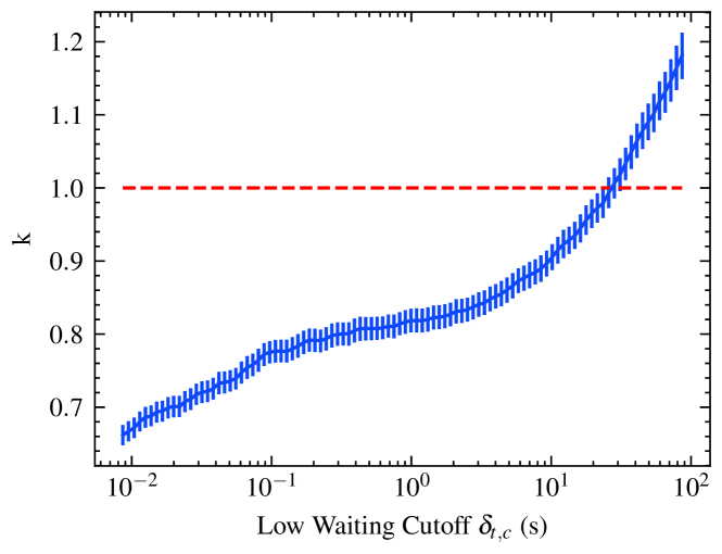
Oppermann et al. (2018) collected 17 bursts observed by Arecibo, Effelsberg, GBT, VLA, and Lovell. They derived with these 17 bursts. Oostrum et al. (2020) obtained . Their results are smaller than ours. This may be caused by the low waiting time cutoff. Cruces et al. (2021) found that when excluding the waiting time s, the shape parameter shifts from to . We carefully check the effect of waiting time cutoff and show the dependence of on in Figure 4. The solid blue line is the evolution of and the vertical solid blue lines are 1 errors. The shape parameter increases as increases. When , the shape parameter closes to 1, which means that the repeating behavior is due to a Poisson process. Cruces et al. (2021) also found that the waiting time with s is consistent with a Poisson process, which is similar to our results.
2.4 Linear repetition pattern
We use the FAST data to check the burst repetition pattern. We select the single-day observations with the number of detected bursts larger than 60 and show the cumulative distribution function of the burst time with blue scatters in each panel of Figure 5. The observation time is listed in the top of each panel. The x-axis is the decimal part of the MJD time. We find that the distribution can be fitted with a linear function
| (3) |
where is the burst time, is the slope, and is a constant. The best-fitting results with the dashed red lines are shown in each panel and the best-fitting parameters are also listed. The observation on 2019-09-07 is slightly different from other observations. There is an apparent temporal gap between early bursts occurring before MJD 58732.90 and late ones occurring after MJD 58732.90. In this observation, most bursts occurred after MJD 58732.90 and these bursts can be fitted with Equation (3). For all the observations listed in Figure 5, although the fitting results are different, they can be all fitted with equation 3. Tabor & Loeb (2020) proposed that the burst rate is constant per logarithmic time with the observation of GBT (Zhang et al., 2018). They found that the cumulative distribution function can be fitted with . Contrary, our results suggest that FAST strongly favors a linear pattern. Tabor & Loeb (2020) excluded the model that repeating FRB sources origin from pulsars (Beniamini et al., 2020). According to our results, this model is still feasible. The linear pattern may suggest a potentially short period. However, similar to Li et al. (2021a), we do not find any short period. The Lomb-Scargle method and epoch folding method are used to search between 10 milliseconds and 30 minutes. No significant period was found. The fluctuations of data points along the fitted lines in Figure 5 may suggest that the linear pattern is caused by the narrow waiting time distribution. Besides, the slopes in varied observations are different, which may suggest diverse waiting time distribution in different observations.
3 Discussion
3.1 Energy distribution in different epochs
An important conclusion of Li et al. (2021a) is the novel triple peaks structure in the KDE of energy and burst time (As shown in the panel (c) of their Figure 1). There is a clear energy gap between the high-energy bursts and low-energy bursts before MJD 58740. The temporal gap between early bursts and late bursts is also significant. Following the division of Li et al. (2021a), we regard the bursts occurring before MJD 58740 as early bursts and the bursts occurring after MJD 58740 as late bursts. The energy distributions of early bursts and late bursts are shown in Figure 6. Again, we only fit the bursts with energy erg. The best-fitting results are shown as green dot-dashed lines. The power-law index for the early bursts is (1 uncertainty), while that for the late bursts is (1 uncertainty), which is significantly different.
Some previous works support the power-law index (Wang & Yu, 2017; Law et al., 2017; Wang & Zhang, 2019), which is consistent with the result of early bursts. However, there are also some works suggest a steeper index (Gourdji et al., 2019), which is close to the result of late bursts. This difference may be caused by the following reasons. There may be different modes of burst emission operating in different epochs, so that the observed energy distribution may depend on the observing time. The two different modes may be related to different mechanisms or different emission sites. Li et al. (2021a) reported the triple peaks in the distribution of energy and burst time (as shown in panel (c) of their Figure 1). At the early epoch, the bursts with erg belong to the high-energy burst component. However, the high-energy peak is invisible in the late epoch. The bursts with erg in the late epoch are an extension of the low-energy peak. If the high-energy bursts and low-energy bursts originate from different mechanisms or different sites, which operate in different epochs, the variance of the energy distribution is naturally interpreted.
3.2 Waiting time for different energies
Li et al. (2021a) reported the triple peak structure in the panel (c) of their Figure 1. The bimodal structure in the energy distribution in the early phase (before MJD 58740) may suggest that they are produced by different physical processes. Therefore, we explore whether there are differences in their other properties, such as waiting time. If the low-energy bursts and high-energy bursts are produced by different processes, the waiting time should be calculated independently. We divide all bursts into three sub-samples: the low-energy bursts and high-energy bursts between MJD 58717 and 58740, and the late-phase bursts detected between MJD 58740 and 58776. The dividing line of burst time is consistent with the choice of Li et al. (2021a). We take the dividing line between the low-energy bursts and high-energy bursts as erg. The gap is about erg. For convenience, we take the separation line as erg. We also test other choices of the criteria and find that it does not affect on our result. For each sub-sample we calculate the waiting time independently and show the KDE of the waiting time in Figure 7. The KDE for these three sub-samples is slightly different. The medians of the low-energy bursts, high-energy bursts, and late-bursts are 78.19 s, 133.61 s, and 54.62 s, respectively. There is a small peak in the KDE density of the late-phase bursts, which is close to 0.1 s.
We also use the Weibull function to fit three sub-samples. Again, we ignore the waiting times with ms and day. We list the best-fitting results for three sub-samples in Table 1. The shape parameters are for the low-energy bursts, for the high-energy bursts and for the late-phase bursts. The posterior distributions of for the three sub-samples are shown in Figure 8. The parameters for the low-energy bursts, high-energy bursts, and late-phase bursts are shown as black line, red line, and blue line, respectively. The vertical dashed lines are the best-fitting results. The shape parameters for the low-energy and late-phase bursts are consistent with each other within 1 error, while the for the high-energy bursts is higher. The consistency of the low-energy bursts and late-phase bursts may suggest that they have the same origin, while the high-energy bursts may have a different origin. The difference between the late-phase bursts and high-energy bursts is significant, but the variance between the low-energy bursts and high-energy bursts is insignificant. This may be caused by the rough erg division line of low-energy bursts and high-energy bursts. The count distributions of low-energy and high-energy bursts are close to a log-normal distribution. They can be extended to include each other. Therefore, some FRBs may be misclassified. If we can make a robust classification, the difference in waiting time may be larger.
We derive the burst rates for the low-energy bursts and high-energy bursts are per day and per day, respectively. The burst rate of the low-energy bursts is higher than that of the high energy bursts. These two classes of bursts occurred in the same epoch. For the bursts occurring in late observation days, the burst rate is about per day, which is higher than that of low-energy bursts and high-energy bursts, but close to the sum of these two classes of bursts.
We also check the dependence of energy on waiting time. For X-ray flares of gamma-ray bursts, an anti-correlation is found between energy and waiting time (Yi et al., 2016). The scatter plot of energy and waiting time of the FAST FRB sample is shown in Figure 9. No significant dependence of energy on waiting time is found. We also check the dependence for three sub-samples and found no significant dependence.
3.3 Waiting time in different observational days
The FAST observations spanned two months in time, which covered most of the active window of FRB 121102. We can test the dependence of the burst behaviors on observing time. The observations lasted for roughly 1 hour each day. We regard the observations in each day as single samples and select some samples with the number of observed bursts greater than 5. Then, the Weibull function is applied to fit the waiting time distribution in these days. The best-fitting results against burst time are shown in Figure 10. The blue points are the shape parameters with errors, and the yellow points are the burst rates with errors. Interestingly, the value of is close to in some days, which indicates a rough Poisson distribution of the waiting time. Some observations have , which means that the waiting time prefers a specific value. If , it means a periodic behavior. In our calculation, the value of is not enough to support the periodic behavior. It only suggests that the waiting time has a narrow distribution in some days, which is consistent with the linear pattern. The best-fitting result varies for different samples. We do not find significant dependence on the observation time.
4 Conclusions
The energy and waiting time distributions of FRB 121102 provide a clue for understanding the physical origin of repeating FRBs. Li et al. (2021a) reported a large sample of bursts (1652), about 1200 of which are faint bursts with erg (the nominal threshold for separating low and high energy events). The detection of these faint bursts enables us to perform extensive statistical studies of the burst properties. Our conclusions can be summarized as follows.
-
1.
The energy distribution in the high-energy range can be fitted with a simple power-law function. The power-law index is , which is consistent with previous results (Wang & Yu, 2017; Law et al., 2017; Wang & Zhang, 2019; Cruces et al., 2021). This index is also similar to those of non-repeating FRBs (Cao et al., 2018; Lu & Piro, 2019) and magnetar X-ray bursts (Göǧüş et al., 2000; Cheng et al., 2020), which may suggest they share similar physical processes. However, the energy distribution deviates from this power-law function at low energies. The turning point is near erg, well above the 90% detection completeness threshold ( erg). Thus, this deviation is not caused by the incompleteness in the low-energy end. A different physical mechanism or different emission site for low-energy events may be required to explain this deviation.
-
2.
The Weibull function is used to fit the waiting times excluding events separated by ms and day. We derive and day-1. This result () suggests that the bursts of FRB 121102 tend to cluster in time. We also found that when we exclude the waiting time s, the burst behavior can be roughly described by a Poisson process.
-
3.
For bursts observed in a single day, a linear repetition pattern of burst time is found. We select the observational days when more than 60 bursts were detected. The cumulative distributions of the burst time are shown in Figure 5. These distributions can be fitted with .
-
4.
The distributions of high-energy early bursts and late bursts are different.The dividing line of early bursts and late bursts is MJD 58740. When the bursts with erg are considered, the power-law index is for early bursts and for late bursts. This difference may suggest that they have different physical origins.
-
5.
According to the bimodal structure of energy distribution reported by Li et al. (2021a), we divide the bursts into 3 classes: the low-energy bursts and high-energy bursts between MJD 58717 and 58740, and the late-phase bursts. The distributions of waiting time for these three classes are somewhat different. We also use the Weibull function to fit the waiting time distributions. The posterior probability distribution of the parameter for the high-energy bursts is slightly different from that of the low-energy and late-phase bursts. These differences may suggest that they have different physical origins or emission sites.
-
6.
There is no significant dependence of energy on waiting time. For three sub-samples, we also do not find any dependence between the two parameters.
Acknowledgements
We would like to thank the anonymous referee for helpful comments. This work was supported by the National Natural Science Foundation of China (grant No. 11988101, No. U1831207, No. 11833003, No. 11725313, No. 11690024, No. 12041303 and No. U2031117), the Fundamental Research Funds for the Central Universities (No. 0201-14380045), the National Key Research and Development Program of China (grant 2017YFA0402600); and the National SKA Program of China No. 2020SKA0120200, the Cultivation Project for FAST Scientific Payoff and Research Achievement of CAMS-CAS. PW acknowledges support by the Youth Innovation Promotion Association CAS (id. 2021055) and CAS Project for Young Scientists in Basic Reasearch (grant YSBR-006). This work made use of data from FAST, a Chinese national mega-science facility built and operated by the National Astronomical Observatories, Chinese Academy of Sciences.
References
- Ai et al. (2021) Ai, S., Gao, H., & Zhang, B. 2021, ApJ, 906, L5, doi: 10.3847/2041-8213/abcec9
- Aschwanden (2011) Aschwanden, M. J. 2011, Self-Organized Criticality in Astrophysics
- Bak et al. (1987) Bak, P., Tang, C., & Wiesenfeld, K. 1987, Phys. Rev. Lett., 59, 381, doi: 10.1103/PhysRevLett.59.381
- Beloborodov (2017) Beloborodov, A. M. 2017, ApJ, 843, L26, doi: 10.3847/2041-8213/aa78f3
- Beniamini et al. (2020) Beniamini, P., Wadiasingh, Z., & Metzger, B. D. 2020, MNRAS, 496, 3390, doi: 10.1093/mnras/staa1783
- Bochenek et al. (2020) Bochenek, C. D., Ravi, V., Belov, K. V., et al. 2020, Nature, 587, 59, doi: 10.1038/s41586-020-2872-x
- Caleb et al. (2019) Caleb, M., Stappers, B. W., Rajwade, K., & Flynn, C. 2019, MNRAS, 484, 5500, doi: 10.1093/mnras/stz386
- Caleb et al. (2020) Caleb, M., Stappers, B. W., Abbott, T. D., et al. 2020, MNRAS, 496, 4565, doi: 10.1093/mnras/staa1791
- Cao et al. (2018) Cao, X.-F., Yu, Y.-W., & Zhou, X. 2018, ApJ, 858, 89, doi: 10.3847/1538-4357/aabadd
- Chatterjee et al. (2017) Chatterjee, S., Law, C. J., Wharton, R. S., et al. 2017, Nature, 541, 58, doi: 10.1038/nature20797
- Cheng et al. (2020) Cheng, Y., Zhang, G. Q., & Wang, F. Y. 2020, MNRAS, 491, 1498, doi: 10.1093/mnras/stz3085
- CHIME/FRB Collaboration et al. (2019) CHIME/FRB Collaboration, Andersen, B. C., Bandura, K., et al. 2019, ApJ, 885, L24, doi: 10.3847/2041-8213/ab4a80
- CHIME/FRB Collaboration et al. (2020a) CHIME/FRB Collaboration, Andersen, B. C., Bandura, K. M., et al. 2020a, Nature, 587, 54, doi: 10.1038/s41586-020-2863-y
- CHIME/FRB Collaboration et al. (2020b) CHIME/FRB Collaboration, Amiri, M., Andersen, B. C., et al. 2020b, Nature, 582, 351, doi: 10.1038/s41586-020-2398-2
- Cordes & Chatterjee (2019) Cordes, J. M., & Chatterjee, S. 2019, ARA&A, 57, 417, doi: 10.1146/annurev-astro-091918-104501
- Cordes & Wasserman (2016) Cordes, J. M., & Wasserman, I. 2016, MNRAS, 457, 232, doi: 10.1093/mnras/stv2948
- Cruces et al. (2021) Cruces, M., Spitler, L. G., Scholz, P., et al. 2021, MNRAS, 500, 448, doi: 10.1093/mnras/staa3223
- Dai et al. (2016) Dai, Z. G., Wang, J. S., Wu, X. F., & Huang, Y. F. 2016, ApJ, 829, 27, doi: 10.3847/0004-637X/829/1/27
- Dai & Zhong (2020) Dai, Z. G., & Zhong, S. Q. 2020, ApJ, 895, L1, doi: 10.3847/2041-8213/ab8f2d
- Deng et al. (2021) Deng, C.-M., Zhong, S.-Q., & Dai, Z.-G. 2021, arXiv e-prints, arXiv:2102.06796. https://arxiv.org/abs/2102.06796
- Gajjar et al. (2018) Gajjar, V., Siemion, A. P. V., Price, D. C., et al. 2018, ApJ, 863, 2, doi: 10.3847/1538-4357/aad005
- Gourdji et al. (2019) Gourdji, K., Michilli, D., Spitler, L. G., et al. 2019, ApJ, 877, L19, doi: 10.3847/2041-8213/ab1f8a
- Göǧüş et al. (2000) Göǧüş, E., Woods, P. M., Kouveliotou, C., et al. 2000, ApJ, 532, L121, doi: 10.1086/312583
- Hardy et al. (2017) Hardy, L. K., Dhillon, V. S., Spitler, L. G., et al. 2017, MNRAS, 472, 2800, doi: 10.1093/mnras/stx2153
- Hessels et al. (2019) Hessels, J. W. T., Spitler, L. G., Seymour, A. D., et al. 2019, ApJ, 876, L23, doi: 10.3847/2041-8213/ab13ae
- Hilmarsson et al. (2021) Hilmarsson, G. H., Michilli, D., Spitler, L. G., et al. 2021, ApJ, 908, L10, doi: 10.3847/2041-8213/abdec0
- Ioka & Zhang (2020) Ioka, K., & Zhang, B. 2020, ApJ, 893, L26, doi: 10.3847/2041-8213/ab83fb
- Katz (2019) Katz, J. I. 2019, MNRAS, 487, 491, doi: 10.1093/mnras/stz1250
- Kuerban et al. (2021) Kuerban, A., Huang, Y.-F., Geng, J.-J., et al. 2021, arXiv e-prints, arXiv:2102.04264. https://arxiv.org/abs/2102.04264
- Law et al. (2017) Law, C. J., Abruzzo, M. W., Bassa, C. G., et al. 2017, ApJ, 850, 76, doi: 10.3847/1538-4357/aa9700
- Levin et al. (2020) Levin, Y., Beloborodov, A. M., & Bransgrove, A. 2020, ApJ, 895, L30, doi: 10.3847/2041-8213/ab8c4c
- Li et al. (2018) Li, D., Wang, P., Qian, L., et al. 2018, IEEE Microwave Magazine, 19, 112, doi: 10.1109/MMM.2018.2802178
- Li et al. (2021a) Li, D., Wang, P., Zhu, W. W., et al. 2021a, arXiv e-prints, arXiv:2107.08205. https://arxiv.org/abs/2107.08205
- Li et al. (2021b) Li, Q.-C., Yang, Y.-P., Wang, F. Y., et al. 2021b, arXiv e-prints, arXiv:2108.00350. https://arxiv.org/abs/2108.00350
- Li et al. (2015) Li, Y.-P., Yuan, F., Yuan, Q., et al. 2015, ApJ, 810, 19, doi: 10.1088/0004-637X/810/1/19
- Lu & Piro (2019) Lu, W., & Piro, A. L. 2019, ApJ, 883, 40, doi: 10.3847/1538-4357/ab3796
- Luo et al. (2018) Luo, R., Lee, K., Lorimer, D. R., & Zhang, B. 2018, MNRAS, 481, 2320, doi: 10.1093/mnras/sty2364
- Luo et al. (2020) Luo, R., Men, Y., Lee, K., et al. 2020, MNRAS, 494, 665, doi: 10.1093/mnras/staa704
- Lyu et al. (2021) Lyu, F., Meng, Y.-Z., Tang, Z.-F., et al. 2021, Frontiers of Physics, 16, 24503, doi: 10.1007/s11467-020-1039-4
- Lyutikov et al. (2020) Lyutikov, M., Barkov, M. V., & Giannios, D. 2020, ApJ, 893, L39, doi: 10.3847/2041-8213/ab87a4
- Marcote et al. (2017) Marcote, B., Paragi, Z., Hessels, J. W. T., et al. 2017, ApJ, 834, L8, doi: 10.3847/2041-8213/834/2/L8
- Metzger et al. (2019) Metzger, B. D., Margalit, B., & Sironi, L. 2019, MNRAS, 485, 4091, doi: 10.1093/mnras/stz700
- Michilli et al. (2018) Michilli, D., Seymour, A., Hessels, J. W. T., et al. 2018, Nature, 553, 182, doi: 10.1038/nature25149
- Murase et al. (2016) Murase, K., Kashiyama, K., & Mészáros, P. 2016, MNRAS, 461, 1498, doi: 10.1093/mnras/stw1328
- Nan et al. (2011) Nan, R., Li, D., Jin, C., et al. 2011, International Journal of Modern Physics D, 20, 989, doi: 10.1142/S0218271811019335
- Oostrum et al. (2020) Oostrum, L. C., Maan, Y., van Leeuwen, J., et al. 2020, A&A, 635, A61, doi: 10.1051/0004-6361/201937422
- Oppermann et al. (2018) Oppermann, N., Yu, H.-R., & Pen, U.-L. 2018, MNRAS, 475, 5109, doi: 10.1093/mnras/sty004
- Palaniswamy et al. (2018) Palaniswamy, D., Li, Y., & Zhang, B. 2018, ApJ, 854, L12, doi: 10.3847/2041-8213/aaaa63
- Petroff et al. (2019) Petroff, E., Hessels, J. W. T., & Lorimer, D. R. 2019, A&A Rev., 27, 4, doi: 10.1007/s00159-019-0116-6
- Planck Collaboration & et al. (2016) Planck Collaboration, & et al. 2016, A&A, 594, A13, doi: 10.1051/0004-6361/201525830
- Popov & Stappers (2007) Popov, M. V., & Stappers, B. 2007, A&A, 470, 1003, doi: 10.1051/0004-6361:20066589
- Prieskorn & Kaaret (2012) Prieskorn, Z., & Kaaret, P. 2012, ApJ, 755, 1, doi: 10.1088/0004-637X/755/1/1
- Rajwade et al. (2020) Rajwade, K. M., Mickaliger, M. B., Stappers, B. W., et al. 2020, MNRAS, 495, 3551, doi: 10.1093/mnras/staa1237
- Ravi (2019) Ravi, V. 2019, Nature Astronomy, 405, doi: 10.1038/s41550-019-0831-y
- Scholz et al. (2016) Scholz, P., Spitler, L. G., Hessels, J. W. T., et al. 2016, ApJ, 833, 177, doi: 10.3847/1538-4357/833/2/177
- Scholz et al. (2017) Scholz, P., Bogdanov, S., Hessels, J. W. T., et al. 2017, ApJ, 846, 80, doi: 10.3847/1538-4357/aa8456
- Spitler et al. (2014) Spitler, L. G., Cordes, J. M., Hessels, J. W. T., et al. 2014, ApJ, 790, 101, doi: 10.1088/0004-637X/790/2/101
- Spitler et al. (2016) Spitler, L. G., Scholz, P., Hessels, J. W. T., et al. 2016, Nature, 531, 202, doi: 10.1038/nature17168
- Spitler et al. (2018) Spitler, L. G., Herrmann, W., Bower, G. C., et al. 2018, ApJ, 863, 150, doi: 10.3847/1538-4357/aad332
- Tabor & Loeb (2020) Tabor, E., & Loeb, A. 2020, ApJ, 902, L17, doi: 10.3847/2041-8213/abba79
- Tendulkar et al. (2017) Tendulkar, S. P., Bassa, C. G., Cordes, J. M., et al. 2017, ApJ, 834, L7, doi: 10.3847/2041-8213/834/2/L7
- Wada et al. (2021) Wada, T., Ioka, K., & Zhang, B. 2021, arXiv e-prints, arXiv:2105.14480. https://arxiv.org/abs/2105.14480
- Wadiasingh & Timokhin (2019) Wadiasingh, Z., & Timokhin, A. 2019, ApJ, 879, 4, doi: 10.3847/1538-4357/ab2240
- Wang & Dai (2013) Wang, F. Y., & Dai, Z. G. 2013, Nature Physics, 9, 465, doi: 10.1038/nphys2670
- Wang et al. (2015) Wang, F. Y., Dai, Z. G., Yi, S. X., & Xi, S. Q. 2015, ApJS, 216, 8, doi: 10.1088/0067-0049/216/1/8
- Wang & Yu (2017) Wang, F. Y., & Yu, H. 2017, J. Cosmology Astropart. Phys, 03, 023, doi: 10.1088/1475-7516/2017/03/023
- Wang & Zhang (2019) Wang, F. Y., & Zhang, G. Q. 2019, ApJ, 882, 108, doi: 10.3847/1538-4357/ab35dc
- Xiao et al. (2021) Xiao, D., Wang, F., & Dai, Z. 2021, arXiv e-prints, arXiv:2101.04907. https://arxiv.org/abs/2101.04907
- Yang & Zou (2020) Yang, H., & Zou, Y.-C. 2020, ApJ, 893, L31, doi: 10.3847/2041-8213/ab800f
- Yang et al. (2019) Yang, S., Yan, D., Dai, B., et al. 2019, MNRAS, 489, 2685, doi: 10.1093/mnras/stz2302
- Yang et al. (2021) Yang, Y.-H., Zhang, B.-B., Lin, L., et al. 2021, ApJ, 906, L12, doi: 10.3847/2041-8213/abd02a
- Yang & Zhang (2021) Yang, Y.-P., & Zhang, B. 2021, arXiv e-prints, arXiv:2104.01925. https://arxiv.org/abs/2104.01925
- Yi et al. (2016) Yi, S.-X., Xi, S.-Q., Yu, H., et al. 2016, ApJS, 224, 20, doi: 10.3847/0067-0049/224/2/20
- Zanazzi & Lai (2020) Zanazzi, J. J., & Lai, D. 2020, ApJ, 892, L15, doi: 10.3847/2041-8213/ab7cdd
- Zhang (2018) Zhang, B. 2018, ApJ, 867, L21, doi: 10.3847/2041-8213/aae8e3
- Zhang (2020) —. 2020, Nature, 587, 45, doi: 10.1038/s41586-020-2828-1
- Zhang et al. (2019) Zhang, G. Q., Wang, F. Y., & Dai, Z. G. 2019, arXiv e-prints, arXiv:1903.11895. https://arxiv.org/abs/1903.11895
- Zhang et al. (2021) Zhang, R. C., Zhang, B., Li, Y., & Lorimer, D. R. 2021, MNRAS, 501, 157, doi: 10.1093/mnras/staa3537
- Zhang et al. (2018) Zhang, Y. G., Gajjar, V., Foster, G., et al. 2018, ApJ, 866, 149, doi: 10.3847/1538-4357/aadf31
| Data set | (day-1) | |
|---|---|---|
| All bursts of Li et al. (2021a) | ||
| low-energy bursts | ||
| high-energy bursts | ||
| late-phase bursts | ||
| Oppermann et al. (2018) | ||
| Oostrum et al. (2020) | ||
| Cruces et al. (2021) |