Energetic Variational Neural Network Discretizations of Gradient Flows
Abstract
We present a structure-preserving Eulerian algorithm for solving -gradient flows and a structure-preserving Lagrangian algorithm for solving generalized diffusions. Both algorithms employ neural networks as tools for spatial discretization. Unlike most existing methods that construct numerical discretizations based on the strong or weak form of the underlying PDE, the proposed schemes are constructed based on the energy-dissipation law directly. This guarantees the monotonic decay of the system’s free energy, which avoids unphysical states of solutions and is crucial for the long-term stability of numerical computations. To address challenges arising from nonlinear neural network discretization, we perform temporal discretizations on these variational systems before spatial discretizations. This approach is computationally memory-efficient when implementing neural network-based algorithms. The proposed neural network-based schemes are mesh-free, allowing us to solve gradient flows in high dimensions. Various numerical experiments are presented to demonstrate the accuracy and energy stability of the proposed numerical schemes.
1 Introduction
Evolution equations with variational structures, often termed as gradient flows, have a wide range of applications in physics, material science, biology, and machine learning [14, 60, 78]. These systems not only possess but also are determined by an energy-dissipation law, which consists of an energy of state variables that describes the energetic coupling and competition, and a dissipative mechanism that drives the system to an equilibrium.
More precisely, beginning with a prescribed energy-dissipation law
| (1) |
where is the sum of the Helmholtz free energy and the kinetic energy , and is the rate of energy dissipation, one could derive the dynamics, the corresponding partial differential equation (PDE), of the system by combining the Least Action Principle (LAP) and the Maximum Dissipation Principle (MDP). The LAP states that the equation of motion of a Hamiltonian system can be derived from the variation of the action functional with respect to state variable . This gives rise to a unique procedure to derive the “conservative force” in the system. The MDP, on the other hand, derives the “dissipative force” by taking the variation of the dissipation potential , which equals to in the linear response regime (near equilibrium), with respect to . In turn, the force balance condition leads to the PDE of the system:
| (2) |
This procedure is known as the energetic variational approach (EnVarA) [24, 48, 74], developed based on the celebrated work of Onsager [57, 58] and Rayleigh [63] in non-equilibrium thermodynamics. During the past decades, the framework of EnVarA has shown to be a powerful tool for developing thermodynamically consistent models for various complex fluid systems, including two-phase flows [80, 81, 83], liquid crystals [48], ionic solutions [22], and reactive fluids [75, 76]. In a certain sense, the energy-dissipation law (1), which comes from the first and second law of thermodynamics [23], provides a more intrinsic description of the underlying physics than the derived PDE (2), in particularly for systems that possess multiple structures and involve multiscale and multiphysics coupling.
From a numerical standpoint, the energy-dissipation law (1) also serves as a valuable guideline for developing structure-preserving numerical schemes for these variational systems, as many straightforward PDE-based discretizations may fail to preserve the continuous variational structures, as well as the physical constraints, such as the conservation of mass or momentum, the positivity of mass density, and the dissipation of the energy. As a recent development in this field [50], the authors proposed a numerical framework, called a discrete energetic variational approach, to address these challenges. Similar methods are also used in [72, 82]. The key idea of this approach is to construct numerical discretizations directly based on the continuous energy-dissipation laws without using the underlying PDE (see Section 3.1 for details). The approach has advantages in preserving a discrete counterpart of the continuous energy dissipation law, which is crucial for avoiding unphysical solutions and the long-term stability of numerical computations. Within the framework of the discrete energetic variational approach, Eulerian [55], Lagrangian [50, 51], and particle methods [73] have been developed for various problems.
However, tackling high-dimensional variational problems remains a challenge. Traditional numerical discretization, such as finite difference, finite element, and finite volume methods, suffer from the well-known curse of dimensionality (CoD) [27]. Namely, the computational complexity of the numerical algorithm increases exponentially as a function of the dimensionality of the problem [4, 27]. Although particle methods hold promise for addressing high-dimensional problems, standard particle methods often lack accuracy and are not suitable for problems involving derivatives.
During the recent years, neural networks (NNs) have demonstrated remarkable success across a wide spectrum of scientific disciplines [12, 31, 41, 43, 47]. Leveraging the potent expressive power of neural network [3, 10, 20], particularly deep neural network (DNN) architectures, there exists a growing interest in developing neural network-based algorithms for PDEs, especially for those in high dimensions [13, 21, 37, 38, 42, 62, 68, 70, 77]. Examples include physics-informed neural network (PINN) [62], deep Ritz method (DRM) [21], deep Galerkin method (DGM) [68], variational PINN [37], and weak adversarial network (WAN) [84] to name a few. A key component of these aforementioned approaches is to represent solutions of PDEs via NNs. All of these approaches determine the optimal parameters of the NN by minimizing a loss function, which is often derived from either the strong or weak form of the PDE (see section 2.1 for more details). By employing NN approximations, the approximate solution belongs to a space of nonlinear functions, which may lead to a robust estimation by sparser representation and cheaper computation [37].
The goal of this paper is to combine neural network-based spatial discretization with the framework of the discrete energetic variational approach [50], to develop efficient and robust numerical schemes, termed as energetic variational neural network (EVNN) methods. To clarify the idea, we consider the following two types of gradient flows modeled by EnVarA:
-
•
-gradient flow that satisfies an energy-dissipation law
(3) -
•
Generalized diffusion that satisfies an energy-dissipation law
(4) where satisfies , known as the mass conservation.
Derivation of the underlying PDEs for these types of systems is described in Sections 2.1.1 and 2.1.2 of the paper.
Our primary aim is to develop structure-preserving Eulerian algorithms to solve -gradient flows and structure-preserving Lagrangian algorithms to solve generalized diffusions based on their energy-dissipation law by utilizing neural networks as a new tool of spatial discretization. To overcome difficulties arising from neural network discretization, we develop a discretization approach that performs temporal discretizations before spatial discretizations. This approach leads to a computer-memory-efficient implementation of neural network-based algorithms. Since neural networks are advantageous due to their ability to serve as parametric approximations for unknown functions even in high dimensions, the proposed neural-network-based algorithms are capable of solving gradient flows in high-dimension, such as these appear in machine learning [19, 32, 69, 73].
The rest of the paper is organized as follows. Section 2 reviews the EnVarA and some existing neural network-based numerical approaches for solving PDEs. Section 3 of the paper is devoted to the development of the proposed EVNN schemes for -gradient flows and generalized diffusions. Various numerical experiments are presented in Section 4 to demonstrate the accuracy and energy stability of the proposed numerical methods. Conclusions are drawn in Section 5.
2 Preliminary
2.1 Energetic Variational Approach
In this subsection, we provide a detailed derivation of underlying PDEs for -gradient flows and generalized diffusions by the general framework of EnVarA. We refer interested readers to [24, 74] for a more comprehensive review of the EnVarA. In both systems, the kinetic energy .
2.1.1 -gradient flow
-gradient flows are those systems satisfying the energy-dissipation law:
| (5) |
where is the state variable, is the Helmholtz free energy, and is the dissipation rate. One can also view as the generalized coordinates of the system [14]. By treating as , the variational procedure (2) leads to the following -gradient flow equation:
Many problems in soft matter physics, material science, and machine learning can be modeled as -gradient flows. Examples include Allen–Cahn equation [15], Oseen–Frank and Landau–de Gennes models of liquid crystals [11, 45], phase field crystal models of quasicrystal [34, 44], and generalized Ohta–Kawasaki model of diblock and triblock copolymers [56]. For example, by taking
which is the classical Ginzburg–Landau free energy, and letting , one gets the Allen–Cahn equation
2.1.2 Generalized diffusion
Generalized diffusion describes the space-time evolution of a conserved quantity . Due to the physics law of mass conservation, satisfies the kinematics
| (6) |
where is an averaged velocity in the system.
To derive the generalized diffusion equation by the EnVarA, one should introduce a Lagrangian description of the system. Given a velocity field , one can define a flow map through
where is the Lagrangian coordinates and is the Eulerian coordinates. Here is the initial configuration of the system, and is the configuration of the system at time . For a fixed , describes the trajectory of a particle (or a material point) labeled by ; while for a fixed , is a diffeomorphism from to (See Fig. 1 for the illustration.) The existence of the flow map requires a certain regularity of , for instance, being Lipschitz in .

In a Lagrangian picture, the evolution of the density function is determined by the evolution of the through the kinematics relation (6) (written in the Lagrangian frame of reference). More precisely, one can define the deformation tensor associated with the flow map by
| (7) |
Without ambiguity, we do not distinguish and in the rest of the paper. Let be the initial density, then the mass conservation indicates that
| (8) |
in the Lagrangian frame of reference. This is equivalent to in the Eulerian frame.
Within (8), one can rewrite the energy-dissipation law (4) in terms of the flow map and its velocity in the reference domain . A typical form of the free energy is given by
| (9) |
where is a potential field, and is a symmetric non-local interaction kernel. In Lagrangian coordinates, the free energy (9) and the dissipation in (4) become
and
By a direct computation, the force balance equation (2) can be written as (see [24] for a detailed computation)
| (10) |
In Eulerian coordinates, combining (10) with the kinematics equation (6), one obtains a generalized diffusion equation
| (11) |
where is known as the mobility in physics. Many PDEs in a wide range of applications, including the porous medium equations (PME) [71], nonlinear Fokker–Planck equations [35], Cahn–Hilliard equations [50], Keller–Segel equations [36], and Poisson–Nernst–Planck (PNP) equations [22], can be obtained by choosing and differently.
The velocity equation (10) can be viewed as the equation of the flow map in Lagrangian coordinates, i.e.,
| (12) |
where . The flow map equation (12) is a highly nonlinear equation of that involves both and . It is rather unclear how to introduce a suitable spatial discretization to Eq. (12) by looking at the equation. However, a generalized diffusion can be viewed as an -gradient flow of the flow map in the space of diffeomorphism. This perspective gives rise to a natural discretization of generalized diffusions [50].
Remark 2.1.
In the case that , a generalized diffusion can be viewed as a Wasserstein gradient flows in the space of all probability densities having finite second moments [35]. Formally, the Wasserstein gradient flow can be defined as a continuous time limit () from a semi-discrete JKO scheme,
| (13) |
where and is the Wasserstein distance between and . The Wasserstein gradient flow is an Eulerian description of these systems [6]. Other choices of dissipation can define other metrics in the space of probability measures [1, 46].
2.2 Neural-network-based numerical schemes for PDEs
In this subsection, we briefly review some existing neural network-based algorithms for solving PDEs. We refer interested readers to [18, 52] for detailed reviews.
Considering a PDE subject to a certain boundary condition
| (14) |
and assuming the solution can be approximated by a neural network , where is the set of parameters in the neural network, the Physics-Informed Neural Network (PINN) [62] and similar methods [13, 68, 77] find the optimal parameter by minimizing a loss function defined as:
| (15) |
Here and are sets of samples in and respectively, which can be drawn uniformly or by following some prescribed distributions. The parameter is used to weight the sum in the loss function. Minimizers of the loss function (15) can be obtained by using some optimization methods, such as AdaGrad and Adam. Of course, the objective function of this minimization problem in general is not convex even when the initial problem is. Obtaining the global minimum of (15) is highly non-trivial.
In contrast to the PINN, which is based on the strong form of a PDE, the deep Ritz method (DRM) [21] is designed for solving PDEs using their variational formulations. If Eq. (14) is an Euler-Lagrangian equation of some energy functional
| (16) |
then the loss function can be defined directly by
| (17) |
The last term in (16) is a penalty term for the boundary condition. The original Dirichlet boundary condition can be recovered with . Again, the samples and can be uniformly sampled from and or sampled following some other prescribed distributions, respectively. Additionally, both the variational PINN [37] and the WAN [84] utilized the Galerkin formulation to solve PDEs. The variational PINN [37], stems from the Petrov–Galerkin method, represents the solution via a DNN, and keeps test functions belonging to linear function spaces. The WAN employs the primal and adversarial networks to parameterize the weak solution and test functions respectively [84].
The neural network-based algorithms mentioned above focus on elliptic equations. For an evolution equation of the form:
| (18) |
with a suitable boundary condition, the predominant approach is to treat the time variable as an additional dimension, and the PINN type techniques can be applied. However, these approaches are often expensive and may fail to capture the dynamics of these systems. Unlike spatial variables, there exists an inherent order in time, where the solution at time is determined by the solutions in . It is difficult to generate samples in time to maintain this causality. Very recently, new efforts have been made in using NNs to solve evolution PDEs [8, 16]. The idea of these approaches is to use NNs with time-dependent parameters to represent the solutions. For instance, Neural Galerkin method, proposed in [8], parameterizes the solution as with being the NN parameters, and defines a loss function in terms of and through a residual function, i.e.,
| (19) |
where is a suitable measure which might depend on . By taking variation of with respect to , the neural Galerkin method arrives at an ODE of :
| (20) |
where and The ODE (20) can be solved by standard explicit or implicit time-marching schemes.
It’s important to note that, with the exception of DRM, all existing neural-network-based methods are developed based on either the strong or weak forms of PDEs. While DRM utilizes the free energy functional, it is only suitable for solving static problems, i.e., finding the equilibrium of the system. Additionally, most of these existing approaches are Eulerian methods. For certain types of PDEs, like generalized diffusions, these methods may fail to preserve physical constraints, such as positivity and the conservation of mass of a probability function.
3 Energetic Variational Neural Network
In this section, we present the structure-preserving EVNN discretization for solving both -gradient flows and generalized diffusions, As mentioned earlier, the goal is to construct a neural-network discretization based on the energy-dissipation law, without working on the underlying PDE. One can view our method as a generalization of the DRM to evolution equations.
3.1 EVNN scheme for -gradient flow
Before we discuss the neural network discretization, we first briefly review the discrete energetic variational approach proposed in [50]. Given a continuous energy-dissipation law (1), the discrete energetic variational approach first constructs a finite-dimensional approximation to a continuous energy-dissipation law by introducing a spatial discretization of the state variable , denoted by , where is the parameter to be determined. By replacing by , one obtain a semi-discrete energy-dissipation law (here we assume in the continuous model for simplicity) in terms of :
| (21) |
where , and For example, in Galerkin methods, one can let be with being the set of basis functions. Then is a vector given by .
By employing the energetic variational approach in the semi-discrete level (21), one can obtain an ODE system of . Particularly, in the linear response regime, is a quadratic function of . The ODE system of can then be written as
| (22) |
where
| (23) |
The ODE (22) is the same as the ODE (20) in the neural Galerkin method [8] for gradient flows, although the derivation is different.
Since (22) is a finite-dimensional gradient flow, one can then construct a minimizing movement scheme for [25]: finding such that
| (24) |
Here is the admissible set of inherited from the admissible set of , denoted by , and is a constant matrix. A typical choice of . An advantage of this scheme is that
| (25) |
if is positive definite, which guarantees the energy stability for the discrete free energy . Moreover, by choosing a proper optimization method, we can assure that stays in the admissible set .
Although neural networks can be used to construct , it might be expensive to compute in . Moreover, is not a sparse matrix and requires a lot of computer memory to store when a deep neural network is used.
To overcome these difficulties, we propose an alternative approach by introducing temporal discretization before spatial discretization. Let be the time step size. For the -gradient flow (5), given , which represents the numerical solution at , one can obtain by solving the following optimization problem: finding in some admissible set such that
| (26) |
Let be a finite-dimensional approximation to with being the parameter of the spatial discretization (e.g., weights of linear combination in a Galerkin approximation) yet to be determined, then the minimizing movement scheme (26) can be written in terms of : finding such that
| (27) |
Here is the value of at time . , and .
Remark 3.1.
The connection between the minimizing movement scheme (27) derived by a temporal-then-spatial approach, and the minimizing movement scheme (24) derived by a spatial-then-temporal approach, can be shown with a direct calculation. Indeed, according to the first-order necessary condition for optimality, an optimal solution to the minimization problem (27) satisfies
| (28) | ||||
for some , where the second equality follows the mean value theorem. In the case of Galerkin methods, as is independent on , is a solution to an implicit Euler scheme for the ODE (22) in which is treated explicitly.
By choosing a certain neural network to approximate , denoted by ( is used to denote all parameters in the neural network), we can summarize the EVNN scheme for solving a -gradient flow in Alg. 1.
For a given initial condition , compute by solving
| (29) |
At each step, update by solving the optimization problem
| (30) |
We have as a numerical solution at time .
It can be noticed that both Eq. (29) and Eq. (30) involve integration in the computational domain . This integration is often computed by using a grid-based numerical quadrature or Monte–Carlo/Quasi–Monte–Carlo algorithms [65]. It is worth mentioning that due to the non-convex nature of the optimization problem and the error in estimating the integration, it might be difficult to find an optimal at each step. But since we start the optimization procedure with , we’ll always be able to get a that lowers the discrete free energy at least on the training set. In practice, the optimization problem can be solved by either deterministic optimization algorithms, such as L-BFGS and gradient descent with Barzilai–Borwein step-size, or stochastic gradient descent algorithms, such as AdaGrad and Adam.
Remark 3.2.
It is straightforward to incorporate other variational high-order temporal discretizations to solve the -gradient flows. For example, a second-order accurate BDF2 scheme can be reformulated as an optimization problem
| (31) | ||||
A modified Crank–Nicolson time-marching scheme can be reformulated as
| (32) | ||||
Here we assume that is a constant for simplicity.
3.2 Lagrangian EVNN scheme for generalized diffusions
In this subsection, we show how to formulate an EVNN scheme in the Lagrangian frame of reference for generalized diffusions.
As discussed previously, a generalized diffusion can be viewed as an -gradient flow of the flow map in the space of diffeomorphisms. Hence, the EVNN scheme for the generalized diffusion can be formulated in terms of a minimizing movement scheme of the flow map given by
| (33) |
where is a numerical approximation of the flow map at , is the initial density. is the free energy for the generalized diffusion defined in Eq. (9), and
One can parameterize by a suitable neural network. The remaining procedure is almost the same as that of the last subsection. However, it is often difficult to solve this optimization problem directly, and one might need to build a large neural network to approximate when is large.
To overcome this difficulty, we proposed an alternative approach, Instead of seeking an optimal map between and , we seek an optimal between and . More precisely. we assume that
Given , one can compute by solving the following optimization problem
| (34) |
The corresponding can then be computed through . An advantage of this approach is that we only need a small size of neural network to approximate at each time step when is small.
Remark 3.3.
The scheme (34) can be viewed as a Lagrangian realization of the JKO scheme (13) for the Wasserstein gradient flow, although it is developed based on the -gradient flow structure in the space of diffeomorphism. According to the Benamou–Brenier formulation [5], the Wasserstein distance between two probability densities and can be computed by solving the optimization problem
| (35) |
where the admissible set of is given by
| (36) |
Hence, one can solve the JKO scheme by solving
| (37) | ||||
and letting . In Lagrangian coordinates, (37) is equivalent to
| (38) |
where and . By taking variation of (38) with respect to , one can show that the optimal condition is for , which indicates that if . Hence, if is the optimal solution of (34), then is the optimal solution of (38).
Remark 3.4.
If , we can formulate the optimization problem (34) as
| (39) |
by treating explicit. A subtle fact is that since we always start with an identity map.
The numerical algorithm for solving the generalized diffusion is summarized in Alg. 2.
-
•
Given and the densities at and .
- •
-
•
After obtaining , updates and by
(40)
The next question is how to accurately evaluate the numerical integration in (34). Let , for the general free energy (9), one way to evaluate the integrations in Eq. (34) is using
| (41) | ||||
where is the volume of the Voronoi cells associated with the set of points , stands for . Here the numerical integration is computed through a piece-wisely constant reconstruction of based on its values at . However, it is not straightforward to compute , particularly for high dimensional cases. In the current study, we assume that the initial samples are drawn from , one can roughly assume that follows the distribution , then according to the Monte–Carlo approach, the numerical integration can be evaluated as
| (42) | ||||
where The proposed numerical method can be further improved if one can evaluate the integration more accurately, i.e., have an efficient way to estimate . Alternatively, as an advantage of the neural network-based algorithm, we can get , which enables us to estimate by resampling. More precisely, assume is a distribution that is easy to sample
| (43) | ||||
where , . We will explore this resampling approach in future work.
The remaining question is how to parameterize a diffeomorphism using neural networks. This is discussed in detail in the next subsection.
3.3 Neural network architectures
In principle, the proposed numerical framework is independent of the choice of neural network architectures. However, different neural network architectures may lead to different numerical performances, arising from a balance of approximation (representation power), optimization, and generalization. In this subsection, we briefly discuss several neural network architectures that we use in the numerical experiments.
3.3.1 Neural network architectures for Eulerian methods
For Eulerian methods, one can construct a neural network to approximate the unknown function . Shallow neural networks (two-layer neural networks) approximate by functions of the form
| (44) |
where is a fixed nonlinear activation function, is the number of hidden nodes (neurons), and are the NN parameters to be identified. Typical choices of activation functions include the ReLU , the sigmoid and the hyperbolic tangent function .A DNN can be viewed as a network composed of many hidden layers. More precisely, a DNN with hidden layers represents a function by [67]
| (45) |
where is a linear map from to , is a nonlinear map from to , and . The nonlinear map takes the form
| (46) |
where , and is a nonlinear activation function that acts component-wisely on vector-valued inputs.
Another widely used class of DNN model is residual neural network (ResNet). A typical -block ResNet approximates an unknown function by
| (47) |
where is a linear map from and is a nonlinear map defined through
| (48) |
Here is the number of fully connected layer in -the block, is the same nonlinear map defined in (46) with , , , and is an element-wise activation function. The model parameters are . The original ResNet [29] takes as a nonlinear activation function such as ReLU. Later studies indicate that one can also take as the identity function [18, 30]. Then at an infinite length, i.e., , (48) corresponds to the ODE
| (49) |
Compared with fully connected deep neural network models which may suffer from numerical instabilities in the form of exploding or vanishing gradients [19, 28, 40], very deep ResNet can be constructed to avoid these issues.
Given that the proposed numerical scheme employs neural networks with time-dependent parameters to approximate the solution of a gradient flow, there is no need to employ a deep neural network. In all numerical experiments for -gradient flows, we utilize ResNet with only a few blocks. The detailed neural network settings for each numerical experiment will be described in the next section. We’ll compare the numerical performance of different neural network architectures in future work.
3.3.2 Neural network architectures for Lagrangian methods
The proposed Lagrangian method seeks for a neural network to approximate a diffeomorphism from to . This task involves two main challenges: one is ensuring that the map is a diffeomorphism, and the other is efficiently and robustly computing the deformation tensor and its determinant . Fortunately, various neural network architectures have been proposed to approximate a transport map. Examples include planar flows [64], auto-regressive flows [39], continuous-time diffusive flow [69], neural spline flow [17], and convex potential flow [32].
One way to construct a neural network for approximating a flow map is to use a planar flow. A -layer planar flow is defined by , where is given by
| (50) |
Here, , , and is a smooth, element-wise, non-linear activation function such as . Direct computation shows that
| (51) |
Clearly, is a diffeomorphism if for . The determinant of the transport map can be computed as . and we have .
One limitation of planar flow is its potential lack of expressive power. Another commonly employed neural network architecture for approximating a flow map is the convex potential flow [32], which defines a diffeomorphism via the gradient of a strictly convex function that is parameterized by an Input Convex Neural Network (ICNN) [2]. A fully connected, layer ICNN can be written as
| (52) |
where , , are the parameters to be determined, and is the nonlinear activation function. As proved in [2], if all entries are non-negative, and all are convex and non-decreasing, then is a convex function with respect to . Hence provides a parametric approximation to a flow map. In the current study, we adopt the concept of the convex potential flow to develop the Lagrangian EVNN method. We’ll explore other types of neural network architectures in future work.
Remark 3.5.
It is worth mentioning that the gradient of a convex function only defines a subspace of diffeomorphism, and it is unclear whether the optimal solution of (34) belongs to this subspace.
4 Numerical Experiments
In this section, we test the proposed EVNN methods for various -gradient flows and generalized diffusions. To evaluate the accuracy of different methods, we define the -error
and the relative -error
between the NN solution and the corresponding reference solution on a set of test samples . The reference solution is either an analytic solution or a numerical solution obtained by a traditional numerical method. In some numerical examples, we also plot point-wise absolute errors at the grid points.
4.1 Poisson equations
Although the proposed method is designed for evolutionary equations, it can also be used to compute equilibrium solutions for elliptic problems. In this subsection, we compare the performance of the EVNN method with two classical neural network-based algorithms, PINN and DRM, in the context of solving Poisson equations.
We first consider a 2D Poisson equation with a Dirichlet boundary condition
| (53) |
Since EVNN is developed for evolution equations, we solve the following gradient flow
| (54) |
to get a solution of the Poisson equation (53). Here, is the surface energy that enforces the Dirichlet boundary condition. The corresponding gradient flow equation is given by
| (55) |
subject to a Robin boundary condition , where is the outer normal of . One can recover the original Dirichlet boundary condition by letting . Such a penalty approach is also used in PINN and DRM, and we take in all numerical experiments below.
We consider the following two cases:
-
•
Case 1: , and . The exact solution is .
-
•
Case 2: , and . The exact solution is .
We employ a 1-block ResNet with 20 hidden nodes and one hidden layer for all cases. The total number of parameters is 501. We apply Xavier Initialization [26] to initialize the weights of neural networks in all cases. To evaluate the integration in all methods, we generate samples in using a Latin hypercube sampling (LHS) and samples on each boundary of using a 1D uniform sampling for case 1. For case 2, we generate samples in using LHS, but only use the samples satisfies as training samples. Additionally, we generate 200 training samples on the boundary, with being generated by a uniform distribution on . For PINN and DRM, we use Adam to minimize the loss function and use a different set of samples at each iteration. For EVNN, we use a different set of samples at each time step and employ an L-BFGS to solve the optimization problem (30).

Due to randomness arising from the stochastic initialization of the neural network and the sampling process, we repeated each method 10 times and plotted the mean and standard error of the relative -errors. Fig. 2(a) shows the relative -errors of different methods with respect to the CPU time for both cases. The training was executed on a MacBook Pro equipped with an M2 chip. In Case 1, the relative error of each method is evaluated on a test set comprising a uniform grid of points within the domain . For Case 2, the test set is defined as the collection of points , where forms a uniform grid on . The CPU time is computed by averaging the time of 10 trials at -th iteration. The numerical results clearly show that the proposed method is more efficient than both PINN and DRM. It significantly enhances the efficiency and test accuracy of DRM through the introduction of time relaxation. While PINN may achieve better test accuracy in Case 2, it exhibits a larger standard error in both cases.
Next, we consider a high-dimensional Poisson equation
| (56) |
with a homogeneous Neumann boundary condition . We take . Similar numerical examples are tested in [21, 53]. The exact solution to this high-dimensional Poisson equation is . Following [53], solve an -gradient flow associated with the free energy
| (57) |
where the last term enforces . We take as in [53] in all numerical tests.
| Setting | ||||
|---|---|---|---|---|
| (2, 10, 1000) | 0.024 | 0.046 | 0.623 | 0.867 |
| (3, 60, 1000) | 0.042 | 0.048 | 0.077 | 0.117 |
| (3, 60, 10000) | 0.018 | 0.022 | 0.036 | 0.077 |
Since it is difficult to get an accurate estimation of high-dimensional integration, we choose Adam to minimize (30) at each time step and use a different set of samples at each Adam step. This approach allows us to explore the high dimensional space with a low computational cost. The samples are drawn using LHS. Table 1 shows the final relative -error with different neural network settings in different spatial dimensions. The relative -error is evaluated on a test set that comprises 40000 samples generated by LHS. The model is trained with outer iterations () and at most iterations for inner optimization (30). An early stop criterion was applied if the -norm of the model parameters between two consecutive epochs is less than . The first column of Table 1 specifies the numerical setting as follows: the entry means a neural network with 2 residual blocks, each with two fully connected layers having 10 nodes is used, and represents the number of samples drawn in each epoch. As we can see, the proposed method can achieve comparable results with results reported in similar examples in previous work by DRM [21, 53]. It can be observed that increasing the width of the neural network improves test accuracy in high dimensions, as it enhances the network’s expressive power. Furthermore, increasing the number of training samples also significantly improves test accuracy in high dimensions. We’ll explore the effects of , the number of samples, and neural network architecture for the high-dimensional Poisson equation in future work.
4.2 -gradient flow
In this subsection, we apply the EVNN scheme to two -gradient flows to demonstrate its energy stability and numerical accuracy.
4.2.1 Heat equation
We first consider an initial-boundary value problem of a heat equation:
| (58) |
which can be interpreted as an gradient flow satisfying the energy-dissipation law
| (59) |
Again, a surface energy term is added to enforce the Dirichlet boundary condition.

In the numerical simulation, we take and use a 1-block ResNet with nodes in each layer. The nonlinear activation function is chosen to be . The total number of parameters is 501. To achieve energy stability, we fix the training samples to eliminate the numerical fluctuation arising from estimating the integration in (30). The set of training samples comprises a uniform grid on , and an additional uniformly spaced grid points on each edge of the boundary. To test the accuracy of the solution over time, we compare the neural network solution with a numerical solution obtained by a finite difference method (FDM). We apply the standard central finite difference and an implicit Euler method to obtain the FDM solution. The numerical scheme can be reformulated as an optimization problem:
| (60) |
Here, is the set of grid functions defined on a uniform mesh, is the discrete gradient, is the discrete free energy, is the discrete -norm induced by the discrete -inner product , and is the discrete inner product defined on the staggered mesh points [49, 66]. We use a uniform grid and take in the FDM simulation. Figure 3(a)-(d) shows the NN solution at and . The corresponding point-wise absolute errors are shown in Fig. 3(e)-(h). The evolution of discrete free energy (evaluated on uniform grid) for both methods is shown in Fig. 3(i). Clearly, the neural-network-based algorithm achieves energy stability and the result is consistent with the FDM. It is worth mentioning that the size of the optimization problem in the neural network-based algorithm is much smaller than that in the FDM, although (60) is a quadratic optimization problem and can be solved directly by solving a linear equation of .
4.2.2 Allen-Cahn equation
Next, we consider an Allen-Cahn type equation, which is extensively utilized in phase-field modeling, and becomes a versatile technique to solve interface problems arising from different disciplines [15]. In particular, we focus on the following Allen-Cahn equation on :
| (61) |
where is the phase-field variable, constants , and are model parameters. The Allen–Cahn equation (61) can be regarded as an -gradient flow, derived from an energy-dissipation law
| (62) |
Here, the last term in the energy is a penalty term for the volume constraint , as the standard Allen-Cahn equation does not preserve the volume fraction over time. In the numerical simulation, we take , and .

Due to the complexity of the initial condition, we utilized a larger neural network compared to the one employed in the previous subsection. Our choice was a 1-block ResNet, which has two fully connected layers, each containing 20 nodes. The total number of parameters is . The nonlinear activation function is chosen to be . The set of training samples comprises a uniform grid on , and an additional uniformly spaced grid points on each edge of the boundary. To test the numerical accuracy of the EVNN scheme for this problem, we also solve Eq. (61) by a finite element method, which approximates the phase-field variable by a piece-wise linear function where are hat functions supported on the computational mesh. Inserting into the continuous energy–dissipation law (62), we get a discrete energy–dissipation law with the discrete energy and dissipation given by
and respectively. Here is used to denote a finite element cell, and is the number of cells. This form of discretization was used in [79], which constructs a piece-wise linear approximation to the nonlinear term in the discrete energy. We can update at each time step by solving the optimization problem (27), i.e.,
| (63) |
where is the mass matrix. The optimization problem (63) is solved by L-BFGS in our numerical implementation.
The simulation results are summarized in Fig. 4. It clearly shows that our method can achieve comparable results with the FEM. Numerical simulation of phase-field type models is often challenging. To capture the dynamics of the evolution of the thin diffuse interface, the mesh size should be much smaller than , the width of the diffuse interface. Traditional numerical methods often use an adaptive or moving mesh approach to overcome this difficulty. In contrast, a neural network-based numerical scheme has a mesh-free feature. The number of parameters of the neural network can be much smaller than the number of samples needed to resolve the diffuse interface. Consequently, the dimension of the optimization problem in the NN-based scheme is much smaller than in the FEM scheme without using adaptive or moving meshes.
4.3 Generalized diffusions
In this subsection, we apply the proposed Lagrangian EVNN scheme to solving a Fokker-Planck equation and a porous medium equation.
4.3.1 Fokker-Planck equation
We first consider a Fokker-Planck equation
| (64) |
where is a prescribed potential energy. The Fokker-Planck equation can be viewed as a generalized diffusion satisfying the energy-dissipation law
| (65) |
where the probability density satisfies the kinematics .
We test our numerical scheme for solving the Fokker-Planck equation in 2D and 4D, respectively. For both numerical experiments, we adopt the augmented-ICNN proposed in [32]. We use a ICNN block of fully connected layers with hidden nodes in each layer. The activation function is chosen as the Gaussian-Softplus function . In addition, we use an L-BFGS to solve the optimization problem at each time step.
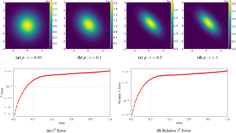
In the 2D case, we consider as follows:
and . The initial condition is set to be the 2D standard Gaussian . The exact solution of Eq. (64) takes the following analytical form [33]
| (66) |
where and . We draw 10000 samples from as the training set. As an advantage of the neural network-based algorithm, we can compute point-wisely through a function composition , where can be computed by solving a convex optimization problem, i.e., . Fig. 5(a) - (d) shows the predicted density on a uniform grid on . The absolute and relative -errors on the grid are shown in Figs. 5(e)-(f). It can be noticed that the relative -error for the predicted solution is around , which is quite accurate given the limited number of samples used.
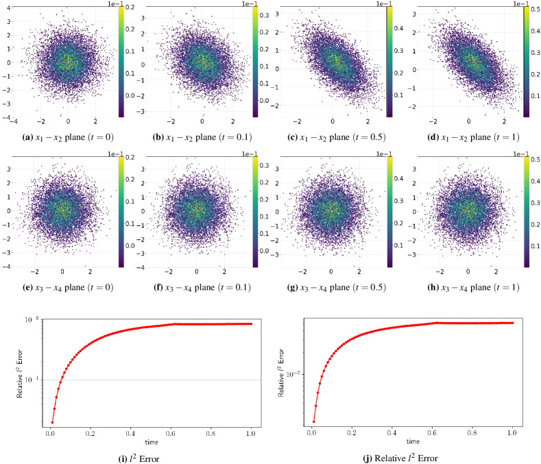
In the 4D case, we take to be
and . The initial condition is set to be a 4D standard normal distribution . The exact solution of Eq. (64) follows the normal distribution with and Here is the direct sum. Same to the 2D case, we draw 10000 initial samples from . Fig. 6 shows the evolution of samples as well the values of the numerical solution on individual samples over space and time. Interestingly, the relative -error in 4D case is similar to the 2D case. The dimension-independent error bound suggests the potential of the current method for handling higher-dimensional problems.
Fokker–Planck type equations have a wide application in machine learning. One of the fundamental tasks in modern statistics and machine learning is to estimate or generate samples from a target distribution , which might be completely known, partially known up to the normalizing constant, or empirically given by samples. Examples include Bayesian inference [7], numerical integration [54], space-filling design [61], density estimation [69], and generative learning [59]. These problems can be transformed as an optimization problem, which is to seek for a by solving an optimization problem
| (67) |
where is the admissible set, is a dissimilarity function that assesses the differences between two probability measures and . The classical dissimilarities include the Kullback–Leibler (KL) divergence and the Maximum Mean Discrepancy (MMD). The optimal solution to the optimization problem can be obtained by solving a Fokker–Planck type equation, given by
| (68) |
The developed numerical approach has potential applications in these machine learning problems.
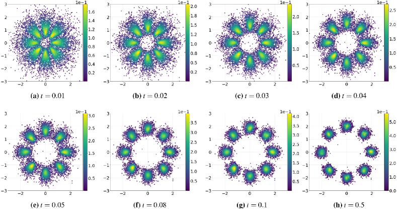
To illustrate this point, we consider a toy problem that is widely used in the machine learning literature [32]. The goal is to sample from a target distribution , which is known up to a normalizing constant. We take the dissimilarity function as the KL divergence then Eq. (68) is reduced to the Fokker–Planck equation (64) with . In the numerical experiment, we take the target distribution , an eight components mixture Gaussian distribution, where , , , , , , , , and . The simulation results are summarized in Fig. 7, in which we first draw 10000 samples from a standard normal distribution and show the distribution of samples as well as their weights at different time. It can be noticed that the proposed neural network-based algorithm can generate a weighted sample for a complicated target distribution.
4.3.2 Porous medium equation
Next, we consider a porous medium equation (PME), where is a constant. The PME is a typical example of nonlinear diffusion equations. One important feature of the PME is that the solution to the PME has a compact support at any time if the initial data has a compact support. The free boundary of the compact support moves outward with a finite speed, known as the property of finite speed propagation [71]. As a consequence, numerical simulations of the PME are often difficult by using Eulerian methods, which may fail to capture the movement of the free boundary and suffer from numerical oscillations [50]. In a recent work [50], the authors developed a variational Lagrangian scheme using a finite element method. Here we show the ability of the Lagrangian EVNN scheme to solve the PME with a free boundary. Following [50], we employ the energy-dissipation law
| (69) |
to develop the EVNN scheme.

We take in the simulation. To test the numerical accuracy of the EVNN scheme for solving the PME, we consider a 2D Barenblatt–Pattle solution to the PME. The Barenblatt–Pattle solution in -dimensional space is given by
| (70) |
where , , and is a constant that is related to the initial mass. This solution is radially symmetric, self-similar, and has compact support for any finite time, where . We take the Barenblatt solution (70) with at as the initial condition, and compare the numerical solution at with the exact solution . We choose as a set of uniform grid points inside a disk . To visualize the numerical results, we also draw points distributed with equal arc length on the initial free boundary and evolve them using the neural network. The numerical results with are shown in Fig. 8. It can be noticed that the proposed neural network-based algorithm can well approximate the Barenblatt–Pattle solution and capture the movement of the free boundary.
We note that the numerical methods to solve generalized diffusions (4) can also be formulated in the Eulerian frame of reference based on the notion of Wasserstein gradient flow [35]. However, it is often challenging to compute the Wasserstein distance between two probability densities efficiently with high accuracy, which often requires solving an additional min-max problem or minimization problem [5, 6, 9, 33]. In a recent study [33], the authors initially employ a fully connected neural network to approximate and subsequently utilize an additional ICNN to calculate the Wasserstein distance between two probability densities. Compared with their approach, our method is indeed more efficient and accurate.
5 Conclusion
In this paper, we develop structure-preserving EVNN schemes for simulating the -gradient flows and the generalized diffusions by utilizing a neural network as a tool for spatial discretization, within the framework of the discrete energetic variational approach. These numerical schemes are directly constructed based on a prescribed continuous energy-dissipation law for the system, without the need for the underlying PDE. The incorporation of mesh-free neural network discretization opens up exciting possibilities for tackling high-dimensional gradient flows arising in different applications in the future.
Various numerical experiments are presented to demonstrate the accuracy and energy stability of the proposed numerical scheme. In our future work, we will explore the effects of different neural network architectures, sampling strategies, and optimization methods, followed by a detailed numerical analysis. Additionally, we intend to employ the EVNN scheme to investigate other complex fluid models, including the Cahn–Hilliard equation and Cahn–Hilliard–Navier–Stokes equations, as well as solve machine learning problems such as generative modeling and density estimation.
Acknowledgments
C. L and Y. W were partially supported by NSF DMS-1950868 and DMS-2153029. Z. X was partially supported by the NSF CDS&E-MSS 1854779.
References
- [1] S. Adams, N. Dirr, M. Peletier, and J. Zimmer, Large deviations and gradient flows, Philosophical Transactions of the Royal Society A: Mathematical, Physical and Engineering Sciences, 371 (2013), p. 20120341.
- [2] B. Amos, L. Xu, and J. Z. Kolter, Input convex neural networks, in International Conference on Machine Learning, PMLR, 2017, pp. 146–155.
- [3] A. Baron, Universal approximation bounds for superposition of a sigmoid function, IEEE Transaction on Information Theory, 39 (1993), pp. 930–945.
- [4] R. Bellman, Dynamic Programming, Dover Publications, 1957.
- [5] J.-D. Benamou and Y. Brenier, A computational fluid mechanics solution to the Monge-Kantorovich mass transfer problem, Numerische Mathematik, 84 (2000), pp. 375–393.
- [6] J.-D. Benamou, G. Carlier, and M. Laborde, An augmented lagrangian approach to wasserstein gradient flows and applications, ESAIM: Proceedings and surveys, 54 (2016), pp. 1–17.
- [7] D. M. Blei, A. Kucukelbir, and J. D. McAuliffe, Variational inference: A review for statisticians, J. Am. Stat. Assoc., 112 (2017), pp. 859–877.
- [8] J. Bruna, B. Peherstorfer, and E. Vanden-Eijnden, Neural galerkin scheme with active learning for high-dimensional evolution equations, arXiv preprint arXiv:2203.01360, (2022).
- [9] J. A. Carrillo, K. Craig, L. Wang, and C. Wei, Primal dual methods for wasserstein gradient flows, Foundations of Computational Mathematics, 22 (2022), pp. 389–443.
- [10] G. Cybenko, Approximation by superpositions of a sigmoidal function, Mathematics of control, signals and systems, 2 (1989), pp. 303–314.
- [11] P.-G. De Gennes and J. Prost, The physics of liquid crystals, no. 83, Oxford university press, 1993.
- [12] J. Devlin, M.-W. Chang, K. Lee, and K. Toutanova, Bert: Pre-training of deep bidirectional transformers for language understanding, arXiv preprint arXiv:1810.04805, (2018).
- [13] T. Dockhorn, A discussion on solving partial differential equations using neural networks, arXiv preprint arXiv:1904.07200, (2019).
- [14] M. Doi, Onsager’s variational principle in soft matter, J. Phys.: Condens. Matter, 23 (2011), p. 284118.
- [15] Q. Du and X. Feng, The phase field method for geometric moving interfaces and their numerical approximations, Handbook of Numerical Analysis, 21 (2020), pp. 425–508.
- [16] Y. Du and T. A. Zaki, Evolutional deep neural network, Phys. Rev. E, 104 (2021), p. 045303.
- [17] C. Durkan, A. Bekasov, I. Murray, and G. Papamakarios, Neural spline flows, Advances in neural information processing systems, 32 (2019).
- [18] W. E, J. Han, and A. Jentzen, Algorithms for solving high dimensional pdes: From nonlinear Monte Carlo to machine learning, Nonlinearity, 35 (2021), p. 278.
- [19] W. E, C. Ma, and L. Wu, Machine learning from a continuous viewpoint, i, Science China Mathematics, 63 (2020), pp. 2233––2266.
- [20] W. E, C. Ma, L. Wu, and S. Wojtowytsch, Towards a mathematical understanding of neural network-based machine learning: What we know and what we don’t, CSIAM Transactions on Applied Mathematics, 1 (2020), pp. 561–615.
- [21] W. E and B. Yu, The deep ritz method: A deep learning-based numerical algorithm for solving variational problems, Communications in Mathematics and Statistics, 6 (2018).
- [22] B. Eisenberg, Y. Hyon, and C. Liu, Energy variational analysis of ions in water and channels: Field theory for primitive models of complex ionic fluids, The Journal of Chemical Physics, 133 (2010), p. 104104.
- [23] J. L. Ericksen, Introduction to the Thermodynamics of Solids, vol. 275, Springer, 1998.
- [24] M.-H. Giga, A. Kirshtein, and C. Liu, Variational modeling and complex fluids, Handbook of mathematical analysis in mechanics of viscous fluids, (2017), pp. 1–41.
- [25] E. D. Giorgi, Movimenti minimizzanti, in Proceedings of the Conference on Aspetti e problemi della Matematica oggi, Lecce, 1992.
- [26] X. Glorot and Y. Bengio, Understanding the difficulty of training deep feedforward neural networks, in Proceedings of the thirteenth international conference on artificial intelligence and statistics, JMLR Workshop and Conference Proceedings, 2010, pp. 249–256.
- [27] J. Han, A. Jentzen, and W. E, Solving high-dimensional partial differential equations using deep learning, Proceedings of the National Academy of Sciences, 115 (2018), pp. 8505–8510.
- [28] B. Hanin, Which neural net architectures give rise to exploding and vanishing gradients?, in NeurIPS, 2018.
- [29] K. He, X. Zhang, S. Ren, and J. Sun, Deep residual learning for image recognition, in Proceedings of the IEEE conference on computer vision and pattern recognition, 2016, pp. 770–778.
- [30] , Identity mappings in deep residual networks, in European conference on computer vision, Springer, 2016, pp. 630–645.
- [31] G. Hinton, L. Deng, D. Yu, G. E. Dahl, A.-r. Mohamed, N. Jaitly, A. Senior, V. Vanhoucke, P. Nguyen, T. N. Sainath, et al., Deep neural networks for acoustic modeling in speech recognition: The shared views of four research groups, IEEE Signal processing magazine, 29 (2012), pp. 82–97.
- [32] C.-W. Huang, R. T. Chen, C. Tsirigotis, and A. Courville, Convex potential flows: Universal probability distributions with optimal transport and convex optimization, arXiv preprint arXiv:2012.05942, (2020).
- [33] H. J. Hwang, C. Kim, M. S. Park, and H. Son, The deep minimizing movement scheme, arXiv preprint arXiv:2109.14851, (2021).
- [34] K. Jiang and P. Zhang, Numerical methods for quasicrystals, J. Comput. Phys., 256 (2014), pp. 428–440.
- [35] R. Jordan, D. Kinderlehrer, and F. Otto, The variational formulation of the Fokker–Planck equation, SIAM J. Math. Anal., 29 (1998), pp. 1–17.
- [36] E. F. Keller and L. A. Segel, Initiation of slime mold aggregation viewed as an instability, Journal of theoretical biology, 26 (1970), pp. 399–415.
- [37] E. Kharazmi, Z. Zhang, and G. E. Karniadakis, hp-vpinns: Variational physics-informed neural networks with domain decomposition, Computer Methods in Applied Mechanics and Engineering, 374 (2021), p. 113547.
- [38] Y. Khoo, J. Lu, and L. Ying, Solving parametric PDE problems with artificial neural networks, European Journal of Applied Mathematics, 32 (2021), pp. 421–435.
- [39] D. P. Kingma, T. Salimans, R. Jozefowicz, X. Chen, I. Sutskever, and M. Welling, Improved variational inference with inverse autoregressive flow, Advances in neural information processing systems, 29 (2016).
- [40] J. F. Kolen and S. C. Kremer, Gradient Flow in Recurrent Nets: The Difficulty of Learning LongTerm Dependencies, 2001, pp. 237–243.
- [41] A. Krizhevsky, I. Sutskever, and G. E. Hinton, Imagenet classification with deep convolutional neural networks, in Advances in neural information processing systems, 2012, pp. 1097–1105.
- [42] I. E. Lagaris, A. Likas, and D. I. Fotiadis, Artificial neural networks for solving ordinary and partial differential equations, IEEE transactions on neural networks, 9 (1998), pp. 987–1000.
- [43] Y. LeCun, L. Bottou, Y. Bengio, and P. Haffner, Gradient-based learning applied to document recognition, Proceedings of the IEEE, 86 (1998), pp. 2278–2324.
- [44] R. Lifshitz and H. Diamant, Soft quasicrystals–why are they stable?, Philosophical Magazine, 87 (2007), pp. 3021–3030.
- [45] F. H. Lin and C. Liu, Static and dynamic theories of liquid crystals, J. Partial Differential Equations, 14 (2001), pp. 289–330.
- [46] S. Lisini, D. Matthes, and G. Savaré, Cahn–Hilliard and thin film equations with nonlinear mobility as gradient flows in weighted-wasserstein metrics, Journal of differential equations, 253 (2012), pp. 814–850.
- [47] G. Litjens, T. Kooi, B. E. Bejnordi, A. A. A. Setio, F. Ciompi, M. Ghafoorian, J. A. Van Der Laak, B. Van Ginneken, and C. I. Sánchez, A survey on deep learning in medical image analysis, Medical image analysis, 42 (2017), pp. 60–88.
- [48] C. Liu and H. Sun, On energetic variational approaches in modeling the nematic liquid crystal flows, Discrete & Continuous Dynamical Systems, 23 (2009), p. 455.
- [49] C. Liu, C. Wang, and Y. Wang, A structure-preserving, operator splitting scheme for reaction-diffusion equations with detailed balance, Journal of Computational Physics, 436 (2021), p. 110253.
- [50] C. Liu and Y. Wang, On lagrangian schemes for porous medium type generalized diffusion equations: a discrete energetic variational approach, J. Comput. Phys., 417 (2020), p. 109566.
- [51] , A variational lagrangian scheme for a phase-field model: A discrete energetic variational approach, SIAM J. Sci. Comput., 42 (2020), pp. B1541–B1569.
- [52] L. Lu, X. Meng, Z. Mao, and G. E. Karniadakis, Deepxde: A deep learning library for solving differential equations, SIAM Review, 63 (2021), pp. 208–228.
- [53] Y. Lu, J. Lu, and M. Wang, A priori generalization analysis of the deep ritz method for solving high dimensional elliptic partial differential equations, in Conference on Learning Theory, PMLR, 2021, pp. 3196–3241.
- [54] T. Müller, B. McWilliams, F. Rousselle, M. Gross, and J. Novák, Neural importance sampling, ACM Transactions on Graphics (TOG), 38 (2019), pp. 1–19.
- [55] J. Noh, Y. Wang, H.-L. Liang, V. S. R. Jampani, A. Majumdar, and J. P. Lagerwall, Dynamic tuning of the director field in liquid crystal shells using block copolymers, Phys. Rev. Res., 2 (2020), p. 033160.
- [56] T. Ohta and K. Kawasaki, Equilibrium morphology of block copolymer melts, Macromolecules, 19 (1986), pp. 2621–2632.
- [57] L. Onsager, Reciprocal relations in irreversible processes. I., Phys. Rev., 37 (1931), p. 405.
- [58] , Reciprocal relations in irreversible processes. II., Phys. Rev., 38 (1931), p. 2265.
- [59] G. Papamakarios, E. T. Nalisnick, D. J. Rezende, S. Mohamed, and B. Lakshminarayanan, Normalizing flows for probabilistic modeling and inference., J. Mach. Learn. Res., 22 (2021), pp. 1–64.
- [60] M. A. Peletier, Variational modelling: Energies, gradient flows, and large deviations, arXiv preprint arXiv:1402.1990, (2014).
- [61] L. Pronzato and W. G. Müller, Design of computer experiments: space filling and beyond, Statistics and Computing, 22 (2012), pp. 681–701.
- [62] M. Raissi, P. Perdikaris, and G. E. Karniadakis, Physics informed deep learning (part i): Data-driven solutions of nonlinear partial differential equations, arXiv preprint arXiv:1711.10561, (2017).
- [63] L. Rayleigh, Some general theorems relating to vibrations, Proceedings of the London Mathematical Society, 4 (1873), pp. 357–368.
- [64] D. Rezende and S. Mohamed, Variational inference with normalizing flows, in International conference on machine learning, PMLR, 2015, pp. 1530–1538.
- [65] G. M. Rotskoff, A. R. Mitchell, and E. Vanden-Eijnden, Active importance sampling for variational objectives dominated by rare events: Consequences for optimization and generalization, arXiv preprint arXiv:2008.06334, (2020).
- [66] A. J. Salgado and S. M. Wise, Classical Numerical Analysis: A Comprehensive Course, Cambridge University Press, 2022.
- [67] Z. Shen, H. Yang, and S. Zhang, Nonlinear approximation via compositions, arXiv preprint arXiv:1902.10170, (2019).
- [68] J. Sirignano and K. Spiliopoulos, Dgm: A deep learning algorithm for solving partial differential equations, J. Comput. Phys., 375 (2018), pp. 1339–1364.
- [69] E. G. Tabak, E. Vanden-Eijnden, et al., Density estimation by dual ascent of the log-likelihood, Communications in Mathematical Sciences, 8 (2010), pp. 217–233.
- [70] B. P. van Milligen, V. Tribaldos, and J. Jiménez, Neural network differential equation and plasma equilibrium solver, Phys. Rev. Lett., 75 (1995), p. 3594.
- [71] J. L. Vázquez, The porous medium equation: mathematical theory, Oxford University Press, 2007.
- [72] H. Wang, T. Qian, and X. Xu, Onsager’s variational principle in active soft matter, Soft Matter, 17 (2021), pp. 3634–3653.
- [73] Y. Wang, J. Chen, C. Liu, and L. Kang, Particle-based energetic variational inference, Stat. Comput., 31 (2021), pp. 1–17.
- [74] Y. Wang and C. Liu, Some recent advances in energetic variational approaches, Entropy, 24 (2022).
- [75] Y. Wang, C. Liu, P. Liu, and B. Eisenberg, Field theory of reaction-diffusion: Law of mass action with an energetic variational approach, Phys. Rev. E, 102 (2020), p. 062147.
- [76] Y. Wang, T.-F. Zhang, and C. Liu, A two species micro–macro model of wormlike micellar solutions and its maximum entropy closure approximations: An energetic variational approach, Journal of Non-Newtonian Fluid Mechanics, 293 (2021), p. 104559.
- [77] Q. Wei, Y. Jiang, and J. Z. Y. Chen, Machine-learning solver for modified diffusion equations, Phys. Rev. E, 98 (2018), p. 053304.
- [78] E. Weinan, Machine learning and computational mathematics, arXiv preprint arXiv:2009.14596, (2020).
- [79] J. Xu, Y. Li, S. Wu, and A. Bousquet, On the stability and accuracy of partially and fully implicit schemes for phase field modeling, Computer Methods in Applied Mechanics and Engineering, 345 (2019), pp. 826–853.
- [80] S. Xu, P. Sheng, and C. Liu, An energetic variational approach for ion transport, Communications in Mathematical Sciences, 12 (2014), pp. 779–789.
- [81] S. Xu, Z. Xu, O. V. Kim, R. I. Litvinov, J. W. Weisel, and M. S. Alber, Model predictions of deformation, embolization and permeability of partially obstructive blood clots under variable shear flow, Journal of The Royal Society Interface, 14 (2017).
- [82] X. Xu, Y. Di, and M. Doi, Variational method for liquids moving on a substrate, Physics of Fluids, 28 (2016), p. 087101.
- [83] P. Yue, J. J. Feng, C. Liu, and J. Shen, A diffuse-interface method for simulating two-phase flows of complex fluids, J. Fluid Mech., 515 (2004), pp. 293–317.
- [84] Y. Zang, G. Bao, X. Ye, and H. Zhou, Weak adversarial networks for high-dimensional partial differential equations, J. Comput. Phys., 411 (2020), p. 109409.