Energetic Resilience of Linear Driftless Systems

Ram Padmanabhan and Melkior Ornik This work was supported by Air Force Office of Scientific Research grant FA9550-23-1-0131 and NASA University Leadership Initiative grant 80NSSC22M0070. (Corresponding Author: Ram Padmanabhan)The authors are with the University of Illinois Urbana-Champaign, Urbana, IL 61801, USA. Emails: {ramp3, mornik}@illinois.edu

Abstract

When a malfunction causes a control system to lose authority over a subset of its actuators, achieving a task may require spending additional energy in order to compensate for the effect of uncontrolled inputs. To understand this increase in energy, we introduce energetic resilience metrics that quantify the maximal additional energy required to achieve finite-time regulation in linear driftless systems that lose authority over some of their actuators. We first derive optimal control signals and minimum energies to achieve this task in both the nominal and malfunctioning systems. We then obtain a bound on the worst-case energy used by the malfunctioning system, and its exact expression in the special case of loss of authority over one actuator. Further considering this special case, we derive bounds on additive and multiplicative metrics for energetic resilience. A simulation example on a model of an underwater robot demonstrates that these bounds are useful in quantifying the increased energy used by a system suffering a partial loss of control authority.

I Introduction

Control systems can suffer from a wide variety of failures, either due to system faults or adversarial attacks. Depending on their nature, failures can prevent a system from achieving a specific performance objective, including reachability or safety, even if mitigating actions are taken. Informally, a system is said to be resilient if its objectives can be achieved despite a failure. A well-publicized example of a failure was when the Nauka module docked to the International Space Station (ISS) in 2021. A software error resulted in an unexpected firing of the module’s thrusters, tilting the ISS from its nominal position for $47$ minutes by up to $540^{\circ}$ , described as a “loss of attitude control” by the National Aeronautics and Space Administration (NASA) [1]. The failure mode in this event was that of partial loss of control authority, where the system lost authority over some of its thrusters, and other thrusters on the ISS had to be used to counteract the effect of the uncontrolled thrust.

Motivated by this example, in this paper, we consider systems that are affected by complete loss in control authority over a subset of their actuators. In such a system, the uncontrolled inputs, potentially chosen by an adversary, can take on any values in the input space. However, these uncontrolled inputs are measurable, and can be used by the controlled inputs — under the authority of the system — in order to achieve a task. Such actuator faults are the most common cause of failure in spacecraft attitude control systems, accounting for around $44\%$ of all faults [2, 3]. While building redundancy in actuators [4, 5] or using control reconfiguration schemes [5, 6, 3] can aid resilience, this techniques can result in prohibitively high costs in control design.

Addressing this problem with classical control methods is bound to fail. Standard fault-tolerant control theories consider only limited actuator failure modes, such as actuators “locked” into producing constant inputs [7], or actuators with reduced effectiveness that remain controllable [8, 9]. Under a loss of control authority, uncontrolled inputs can take on values with the same magnitude as the controlled inputs, leading to the failure of robust control techniques [10] which require external disturbances to have much smaller magnitudes than the controlled inputs [11]. The uncontrolled inputs can also change significantly in a short period of time, leading to the failure of adaptive control strategies [11, 12].

In [13], Bouvier and Ornik derived conditions for the resilient reachability of linear systems, i.e., reachability of a target set under any uncontrolled inputs. These conditions were used in [10] to design controllers that enable linear systems to achieve a target despite this malfunction. To quantify the additional time it may take for a target to be reached under a loss of control authority, Bouvier et al. introduced the notion of quantitative resilience in [14]. Quantitative resilience was defined as the maximal ratio of minimum reach times to achieve a target for a nominal system and a malfunctioning system. While initially defined for linear driftless systems in [14], this definition was extended to general linear systems in [15, 16].

In this paper, we introduce metrics for a similar quantitative notion called energetic resilience. Instead of considering minimal reach times for the nominal and malfunctioning systems as in the works of [14] and [16], we consider the minimal control energies required to achieve drive the state to the origin from an initial condition, in a given finite time. In practical systems, the maximal additional control energy required to achieve this task is directly related to maximal consumption of additional resources, such as fuel in vehicular systems. Quantifying this is important in understanding the maximum capacity of resources required. Designing this resource capacity must take into account all possible malfunctioning inputs, which is not a straightforward problem. Considering minimal control energies instead of minimal reach times allows us to derive optimal control signals that achieve the task in both the nominal and malfunctioning driftless systems, which was not accomplished by [14, 10, 16]. We also derive a closed-form expression for the worst-case uncontrolled input that seeks to maximize the energy used by the malfunctioning system, which is not provided in the earlier works. Similar metrics were used to quantify the maximal cost of disturbance by [17], considering linear systems affected by external bounded disturbances with no bounds on the control inputs. In contrast to [17], in our setting of partial loss of control authority, the controlled inputs are bounded, and uncontrolled inputs can take on values with the same magnitude. As a preliminary step towards studying the energetic resilience of general linear and nonlinear systems, we focus on linear driftless systems in this paper. Despite their simplicity, driftless dynamics are sufficiently rich to characterize a variety of robotic and underwater systems [18, 19].

The contributions of this paper are organized as follows. In Section II, we formulate the problem statement, providing the definitions of key quantities derived in this paper. Section III discusses the optimal control signals, minimal control energies and restrictions on the time required to achieve a task in both the nominal and malfunctioning systems. These results use a technical lemma that is proved using the calculus of variations. Further, we also consider the worst-case control energy for the malfunctioning system over all possible uncontrolled inputs, and derive an upper bound for this quantity. We conclude Section III by briefly considering the problem of final time design, i.e., choosing a task completion time that minimizes the control energy in the malfunctioning system. In Section IV, we consider the special case of losing authority over one actuator, deriving an exact expression for the worst-case control energy for the malfunctioning system, as well as the worst-case uncontrolled input achieving this energy. We also derive bounds on additive and multiplicative metrics for energetic resilience, both of which quantify how much additional control energy is used by the malfunctioning system compared to the nominal system. In Section V, we consider a model of an underwater robot and illustrate the applicability of our results. In particular, we present the two energetic resilience metrics as a function of distance of the initial condition from the origin, and show that these metrics accurately characterize the additional control energy used by the malfunctioning system.

I-A Notation and Facts

The set $\mathbb{R}^{+}\coloneqq[0,\infty)$ is the set of all non-negative real numbers. For scalars $z\in\mathbb{R}$ , define the $\operatorname*{sign}(\cdot)$ function as $\operatorname*{sign}(z)=z/|z|\in\{-1,+1\}$ if $z\neq 0$ , with $\operatorname*{sign}(0)=0$ . For vectors $z\in\mathbb{R}^{n}$ , the $\operatorname*{sign}(\cdot)$ function operates elementwise on $z$ . The $p$ -norm of a vector $x\in\mathbb{R}^{n}$ is defined as $\|x\|_{p}\coloneqq\left(\sum_{i=1}^{n}|x_{i}|^{p}\right)^{1/p}$ , with $\|x\|_{\infty}\coloneqq\max_{i}|x_{i}|$ . For a matrix $L\in\mathbb{R}^{p\times q}$ with entries indexed $l_{ij}$ , define the induced matrix norms $\|L\|_{1}\coloneqq\max_{j}\sum_{i=1}^{p}|l_{ij}|$ and $\|L\|_{\infty}\coloneqq\max_{i}\sum_{j=1}^{q}|l_{ij}|$ . The Moore-Penrose inverse [20], also called the pseudoinverse of $L$ , is denoted $L^{\dagger}$ . For a continuous function $u:[0,t_{f}]\to\mathbb{R}^{p}$ , the $\mathcal{L}_{2}$ norm is defined as $\|u\|_{\mathcal{L}_{2}}\coloneqq\sqrt{\int_{t=0}^{t_{f}}\|u(t)\|_{2}^{2}\leavevmode\nobreak\ \mathrm{d}t}$ .

For any two matrices $M$ and $N$ such that their product $MN$ can be defined, the sub-multiplicative property of matrix norms is written as $\|MN\|\leq\|M\|\|N\|$ , where $\|.\|$ is any induced norm. For any two vectors $x\in\mathbb{R}^{n}$ and $y\in\mathbb{R}^{n}$ , the Cauchy-Schwarz inequality can be written as $|x^{T}y|\leq\|x\|_{2}\|y\|_{2}$ . The minimum and maximum eigenvalues of a symmetric matrix $P\in\mathbb{R}^{n\times n}$ are denoted $\lambda_{\min}(P)$ and $\lambda_{\max}(P)$ . For such a matrix, the Rayleigh inequality [21] $\lambda_{\min}(P)\|x\|_{2}^{2}\leq x^{T}Px\leq\lambda_{\max}(P)\|x\|_{2}^{2}$ holds for any vector $x\in\mathbb{R}^{n}$ .

II Problem Formulation

In this paper, we consider linear driftless systems of the form

\dot{x}(t)=Bu(t),\leavevmode\nobreak\ \leavevmode\nobreak\ x(0)=x_{0}\neq 0,

(1)

where $x(t)\in\mathbb{R}^{n}$ is the state, $u(t)\in\mathbb{R}^{m+p}$ is the control and $B\in\mathbb{R}^{n\times(m+p)}$ is the input matrix. The set of admissible controls $\operatorname*{\mathcal{U}}$ is defined as:

\operatorname*{\mathcal{U}}\coloneqq\left\{u:\mathbb{R}^{+}\to\mathbb{R}^{m+p}:\|u(t)\|_{\infty}\leq 1\leavevmode\nobreak\ \text{ for all $t$}\right\},

(2)

in line with prior work [16, 22]. We consider malfunctions that result in the system losing control authority over $p$ of its $m+p$ actuators. Then, the matrix $B$ and control $u(t)$ can be split into controlled and uncontrolled components, and the malfunctioning system can be written as:

\dot{x}(t)=\begin{bmatrix}B_{c}&&B_{uc}\end{bmatrix}\begin{bmatrix}u_{c}(t)\\ u_{uc}(t)\end{bmatrix}=B_{c}u_{c}(t)+B_{uc}u_{uc}(t),

(3)

where the subscripts $c$ and $uc$ denote controlled and uncontrolled respectively. Here, $B=[B_{c},B_{uc}]$ , $B_{c}\in\mathbb{R}^{n\times m}$ , $B_{uc}\in\mathbb{R}^{n\times p}$ , $u_{c}(t)\in\mathbb{R}^{m}$ and $u_{uc}(t)\in\mathbb{R}^{p}$ . Based on the set of admissible controls $\operatorname*{\mathcal{U}}$ in (2), we have $u_{c}\in\operatorname*{\mathcal{U}_{c}}$ and $u_{uc}\in\operatorname*{\mathcal{U}_{uc}}$ , where


$\displaystyle\operatorname*{\mathcal{U}_{c}}$	$\displaystyle\coloneqq\left\{u_{c}:\mathbb{R}^{+}\to\mathbb{R}^{m}:\\|u_{c}(t)\\|_{\infty}\leq 1\leavevmode\nobreak\ \text{for all $t$}\right\},$	(4a)
$\displaystyle\operatorname*{\mathcal{U}_{uc}}$	$\displaystyle\coloneqq\left\{u_{uc}:\mathbb{R}^{+}\to\mathbb{R}^{p}:\\|u_{uc}(t)\\|_{\infty}\leq 1\leavevmode\nobreak\ \text{for all $t$}\right\}.$	(4b)

In this setting, the system has authority over the controlled input $u_{c}$ , but the uncontrolled input $u_{uc}$ can be chosen arbitrarily from the space $\operatorname*{\mathcal{U}_{uc}}$ , potentially by an adversary. However, this uncontrolled input is observable, and hence can be used in the design of $u_{c}$ .

Our objective is the task of finite-time regulation, achieving $x(t_{f})=0$ for a specified final time $t_{f}$ . In the nominal case, this task is achieved using the input $u\in\operatorname*{\mathcal{U}}$ , while in the malfunctioning case, this task must be achieved using only the controlled input $u_{c}\in\operatorname*{\mathcal{U}_{c}}$ , for any given uncontrolled inputs $u_{uc}\in\operatorname*{\mathcal{U}_{uc}}$ . In this context, we define the notion of finite-time stabilizing resilience of a system, adapted from [14].

Definition 1 (Finite-time Stabilizing Resilience).

A system (1) is resilient to the loss of control authority over $p$ of its actuators, represented by the matrix $B_{uc}$ if, for all uncontrolled inputs $u_{uc}\in\operatorname*{\mathcal{U}_{uc}}$ and for a given final time $t_{f}$ , there exists a controlled input $u_{c}\in\operatorname*{\mathcal{U}_{c}}$ such that the system achieves the objective of finite-time regulation, i.e. $x(t_{f})=0$ .

A system may be finite-time stabilizing resilient for some final times $t_{f}$ and not resilient for other final times. Throughout the rest of this paper, we refer to finite-time stabilizing resilience as simply resilience. We also assume that the nominal dynamics (1) are controllable, i.e., that finite-time regulation can be achieved from any initial state $x_{0}$ . In both the nominal and malfunctioning cases, we are interested in the minimal control energies to achieve this task. Achieving this task might require considerably more control energy in the malfunctioning case compared to the nominal case. We thus aim to quantify the maximal additional control energy used by the malfunctioning system over all possible uncontrolled inputs $u_{uc}$ , compared to the nominal system. To this end, we make the following definitions.

Definition 2 (Nominal Energy).

The nominal energy is the minimum energy in the input $u$ required to achieve finite-time regulation in time $t_{f}$ from the initial condition $x_{0}\neq 0$ , following the nominal dynamics (1):

E_{N}^{*}(x_{0},t_{f})\coloneqq\inf_{u\in\operatorname*{\mathcal{U}}}\left\{\left\|u\right\|_{\mathcal{L}_{2}}^{2}\leavevmode\nobreak\ \text{s.t. $x(t_{f})=0$ using \eqref{eq:Nominal}}\right\}.

(5)

Definition 3 (Malfunctioning Energy).

The malfunctioning energy is the minimum energy in the controlled input $u_{c}$ required to achieve finite-time regulation in time $t_{f}$ from the initial condition $x_{0}\neq 0$ , for a given uncontrolled input $u_{uc}$ , following the malfunctioning dynamics (3):

	$\displaystyle E_{M}^{*}(x_{0},t_{f},u_{uc})$	$\displaystyle\coloneqq\inf_{u_{c}(u_{uc})\in\operatorname*{\mathcal{U}_{c}}}\Bigl{\{}\left\\|u_{c}(u_{uc})\right\\|_{\mathcal{L}_{2}}^{2}$
		$\displaystyle\leavevmode\nobreak\ \text{s.t. $x(t_{f})=0$ in \eqref{eq:Malfunctioning}, for the given $u_{uc}$}\Bigr{\}},$		(6)

where $u_{c}(u_{uc})$ explicitly provides the dependence of the controlled input $u_{c}:\mathbb{R}^{+}\to\mathbb{R}^{m}$ on the uncontrolled input $u_{uc}$ , with a slight abuse of notation.

Definition 4 (Total Energy).

The total energy is the energy used by all inputs of the malfunctioning system (3) for a given uncontrolled input $u_{uc}$ , when the optimal controlled input $u_{c}(u_{uc})$ in (6) is used. In other words,

E_{M}^{+}(x_{0},t_{f},u_{uc})\coloneqq E_{M}^{*}(x_{0},t_{f},u_{uc})+\left\|u_{uc}\right\|_{\mathcal{L}_{2}}^{2}.

(7)

Definition 5 (Worst-case Total Energy).

The worst-case total energy is the maximal total energy (7) over all possible uncontrolled inputs $u_{uc}$ :

	$\displaystyle\overline{E}_{M}(x_{0},t_{f})$	$\displaystyle=\sup_{u_{uc}\in\operatorname*{\mathcal{U}_{uc}}}E_{M}^{+}(x_{0},t_{f},u_{uc})$
		$\displaystyle=\sup_{u_{uc}\in\operatorname{\mathcal{U}_{uc}}}\left\{E_{M}^{}(x_{0},t_{f},u_{uc})+\left\\|u_{uc}\right\\|_{\mathcal{L}_{2}}^{2}\right\}$		(8)

The worst-case total energy quantifies the maximal effect of the uncontrolled input $u_{uc}$ on the overall control energy used by the system.

The overarching aim of this paper is to understand how much larger the worst-case total energy is, compared to the nominal energy. This is quantified by the following energetic resilience metrics, similar to those defined in [17].

Definition 6 (Additive Energetic Resilience).

For an initial condition $x_{0}$ no farther than a distance of $R$ from the origin, we define the additive energetic resilience of system (1) as

r_{A}(t_{f},R)\coloneqq\sup_{\|x_{0}\|_{2}\leq R}\left\{\overline{E}_{M}(x_{0},t_{f})-E_{N}^{*}(x_{0},t_{f})\right\}.

(9)

Definition 7 (Multiplicative Energetic Resilience).

For an initial condition at a distance of at least $R$ from the origin, we define the multiplicative energetic resilience of system (1) as

r_{M}(t_{f},R)\coloneqq\inf_{\|x_{0}\|_{2}\geq R}\frac{E_{N}^{*}(x_{0},t_{f})}{\overline{E}_{M}(x_{0},t_{f})}.

(10)

Using (9), the malfunctioning system will use at most $r_{A}(t_{f},R)$ more energy than the nominal system to achieve finite-time regulation from an initial condition $x_{0}$ no farther than $R$ from the origin, and for a given $t_{f}$ . We are thus interested in an upper bound for this metric. The constraint $\|x_{0}\|_{2}\leq R$ is required to ensure that this metric takes on a finite value. Similarly, (10) is a multiplicative measure of the increased energy required. For instance, if $r_{A}(t_{f},R)\geq 1/2$ , then the actuators of the malfunctioning system use at most twice the energy used by the actuators of the nominal system to achieve finite-time regulation, for a given $t_{f}$ and $R$ . We are thus interested in a lower bound for this metric. Without the constraint $\|x_{0}\|_{2}\geq R$ , $x_{0}$ can be arbitrarily close to the origin and so can $E_{N}^{*}(x_{0},t_{f})$ , reducing the metric to $0$ . We note that the definition of $r_{M}(t_{f},R)$ is closely related to the definition of quantitative resilience defined by Bouvier et al. for driftless systems in [14] and for general linear systems in [16]. However, quantitative resilience was defined based on reachable time while our definitions consider the control energy.

In the following section, we derive closed-form expressions for the nominal and malfunctioning energy, as well as a bound on the worst-case total energy. To quantify the maximal additional energy used by the malfunctioning system compared to the nominal system, we compare the quantities $E_{N}^{*}(x_{0},t_{f})$ from (5) and $\overline{E}_{M}(x_{0},t_{f})$ from (8). This comparison is achieved in Section IV by deriving bounds on the energetic resilience metrics (9) and (10), for the special case of losing authority over a single actuator.

III Nominal and Malfunctioning Energies

In this section, we derive expressions for the three quantities defined in Section II, as well as the corresponding optimal control inputs. We also briefly discuss a problem of final time design for the malfunctioning system, which finds the optimal final time that minimizes the malfunctioning energy for a given uncontrolled input.

Next, we present a lemma which is central to the development in this section.

Lemma 1.

Let $\mathcal{Z}$ be a set of continuous, real vector-valued functions with a given mean value $\overline{z}$ in the interval $[0,t_{f}]$ , i.e.

\mathcal{Z}\coloneqq\left\{z:[0,t_{f}]\to\mathbb{R}^{n_{z}}:\frac{1}{t_{f}}\int_{0}^{t_{f}}z(t)\mathrm{d}t=\overline{z}\in\mathbb{R}^{n_{z}}\right\}.

Let $z^{*}(t)$ denote the signal with the minimum energy in $\mathcal{Z}$ , i.e. $z^{*}\coloneqq\operatorname*{arg\,min}_{z\in\mathcal{Z}}\int_{0}^{t_{f}}z^{T}(t)z(t)\mathrm{d}t.$ Then,

z^{*}(t)=\overline{z}\leavevmode\nobreak\ \text{ for all $t\in[0,t_{f}]$.}

In other words, over all signals with a given mean value, the signal with the minimum energy is a constant equal to that mean value for all time.

Proof.

We wish to find the solution of the following problem:

	$\displaystyle\operatorname*{arg\,min}_{z}$	$\displaystyle\int_{0}^{t_{f}}z^{T}(t)z(t)\mathrm{d}t$
	$\displaystyle\text{s.t. }\leavevmode\nobreak\ \frac{1}{t_{f}}$	$\displaystyle\int_{0}^{t_{f}}z(t)\mathrm{d}t=\overline{z}$

for a given $\overline{z}\in\mathbb{R}^{n_{z}}$ . This is a constrained calculus of variations problem [23]. Let $L(t,z)=z^{T}(t)z(t)$ and $M(t,z)=z(t)$ . The first-order necessary condition for optimality states that the solution $z^{*}(t)$ must satisfy the Euler-Lagrange equation for $\lambda_{0}^{*}L(t,z)+\lambda^{*T}M(t,z)$ for $(\lambda_{0}^{*},\lambda^{*})\neq(0,0)$ [23]. Thus,

		$\displaystyle{\frac{\partial}{\partial z}\left(\lambda_{0}^{}z^{T}(t)z^{}(t)+\lambda^{T}z^{*}(t)\right)}$
	$\displaystyle=$	$\displaystyle{\frac{d}{dt}\left[\frac{\partial}{\partial z^{\prime}}\left(\lambda_{0}^{}z^{T}(t)z^{}(t)+\lambda^{T}z^{*}(t)\right)\right]=0,}$

where the last equality holds since $L(t,z)$ and $M(t,z)$ are independent of $z^{\prime}=\frac{dz}{dt}$ . Then, $z^{*}(t)$ satisfies

\lambda_{0}^{*}z^{*}(t)+\lambda^{*}=0.

If $\lambda_{0}^{*}=0$ , then $\lambda^{*}=0$ , contradicting the requirement that $(\lambda_{0}^{*},\lambda^{*})\neq(0,0)$ . Thus, $\lambda_{0}^{*}\neq 0$ , and

z^{*}(t)=-\frac{\lambda^{*}}{\lambda_{0}^{*}},

i.e. a constant. Given the constraint $\frac{1}{t_{f}}\int_{0}^{t_{f}}z(t)=\overline{z}$ , we have $z^{*}(t)=\overline{z}\leavevmode\nobreak\ \text{ for all $t\in[0,t_{f}]$.}$ ∎

Armed with this result, we first derive a closed-form expression for the nominal energy.

III-A Nominal Energy

Consider the system (1). Solving for $x(t_{f})=0$ from these dynamics,

x(t_{f})=x_{0}+\int_{0}^{t_{f}}Bu(t)\mathrm{d}t=0.

(11)

Define $\overline{u}\coloneqq\frac{1}{t_{f}}\int_{0}^{t_{f}}u(t)\mathrm{d}t$ , the mean value of the control $u(t)$ in the interval $[0,t_{f}]$ . Then, (11) reduces to

x_{0}=-t_{f}B\overline{u}.

(12)

Since we wish to find the minimum energy control signal $u$ , we require the solution $\overline{u}$ with the least norm $\|\overline{u}\|_{2}$ , based on Lemma 1. This least-norm solution [24, Corollary 2] is given by

\overline{u}^{LS}=-\frac{1}{t_{f}}B^{\dagger}x_{0},

(13)

where $B^{\dagger}$ is defined as in [20]. As the nominal dynamics (1) are assumed to be controllable, a control law achieves finite-time stabilization if and only if its mean value over the interval $[0,t_{f}]$ is given by (13). Now, we recall the constraint $u\in\operatorname*{\mathcal{U}}$ , i.e., $\|u(t)\|_{\infty}\leq 1$ for all $t$ . For any control law $u(t)$ with mean value $\overline{u}^{LS}$ , the condition $\|\overline{u}^{LS}\|_{\infty}\leq 1$ is necessary to ensure $\|u(t)\|_{\infty}\leq 1$ for all $t$ . If this were not true, there would exist at least one component $i$ of the control, denoted $u_{i}(t)$ , and at least one instant of time $t_{1}$ where $u_{i}(t_{1})\geq 1$ , violating the constraint $u\in\operatorname*{\mathcal{U}}$ . Next, $\|\overline{u}^{LS}\|_{\infty}\leq 1$ if and only if

t_{f}\geq\|B^{\dagger}x_{0}\|_{\infty}.

(14)

Thus, condition (14) is necessary to ensure that a control law achieving finite-time stabilization also satisfies the constraint $u\in\operatorname*{\mathcal{U}}$ .

Note from Lemma 1 that over all signals with a given mean value, the minimum energy signal is a constant equal to that mean value. Thus, the signal achieving the infimum in (5), denoted $u^{*}(t)$ , is

u^{*}(t)=\overline{u}^{LS}=-\frac{1}{t_{f}}B^{\dagger}x_{0}\leavevmode\nobreak\ \text{ for all }\leavevmode\nobreak\ t\in[0,t_{f}].

(15)

The nominal energy is the energy of this optimal control signal, and thus

E_{N}^{*}(x_{0},t_{f})=\int_{0}^{t_{f}}u^{*T}(t)u^{*}(t)\mathrm{d}t=\frac{1}{t_{f}}\|B^{\dagger}x_{0}\|_{2}^{2}.

(16)

Since $u^{*}(t)=\overline{u}^{LS}$ , condition (14) is both necessary and sufficient to ensure $u^{*}\in\operatorname*{\mathcal{U}}$ . Equations (15) and (16), along with condition (14), are the central results of this subsection.

III-B Malfunctioning Energy

We now consider the malfunctioning system (3) and derive expressions for the malfunctioning (6) and worst-case total (8) energies. Writing out the solution to (3) and setting $x(t_{f})=0$ , we have

x_{0}+t_{f}B_{c}\overline{u}_{c}+t_{f}B_{uc}\overline{u}_{uc}=0,

(17)

where $\overline{u}_{c}\coloneqq\frac{1}{t_{f}}\int_{0}^{t_{f}}u_{c}(t)\mathrm{d}t$ and $\overline{u}_{uc}\coloneqq\frac{1}{t_{f}}\int_{0}^{t_{f}}u_{uc}(t)\mathrm{d}t$ are the mean values of the control signals $u_{c}$ and $u_{uc}$ . Equation (17) is linear in the mean of the controlled input $\overline{u}_{c}$ . To find the minimum energy in the controlled input, based on Lemma 1, we are interested in the least-norm solution to this equation. Analogously to (13), the solution is given by

\overline{u}_{c}^{LS}=-\frac{1}{t_{f}}B_{c}^{\dagger}\left(x_{0}+t_{f}B_{uc}\overline{u}_{uc}\right).

(18)

Thus, finite-time stabilization can be achieved in the malfunctioning system (3) if and only if the mean of the controlled input $u_{c}$ satisfies (18). Note that $\overline{u}_{c}^{LS}$ depends on the mean of the uncontrolled input $u_{uc}$ as well, which is an unknown quantity. Further, constraints $u_{c}\in\operatorname*{\mathcal{U}_{c}}$ and $u_{uc}\in\operatorname*{\mathcal{U}_{uc}}$ reduce to $\|\overline{u}_{c}^{LS}\|_{\infty}\leq 1$ and $\|\overline{u}_{uc}\|_{\infty}\leq 1$ . In the malfunctioning case, deriving a closed-form condition of the form of (14) is difficult, since condition $\|\overline{u}_{c}^{LS}\|_{\infty}\leq 1$ contains terms in $t_{f}$ in both its numerator and denominator and is clearly not linear in $t_{f}$ . However, for a given $t_{f}$ , we can check whether $\|\overline{u}_{c}^{LS}\|_{\infty}\leq 1$ for all uncontrolled inputs ${u}_{uc}$ by checking the condition

\max_{\|\overline{u}_{uc}\|_{\infty}\leq 1}\frac{1}{t_{f}}\left\|B_{c}^{\dagger}\left(x_{0}+t_{f}B_{uc}\overline{u}_{uc}\right)\right\|_{\infty}\leq 1.

(19)

Checking this condition is equivalent to checking

		$\displaystyle\max_{\\|\overline{u}_{uc}\\|_{\infty}\leq 1}\frac{1}{t_{f}}\left[B_{c}^{\dagger}\left(x_{0}+t_{f}B_{uc}\overline{u}_{uc}\right)\right]_{i}\leq 1$
	and	$\displaystyle\max_{\\|\overline{u}_{uc}\\|_{\infty}\leq 1}-\frac{1}{t_{f}}\left[B_{c}^{\dagger}\left(x_{0}+t_{f}B_{uc}\overline{u}_{uc}\right)\right]_{i}\leq 1,$

for every $i$ , where the subscript $i$ denotes the $i$ -th component of the vector $B_{c}^{\dagger}\left(x_{0}+t_{f}B_{uc}\overline{u}_{uc}\right)\in\mathbb{R}^{m}$ . The above conditions are all linear in $\overline{u}_{uc}$ , and thus it is sufficient to check these conditions on the vertices of the hypercube $\|\overline{u}_{uc}\|_{\infty}\leq 1$ , which can be done efficiently [25]. Finally, as a consequence of Lemma 1, we note that the control signal $u_{c}^{*}$ achieving the infimum in (6) is a constant equal to the mean value $\overline{u}_{c}^{LS}$ . Thus, under the condition (19) on $t_{f}$ ,

u_{c}^{*}(t)=\overline{u}_{c}^{LS}=-\frac{1}{t_{f}}B_{c}^{\dagger}\left(x_{0}+t_{f}B_{uc}\overline{u}_{uc}\right)\leavevmode\nobreak\ \text{for all}\leavevmode\nobreak\ t\in[0,t_{f}].

(20)

The corresponding malfunctioning energy is

E_{M}^{*}(x_{0},t_{f},u_{uc})=\frac{1}{t_{f}}\left\|B_{c}^{\dagger}\left(x_{0}+t_{f}B_{uc}\overline{u}_{uc}\right)\right\|_{2}^{2}.

(21)

Note that the optimal controlled input $u_{c}^{*}$ in (20) and the malfunctioning energy $E_{M}^{*}(x_{0},t_{f},u_{uc})$ in (21) are both dependent on the uncontrolled input $u_{uc}$ . To quantify the maximal effect of $u_{uc}$ , we now consider the worst-case total energy defined in (8). Using (21), we have

	$\displaystyle\overline{E}_{M}(x_{0},t_{f})$	$\displaystyle=\sup_{u_{uc}\in\operatorname*{\mathcal{U}_{uc}}}\Biggl{\{}\frac{1}{t_{f}}\left\\|B_{c}^{\dagger}\left(x_{0}+t_{f}B_{uc}\overline{u}_{uc}\right)\right\\|_{2}^{2}$
		$\displaystyle\hskip 39.83368pt+\int_{0}^{t_{f}}u_{uc}^{T}(t)u_{uc}(t)\mathrm{d}t\Biggr{\}}.$		(22)

A closed-form, analytical expression for the above problem is not straightforward to obtain, and hence we focus on bounding these terms. First, note that

$\displaystyle\overline{E}_{M}(x_{0},t_{f})$	$\displaystyle\leq\frac{1}{t_{f}}\left\\|B_{c}^{\dagger}x_{0}\right\\|_{2}^{2}+\underbrace{\sup_{\\|\overline{u}_{uc}\\|_{\infty}\leq 1}t_{f}\overline{u}_{uc}^{T}B_{uc}^{T}B_{uc}\overline{u}_{uc}}_{=T_{1}}$
	$\displaystyle+\underbrace{\sup_{\\|\overline{u}_{uc}\\|_{\infty}\leq 1}2x_{0}^{T}B_{c}^{\dagger T}B_{c}^{\dagger}B_{uc}\overline{u}_{uc}}_{=T_{2}}$
	$\displaystyle+\underbrace{\sup_{u_{uc}\in\operatorname*{\mathcal{U}_{uc}}}\int_{0}^{t_{f}}u_{uc}^{T}(t)u_{uc}(t)\mathrm{d}t}_{=T_{3}},$	(23)

where the inequality is obtained on splitting the supremum over three different terms. We first consider $T_{1}$ . Note that $B_{uc}^{T}B_{uc}\in\mathbb{R}^{p\times p}$ is positive semi-definite. Let $B_{uc}^{T}B_{uc}=V\Lambda V^{T}$ be its spectral decomposition where $\Lambda=\operatorname*{diag}\{\lambda_{1},\ldots,\lambda_{p}\}$ with each $\lambda_{i}\geq 0$ and $V$ is the orthonormal matrix of eigenvectors of $B_{uc}^{T}B_{uc}$ . Further, let $q=V^{T}\overline{u}_{uc}$ . Then, $\|q\|_{\infty}\leq\|V^{T}\|_{\infty}\|\overline{u}_{uc}\|_{\infty}\leq\|V\|_{1}$ , where we use the sub-multiplicative property of norms, $\|V^{T}\|_{\infty}=\|V\|_{1}$ and $\|\overline{u}_{uc}\|_{\infty}\leq 1$ . Then,

	$\displaystyle T_{1}$	$\displaystyle\leq t_{f}\sup_{\\|q\\|_{\infty}\leq\\|V\\|_{1}}q^{T}\Lambda q=t_{f}\sup_{\\|q\\|_{\infty}\leq\\|V\\|_{1}}\sum_{i=1}^{p}\lambda_{i}q_{i}^{2}$
		$\displaystyle=t_{f}\sum_{i=1}^{p}\lambda_{i}\\|V\\|_{1}^{2},$		(24)

where the optimal $q^{*}$ has each component $q_{i}^{*}=\pm\|V\|_{1}$ , maximizing the objective since each $\lambda_{i}>0$ . The upper bound in (24) is obtained by replacing the set $\|\overline{u}_{uc}\|_{\infty}\leq 1$ by the set $\|q\|_{\infty}=\|V^{T}\overline{u}_{uc}\|\leq\|V\|_{1}$ . Due to the use of the sub-multiplicative property, the latter set is larger. Next, consider $T_{2}$ . For any vector $\eta\in\mathbb{R}^{p}$ , $\sup_{\|\overline{u}_{uc}\|_{\infty}\leq 1}\eta^{T}\overline{u}_{uc}=\|\eta\|_{1},$ where the optimal $\overline{u}_{uc}$ is given by $\overline{u}_{uc}^{*}=\operatorname*{sign}(\eta)$ . Thus,

T_{2}=2\|B_{uc}^{T}B_{c}^{\dagger T}B_{c}^{\dagger}x_{0}\|_{1},

(25)

and each component of $\overline{u}_{uc}^{*}$ that maximizes $T_{2}$ is either $+1$ or $-1$ . This implies that each component of the worst-case uncontrolled input $u_{uc}^{*}(t)$ for $T_{2}$ , also takes on a constant value of either $+1$ or $-1$ in the interval $[0,t_{f}]$ . This choice of $u_{uc}^{*}(t)$ also maximizes $T_{3}$ , since the maximum possible value of the integrand $u_{uc}^{T}(t)u_{uc}(t)=p$ for $u_{uc}\in\operatorname*{\mathcal{U}_{uc}}$ is achieved at every time instant $t$ , where $p$ is the dimension of $u_{uc}$ . Hence, we have

T_{3}=t_{f}p.

(26)

Finally, using (23), (24), (25) and (26), we have

	$\displaystyle\overline{E}_{M}(x_{0},t_{f})$	$\displaystyle\leq\frac{1}{t_{f}}\left\\|B_{c}^{\dagger}x_{0}\right\\|_{2}^{2}+t_{f}\left(\sum_{i=1}^{p}\lambda_{i}\\|V\\|_{1}^{2}+p\right)$
		$\displaystyle+2\\|B_{uc}^{T}B_{c}^{\dagger T}B_{c}^{\dagger}x_{0}\\|_{1}.$		(27)

Remark 1.

The bound obtained in (27) may be quite conservative. However, in Section IV, we consider the special case when $p=1$ , i.e., when control authority is lost over a single actuator, and show that a closed-form expression for $\overline{E}_{M}(x_{0},t_{f})$ can be derived. We then use that expression to derive bounds on the energetic resilience metrics (9) and (10). These metrics compare the nominal energy $E_{N}^{*}(x_{0},t_{f})$ and the worst-case total energy $\overline{E}_{M}(x_{0},t_{f})$ .

Remark 2.

We note some similarities between the results of this section and the works of Bouvier et al. [14, 26], which discuss time-optimality for linear driftless systems. We have shown that the energy-optimal control signals in the nominal (15) and malfunctioning (20) cases are constant in the interval $[0,t_{f}]$ . Similarly, it was shown in [14] that the time-optimal control signals in both the nominal and malfunctioning cases are constant. We also note in the malfunctioning case that each component of the worst-case uncontrolled input $u_{uc}^{*}(t)$ takes on a constant value of either $+1$ or $-1$ in the interval $[0,t_{f}]$ . A similar result in [14] shows that the worst-case uncontrolled input to maximize the reachable time also has constant components with the maximum allowable amplitude, using an optimization result derived in [26]. A contrasting feature of our work is that we consider energy-optimality as our objective, while the work in [14] considers time-optimality. Further, we are able to derive closed-form expressions for the optimal control in both the nominal (15) and malfunctioning (20) cases, which is not accomplished in [14]. We also derive a closed-form expression for the worst-case uncontrolled input $u_{uc}^{*}(t)$ , further discussed in Section IV. Such an expression is not provided in [14].

III-C Final Time Design

We now briefly consider a problem of final time design for the malfunctioning system. Given that the optimal control signal is used in the malfunctioning case, we wish to find the optimal final time $t_{f}^{*}$ that minimizes the malfunctioning energy for a given uncontrolled input $u_{uc}$ . This is useful in designing control signals for tasks with a variable completion time and constraints on the total available control energy. In other words, we wish to solve the following problem:

	$\displaystyle t_{f}^{*}$	$\displaystyle=\operatorname{arg\,min}_{t_{f}}E_{M}^{}(x_{0},t_{f},u_{uc})$
		$\displaystyle=\operatorname*{arg\,min}_{t_{f}}\frac{1}{t_{f}}\left\\|B_{c}^{\dagger}\left(x_{0}+t_{f}B_{uc}\overline{u}_{uc}\right)\right\\|_{2}^{2}.$		(28)

Using the first-order stationary condition $\frac{\partial}{\partial t_{f}}\left(E_{M}^{*}(x_{0},t_{f},u_{uc})\right)=0$ , we have

t_{f}\frac{\partial}{\partial t_{f}}\left\|B_{c}^{\dagger}\left(x_{0}+t_{f}B_{uc}\overline{u}_{uc}\right)\right\|_{2}^{2}=\left\|B_{c}^{\dagger}\left(x_{0}+t_{f}B_{uc}\overline{u}_{uc}\right)\right\|_{2}^{2},

with $t_{f}\neq 0$ . The above equality simplifies to the following quadratic equation in $t_{f}$ :

t_{f}^{2}\overline{u}_{uc}^{T}B_{uc}^{T}B_{c}^{\dagger T}B_{c}^{\dagger}B_{uc}\overline{u}_{uc}=x_{0}^{T}B_{c}^{\dagger T}B_{c}^{\dagger}x_{0}.

Solving for $t_{f}>0$ , we have:

t_{f}^{*}=\frac{\|B_{c}^{\dagger}x_{0}\|_{2}}{\|B_{c}^{\dagger}B_{uc}\overline{u}_{uc}\|_{2}}.

(29)

It is then straightforward to show that

	$\displaystyle\frac{\partial^{2}}{\partial t_{f}^{2}}\left(E_{M}^{*}(x_{0},t_{f},u_{uc})\right)=\frac{2\\|B_{c}^{\dagger}x_{0}\\|_{2}^{2}}{t_{f}^{3}}\leavevmode\nobreak\ \text{ and thus}\leavevmode\nobreak\$
	$\displaystyle\frac{\partial^{2}}{\partial t_{f}^{2}}\left(E_{M}^{}(x_{0},t_{f},u_{uc})\right)\Bigg{\|}_{t_{f}=t_{f}^{}}=\frac{2\\|B_{c}^{\dagger}B_{uc}\overline{u}_{uc}\\|_{2}^{3}}{\\|B_{c}^{\dagger}x_{0}\\|_{2}}>0.$

Hence $t_{f}^{*}$ in (29) is the unique minimum for the problem in (III-C). The result (29) thus provides the final time that minimizes the malfunctioning energy for a given uncontrolled input $\overline{u}_{uc}$ .

IV Resilience to the Loss of One Actuator

In this section, we consider the special case of losing control authority over one actuator, i.e., $p=1$ . We derive a closed-form expression for the worst-case total energy (8) and for the corresponding worst-case uncontrolled input. Using this expression, we derive bounds on the energetic resilience metrics (9) and (10), which compare the worst-case total energy to the nominal energy.

IV-A Worst-case Total Energy

When $p=1$ , $B_{uc}\in\mathbb{R}^{n}$ and $u_{uc}(t)\in\mathbb{R}$ . Using (21), we can first obtain the total energy in (7) as

	$\displaystyle E_{M}^{+}(x_{0},t_{f},u_{uc})$
	$\displaystyle\hskip 10.00002pt=\frac{1}{t_{f}}\left\\|B_{c}^{\dagger}\left(x_{0}+t_{f}B_{uc}\overline{u}_{uc}\right)\right\\|_{2}^{2}+\int_{0}^{t_{f}}u_{uc}^{2}(t)\mathrm{d}t.$		(30)

Then, from (8),

	$\displaystyle\overline{E}_{M}(x_{0},t_{f})$
	$\displaystyle=\sup_{u_{uc}\in\operatorname*{\mathcal{U}_{uc}}}E_{M}^{+}(x_{0},t_{f},u_{uc})$
	$\displaystyle=\sup_{u_{uc}\in\operatorname*{\mathcal{U}_{uc}}}\Biggl{\{}\frac{1}{t_{f}}\left\\|B_{c}^{\dagger}\left(x_{0}+t_{f}B_{uc}\overline{u}_{uc}\right)\right\\|_{2}^{2}+\int_{0}^{t_{f}}u_{uc}^{2}(t)\mathrm{d}t\Biggr{\}}$
	$\displaystyle=\frac{1}{t_{f}}\left\\|B_{c}^{\dagger}x_{0}\right\\|_{2}^{2}$
	$\displaystyle+\sup_{u_{uc}\in\operatorname*{\mathcal{U}_{uc}}}\Biggl{\{}t_{f}B_{uc}^{T}B_{uc}\overline{u}_{uc}^{2}+2x_{0}^{T}B_{c}^{\dagger T}B_{c}^{\dagger}B_{uc}\overline{u}_{uc}$
	$\displaystyle+\int_{0}^{t_{f}}u_{uc}^{2}(t)\mathrm{d}t\Biggr{\}}.$		(31)

Recall that $u_{uc}\in\operatorname*{\mathcal{U}_{uc}}$ implies $\|\overline{u}_{uc}\|_{\infty}\leq 1$ , or $-1\leq\overline{u}_{uc}\leq 1$ . Considering just the second term inside the supremum, it is easily seen that

\sup_{-1\leq\overline{u}_{uc}\leq 1}2x_{0}^{T}B_{c}^{\dagger T}B_{c}^{\dagger}B_{uc}\overline{u}_{uc}=2\left|B_{uc}^{T}B_{c}^{\dagger T}B_{c}^{\dagger}x_{0}\right|,

where an optimal $\overline{u}_{uc}$ for this particular term is $\overline{u}_{uc}^{*}=\operatorname*{sign}(B_{uc}^{T}B_{c}^{\dagger T}B_{c}^{\dagger}x_{0})$ .

If $\operatorname*{sign}(B_{uc}^{T}B_{c}^{\dagger T}B_{c}^{\dagger}x_{0})\in\{-1,+1\}$ , i.e., $B_{uc}^{T}B_{c}^{\dagger T}B_{c}^{\dagger}x_{0}\neq 0$ , this choice of $\overline{u}_{uc}^{*}$ also maximizes the first term in the supremum in (31), with $t_{f}B_{uc}^{T}B_{uc}\overline{u}_{uc}^{2}=t_{f}B_{uc}^{T}B_{uc}\overline{u}_{uc}^{*2}=t_{f}\|B_{uc}\|_{2}^{2}$ . Further, the corresponding worst-case uncontrolled input $u_{uc}^{*}(t)$ takes on a constant value of either $+1$ or $-1$ in the interval $[0,t_{f}]$ . Such a $u_{uc}^{*}(t)$ maximizes the third term in the supremum, since it achieves the maximum possible value of the integrand $u_{uc}^{2}(t)=1$ at every instant of time, for $u_{uc}\in\operatorname*{\mathcal{U}_{uc}}$ . The corresponding value of the third term is $t_{f}$ . Thus, when $\operatorname*{sign}(B_{uc}^{T}B_{c}^{\dagger T}B_{c}^{\dagger}x_{0})\in\{-1,+1\}$ , the constant uncontrolled input

u_{uc}^{*}(t)=\operatorname*{sign}(B_{uc}^{T}B_{c}^{\dagger T}B_{c}^{\dagger}x_{0})\leavevmode\nobreak\ \text{ for all }\leavevmode\nobreak\ t\in[0,t_{f}]

(32)

maximizes each term in the supremum in (31), and hence,

	$\displaystyle\overline{E}_{M}(x_{0},t_{f})$	$\displaystyle=\frac{1}{t_{f}}\left\\|B_{c}^{\dagger}x_{0}\right\\|_{2}^{2}+t_{f}\left(\\|B_{uc}\\|_{2}^{2}+1\right)$
		$\displaystyle+2\left\|B_{uc}^{T}B_{c}^{\dagger T}B_{c}^{\dagger}x_{0}\right\|.$		(33)

If $B_{uc}^{T}B_{c}^{\dagger T}B_{c}^{\dagger}x_{0}=0$ , the second term inside the supremum in (31) vanishes, irrespective of what value $\overline{u}_{uc}$ takes. The first and third terms are still maximized by uncontrolled inputs $u_{uc}^{*}(t)$ that take on a constant value of $+1$ or $-1$ in the interval $[0,t_{f}]$ , and the corresponding worst-case total energy is simply given by

\overline{E}_{M}(x_{0},t_{f})=\frac{1}{t_{f}}\left\|B_{c}^{\dagger}x_{0}\right\|_{2}^{2}+t_{f}\left(\|B_{uc}\|_{2}^{2}+1\right).

(34)

In what follows, we assume $B_{uc}^{T}B_{c}^{\dagger T}B_{c}^{\dagger}x_{0}\neq 0$ . Using (33), we derive bounds on the energetic resilience metrics (9) and (10) to quantify how much larger the worst-case total energy $\overline{E}_{M}(x_{0},t_{f})$ is when compared to the nominal energy $E_{N}^{*}(x_{0},t_{f})$ .

IV-B Energetic Resilience Metrics

We now consider the energetic resilience metrics $r_{A}(t_{f},R)$ in (9) and $r_{M}(t_{f},R)$ in (10), and use the expression (33) to derive bounds on the these metrics in the case when control authority is lost over a single actuator and when $B_{uc}^{T}B_{c}^{\dagger T}B_{c}^{\dagger}x_{0}\neq 0$ . We note that bounds on $r_{A}(t_{f},R)$ and $r_{M}(t_{f},R)$ can be derived when control authority is lost over $p>1$ actuators using (27). However, these bounds are more conservative since (27) is only an upper bound on the worst-case total energy and not an exact expression as in (33). Further, if $B_{uc}^{T}B_{c}^{\dagger T}B_{c}^{\dagger}x_{0}=0$ , the expression (34) for the worst-case total energy can be used to derive bounds on energetic resilience metrics.

Proposition 1.

For the case when $p=1$ , the additive energetic resilience metric $r_{A}(t_{f},R)$ is bounded from above as follows:

	$\displaystyle r_{A}(t_{f},R)$	$\displaystyle\leq\frac{R^{2}}{t_{f}}\lambda_{\max}\left(B_{c}^{\dagger T}B_{c}^{\dagger}-B^{\dagger T}B^{\dagger}\right)$
		$\displaystyle+2R\\|B_{uc}^{T}B_{c}^{\dagger T}B_{c}^{\dagger}\\|_{2}+t_{f}\left(\\|B_{uc}\\|_{2}^{2}+1\right).$		(35)

Proof.

Using (16), (33) and (9),

$\displaystyle r_{A}(t_{f},R)$	$\displaystyle=\sup_{\\|x_{0}\\|_{2}\leq R}\Biggl{\{}\frac{1}{t_{f}}\left\\|B_{c}^{\dagger}x_{0}\right\\|_{2}^{2}+t_{f}\left(\\|B_{uc}\\|_{2}^{2}+1\right)$
	$\displaystyle+2\left\|B_{uc}^{T}B_{c}^{\dagger T}B_{c}^{\dagger}x_{0}\right\|-\frac{1}{t_{f}}\left\\|B^{\dagger}x_{0}\right\\|_{2}^{2}\Biggr{\}}$
	$\displaystyle\leq t_{f}\left(\\|B_{uc}\\|_{2}^{2}+1\right)+2R\\|B_{uc}^{T}B_{c}^{\dagger T}B_{c}^{\dagger}\\|_{2}$
	$\displaystyle+\sup_{\\|x_{0}\\|_{2}\leq R}\frac{1}{t_{f}}x_{0}^{T}\left(B_{c}^{\dagger T}B_{c}^{\dagger}-B^{\dagger T}B^{\dagger}\right)x_{0},$	(36)

where the inequality follows from the Cauchy-Schwarz inequality applied to the term $2\left|B_{uc}^{T}B_{c}^{\dagger T}B_{c}^{\dagger}x_{0}\right|$ . Note that $B_{c}^{\dagger T}B_{c}^{\dagger}-B^{\dagger T}B^{\dagger}$ is symmetric, and hence using the Rayleigh inequality and (36),

	$\displaystyle r_{A}(t_{f},R)$	$\displaystyle\leq\frac{R^{2}}{t_{f}}\lambda_{\max}\left(B_{c}^{\dagger T}B_{c}^{\dagger}-B^{\dagger T}B^{\dagger}\right)$
		$\displaystyle+2R\\|B_{uc}^{T}B_{c}^{\dagger T}B_{c}^{\dagger}\\|_{2}+t_{f}\left(\\|B_{uc}\\|_{2}^{2}+1\right).$

concluding the proof. ∎

Proposition 2.

For the case when $p=1$ , the multiplicative metric $r_{M}(t_{f},R)$ is bounded from below as follows:

	$\displaystyle r_{M}(t_{f},R)$
	$\displaystyle\geq\frac{R^{2}\lambda_{\min}\left(B^{\dagger T}B^{\dagger}\right)}{R^{2}L+2Rt_{f}\\|B_{uc}^{T}B_{c}^{\dagger T}B_{c}^{\dagger}\\|_{2}+t_{f}^{2}\left(\\|B_{uc}\\|_{2}^{2}+1\right)},$		(37)

where $L\coloneqq\lambda_{\max}\left(B_{c}^{\dagger T}B_{c}^{\dagger}\right)$ .

Proof.

Using (16), (33) and (10),

	$\displaystyle r_{M}(t_{f},R)=$
	$\displaystyle\inf_{\\|x_{0}\\|_{2}\geq R}\frac{\frac{1}{t_{f}}\\|B^{\dagger}x_{0}\\|_{2}^{2}}{\frac{1}{t_{f}}\\|B_{c}^{\dagger}x_{0}\\|_{2}^{2}+2\left\|B_{uc}^{T}B_{c}^{\dagger T}B_{c}^{\dagger}x_{0}\right\|+t_{f}\left(\\|B_{uc}\\|_{2}^{2}+1\right)}$
	$\displaystyle=$
	$\displaystyle\frac{1}{\sup_{\\|x_{0}\\|_{2}\geq R}\left\{\frac{\\|B_{c}^{\dagger}x_{0}\\|_{2}^{2}}{\\|B^{\dagger}x_{0}\\|_{2}^{2}}+2t_{f}\frac{\left\|B_{uc}^{T}B_{c}^{\dagger T}B_{c}^{\dagger}x_{0}\right\|}{\\|B^{\dagger}x_{0}\\|_{2}^{2}}+t_{f}^{2}\frac{\\|B_{uc}\\|_{2}^{2}+1}{\\|B^{\dagger}x_{0}\\|_{2}^{2}}\right\}}.$		(38)

Note that

\sup_{\|x_{0}\|_{2}\geq R}\frac{\|B_{c}^{\dagger}x_{0}\|_{2}^{2}}{\|B^{\dagger}x_{0}\|_{2}^{2}}\leq\frac{L}{\lambda_{\min}\left(B^{\dagger T}B^{\dagger}\right)},

where $L\coloneqq\lambda_{\max}\left(B_{c}^{\dagger T}B_{c}^{\dagger}\right)$ and we use the Rayleigh inequality on the symmetric matrices $B_{c}^{\dagger T}B_{c}^{\dagger}$ and $B^{\dagger T}B^{\dagger}$ . Next,

	$\displaystyle\sup_{\\|x_{0}\\|_{2}\geq R}2t_{f}\frac{\left\|B_{uc}^{T}B_{c}^{\dagger T}B_{c}^{\dagger}x_{0}\right\|}{\\|B^{\dagger}x_{0}\\|_{2}^{2}}$
	$\displaystyle\leq 2t_{f}\\|B_{uc}^{T}B_{c}^{\dagger T}B_{c}^{\dagger}\\|_{2}\sup_{\\|x_{0}\\|_{2}\geq R}\frac{\\|x_{0}\\|_{2}}{\\|B^{\dagger}x_{0}\\|_{2}^{2}}$
	$\displaystyle\leq 2t_{f}\frac{\\|B_{uc}^{T}B_{c}^{\dagger T}B_{c}^{\dagger}\\|_{2}}{R\lambda_{\min}\left(B^{\dagger T}B^{\dagger}\right)},$

where the first inequality follows from the Cauchy-Schwarz inequality and the second inequality follows from the Rayleigh inequality on $B^{\dagger T}B^{\dagger}$ . Finally,

\sup_{\|x_{0}\|_{2}\geq R}t_{f}^{2}\frac{\|B_{uc}\|_{2}^{2}+1}{\|B^{\dagger}x_{0}\|_{2}^{2}}\leq t_{f}^{2}\frac{\|B_{uc}\|_{2}^{2}+1}{R^{2}\lambda_{\min}\left(B^{\dagger T}B^{\dagger}\right)},

since $B^{\dagger T}B^{\dagger}$ is symmetric. Substituting the above three inequalities into (38), we obtain

	$\displaystyle r_{M}(t_{f},R)$
	$\displaystyle\geq\frac{R^{2}\lambda_{\min}\left(B^{\dagger T}B^{\dagger}\right)}{R^{2}L+2Rt_{f}\\|B_{uc}^{T}B_{c}^{\dagger T}B_{c}^{\dagger}\\|_{2}+t_{f}^{2}\left(\\|B_{uc}\\|_{2}^{2}+1\right)},$

concluding the proof. ∎

In the following section, we present an example demonstrating the use of these metrics in quantifying the maximal additional energy used by the malfunctioning system compared to the nominal system.

Refer to caption — (a) The difference of energies, and the additive metric.

V Simulation Example

We now illustrate the use of the energetic resilience metrics on a driftless model of an underwater robot. We consider a minor modification of the model considered by [13]:

\begin{bmatrix}\dot{x}\\ \dot{y}\end{bmatrix}=\begin{bmatrix}2&\phantom{-}1&\phantom{-}1\\ 0.2&-1&\phantom{-}1\end{bmatrix}\begin{bmatrix}u_{1}\\ u_{2}\\ u_{3}\end{bmatrix},

(39)

where the input matrix is $B$ . Here, $x$ and $y$ are the coordinates of the robot. The engine $u_{1}$ acts primarily along the $x$ -direction, with a small bias in the $y$ -direction. $u_{2}$ and $u_{3}$ are engines at a $45^{\circ}$ angle to the $x$ - and $y$ -directions, opposing each other. The model in [13] heavily biased the engine $u_{1}$ towards the $x$ -direction, and the corresponding entry in the input matrix was $10$ . We modify the entry to $2$ , reducing the bias in favor of a more equitable distribution of the effect of each input.

We assume that a malfunction causes the system to lose authority over $u_{3}$ . Then, $B_{c}=\begin{bmatrix}2&\phantom{-}1\\ 0.2&-1\end{bmatrix}\leavevmode\nobreak\ \text{ and }\leavevmode\nobreak\ B_{uc}=\begin{bmatrix}1\\ 1\end{bmatrix}.$ In what follows, for notational simplicity, we denote $E_{N}\equiv E_{N}^{*}(x_{0},t_{f})$ , $\overline{E}_{M}\equiv\overline{E}_{M}(x_{0},t_{f})$ and $E_{M}^{+}\equiv E_{M}^{+}(x_{0},t_{f},u_{uc})$ . We now compare the nominal energy $E_{N}$ (16) to the total energy $E_{M}^{+}$ in (30) and worst-case total energy $\overline{E}_{M}$ in (33). In particular, we demonstrate the accuracy of the energetic resilience bounds (35) and (37) in quantifying this comparison.

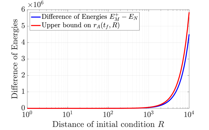
We fix $t_{f}=10$ and vary the distance $R$ of the initial condition $x_{0}$ from the origin. Figure 1(a) shows the difference between the worst-case total energy $\overline{E}_{M}$ and the nominal energy $E_{N}$ as a function of the distance $R$ of the initial condition $x_{0}$ from the origin. We also plot the upper bound on $r_{A}(t_{f},R)$ from (35) as a function of $R$ , and note that this is a useful upper bound characterizing the additional energy used by the malfunctioning system.

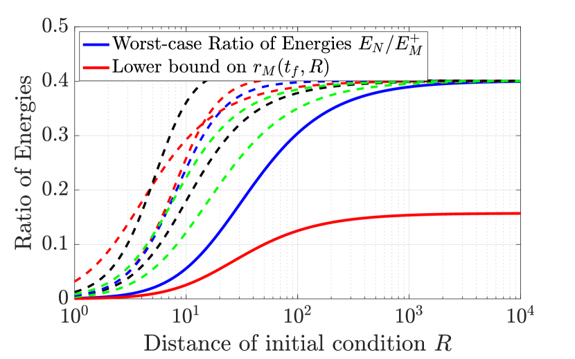
Similarly, Fig. 1(b) shows the ratio of the nominal energy $E_{N}$ and the total energy $E_{M}^{+}$ as a function of $R$ . Here, we test a large class of uncontrolled inputs, including constant, full-amplitude inputs of the form (32) and different classes of low- and high-frequency sinusoids. We also plot the lower bound on $r_{M}(t_{f},R)$ from (37) as a function of $R$ , shown in the thick red line. It is evident that $r_{M}(t_{f},R)$ bounds the ratio of nominal and augmented malfunctioning energies from below. Furthermore, the thick blue line represents the ratio $E_{N}/E_{M}^{+}$ for the worst-case uncontrolled input in (32), where $E_{M}^{+}=\overline{E}_{M}$ . The bound on $r_{M}(t_{f},R)$ is a reasonable approximation for this ratio, especially for initial conditions closer to the origin. For instance, when $R=10$ , we have $r_{M}(t_{f},R)\approx 0.03$ , while $E_{N}/\overline{E}_{M}\approx 0.05$ . The bound on $r_{M}(t_{f},R)$ indicates that at most $1/0.03=33.33$ times more energy is used by the actuators to achieve finite-time regulation when a loss of control authority of the form described above occurs. The actual ratio indicates that around $1/0.05\approx 20$ times the energy is required to achieve the task. The metric $r_{M}(t_{f},R)$ is thus a useful quantity to characterize the maximal additional energy required to achieve a task when control authority is lost over a subset of actuators.

If we considered the model used by [13], where the effect of $u_{1}$ on $x$ is weighted more, these metrics would be relatively less useful in characterizing the additional energy required, in comparison to the model in (39). The heavier weight contributes to poor conditioning of the matrices $B^{\dagger T}B^{\dagger}$ and $B_{c}^{\dagger T}B_{c}^{\dagger}$ , resulting in more conservative bounds in (35) and (37) than in the example presented here.

VI Conclusions and Future Work

In this paper, our objective was to quantify the maximal additional energy used by a system which loses control authority over a subset of actuators, compared to the nominal system with full control authority. To this end, we considered the special case of linear driftless systems and introduced additive and multiplicative energetic resilience metrics. These metrics compare the nominal and worst-case total energies to achieve finite-time regulation. Deriving the nominal and worst-case total energies for this task used a technical lemma proved using the calculus of variations. We also obtained the optimal final time that minimizes the malfunctioning energy for a given uncontrolled input. When considering the special case of losing control authority over one actuator, we obtained an exact expression for the worst-case total energy, allowing us to obtain bounds on the energetic resilience metrics. A simulation example on a model of an underwater robot demonstrated the applicability of these metrics in characterizing the additional energy used by a malfunctioning system.

Future work involves examining general linear and nonlinear systems. Obtaining energy-optimal control signals in these cases is not a straightforward task due to the input constraints $u\in\operatorname*{\mathcal{U}}$ and $u_{c}\in\operatorname*{\mathcal{U}_{c}}$ . Other complexities, such as systems with time delays and systems whose general structure is uncertain due to unmodeled dynamics, are also to be examined.

References

[1] M. Bartels, “Russia’s Nauka module briefly tilts space station with unplanned thruster fire,” Aug. 2021. [Online]. Available: https://www.space.com/nauka-module-thruster-fire-tilts-space-station
[2] B. Roberston and E. Stoneking, “Satellite GN&C anomaly trends,” in 26th Annual AAS Guidance and Control Conference, Breckenridge, CO, USA, Feb. 2003.
[3] Q. Hu, B. Li, B. Xiao, and Y. Zhang, Control Allocation for Spacecraft Under Actuator Faults. Singapore: Springer Nature, 2021.
[4] R. C. Suich and R. L. Patterson, “How much redundancy: Some cost considerations, including examples for spacecraft systems,” in AIChE Summer National Meeting Session on Space Power Systems Technology, San Diego, CA, USA, Aug. 1990.
[5] W. Grossman, “Autonomous control system reconfiguration for spacecraft with non-redundant actuators,” in Estimation Theory Symposium, Greenbelt, MD, USA, May 1995.
[6] A. Boche, J.-L. Farges, and H. Plinval, “Reconfiguration control method for non-redundant actuator faults on unmanned aerial vehicle,” Proceedings of the Institution of Mechanical Engineers, Part G: Journal of Aerospace Engineering, vol. 234, no. 10, pp. 1597–1610, Aug. 2019.
[7] G. Tao, S. Chen, and S. Joshi, “An adaptive actuator failure compensation controller using output feedback,” IEEE Transactions on Automatic Control, vol. 47, no. 3, pp. 506–511, Mar. 2002.
[8] B. Xiao, Q. Hu, and P. Shi, “Attitude stabilization of spacecrafts under actuator saturation and partial loss of control effectiveness,” IEEE Transactions on Control Systems Technology, vol. 21, no. 6, pp. 2251–2263, Nov. 2013.
[9] A. A. Amin and K. M. Hasan, “A review of fault tolerant control systems: Advancements and applications,” Measurement, vol. 143, pp. 58–68, Sept. 2019.
[10] J.-B. Bouvier and M. Ornik, “Designing resilient linear systems,” IEEE Transactions on Automatic Control, vol. 67, no. 9, pp. 4832–4837, Sep. 2022.
[11] L. Y. Wang and J.-F. Zhang, “Fundamental limitations and differences of robust and adaptive control,” in 2001 American Control Conference, Arlington, VA, USA, June 2001, pp. 4802–4807.
[12] B. D. O. Anderson and A. Dehghani, “Challenges of adaptive control–past, permanent and future,” Annual Reviews in Control, vol. 32, no. 2, pp. 123–135, Dec. 2008.
[13] J.-B. Bouvier and M. Ornik, “Resilient reachability for linear systems,” in 21st IFAC World Congress, Berlin, Germany, July 2020, pp. 4409–4414.
[14] J.-B. Bouvier, K. Xu, and M. Ornik, “Quantitative resilience of linear driftless systems,” in SIAM Conference on Control and its Applications, July 2021, pp. 32–39, (Virtual).
[15] J.-B. Bouvier and M. Ornik, “Quantitative resilience of linear systems,” in 2022 European Control Conference (ECC), London, United Kingdom, May 2022, pp. 485–490.
[16] ——, “Resilience of linear systems to partial loss of control authority,” Automatica, vol. 152, June 2023.
[17] R. Padmanabhan, C. Bakker, S. A. Dinkar, and M. Ornik, “How much reserve fuel: Quantifying the maximal energy cost of system disturbances,” in 63rd IEEE Conference on Decision and Control, Milan, Italy, Dec. 2024. [Online]. Available: https://arxiv.org/abs/2408.10913
[18] B. Siciliano and O. Khatib, Eds., Springer Handbook of Robotics. Heidelberg, Germany: Springer Berlin, 2008.
[19] J. Yu, C. Wang, and G. Xie, “Coordination of multiple robotic fish with applications to underwater robot competition,” IEEE Transactions on Industrial Electronics, vol. 63, no. 2, pp. 1280–1288, Feb. 2016.
[20] R. Penrose, “A generalized inverse for matrices,” Mathematical Proceedings of the Cambridge Philosophical Society, vol. 51, no. 3, pp. 406–413, July 1955.
[21] R. A. Horn and C. R. Johnson, Matrix Analysis, 2nd ed. New York, NY, USA: Cambridge University Press, 2013.
[22] R. E. Kalman and J. E. Bertram, “Control system analysis and design via the “second method” of Lyapunov: I—Continuous-time systems,” Journal of Basic Engineering, vol. 82, no. 2, pp. 371–393, June 1960.
[23] D. Liberzon, Calculus of Variations and Optimal Control Theory: A Concise Introduction. Princeton, NJ, USA: Princeton University Press, 2012.
[24] R. Penrose, “On best approximate solutions of linear matrix equations,” Mathematical Proceedings of the Cambridge Philosophical Society, vol. 52, no. 1, pp. 17–19, Jan. 1956.
[25] D. Bertsimas and J. N. Tsitsiklis, Introduction to Linear Optimization. Belmont, MA, USA: Athena Scientific, 1997.
[26] J.-B. Bouvier and M. Ornik, “The maximax minimax quotient theorem,” Journal of Optimization Theory and Applications, vol. 192, no. 3, pp. 1084–1101, Mar. 2022.

$\displaystyle r_{A}(t_{f},R)$	$\displaystyle=\sup_{\\|x_{0}\\|_{2}\leq R}\Biggl{\{}\frac{1}{t_{f}}\left\\|B_{c}^{\dagger}x_{0}\right\\|_{2}^{2}+t_{f}\left(\\|B_{uc}\\|_{2}^{2}+1\right)$
	$\displaystyle+2\left\|B_{uc}^{T}B_{c}^{\dagger T}B_{c}^{\dagger}x_{0}\right\|-\frac{1}{t_{f}}\left\\|B^{\dagger}x_{0}\right\\|_{2}^{2}\Biggr{\}}$
	$\displaystyle\leq t_{f}\left(\\|B_{uc}\\|_{2}^{2}+1\right)+2R\\|B_{uc}^{T}B_{c}^{\dagger T}B_{c}^{\dagger}\\|_{2}$
	$\displaystyle+\sup_{\\|x_{0}\\|_{2}\leq R}\frac{1}{t_{f}}x_{0}^{T}\left(B_{c}^{\dagger T}B_{c}^{\dagger}-B^{\dagger T}B^{\dagger}\right)x_{0},$	(36)