End-to-End Multi-channel Transformer for Speech Recognition

Like other sequence-to-sequence learning problems, we start by projecting the source channel features and one-hot token vector to the dense embedding spaces, for more discriminative representations. The $i^{th}$ channel feature matrix, $X_{i}$, contains magnitude features $X_{i}^{mag}$ and phase features $X_{i}^{pha}$; more details will be described in Sec. 3. We use three linear projection layers, $W^{me}_{i}$, $W^{pe}_{i}$, and $W^{je}_{i}$ to embed the magnitude, phase, and their concatenated embeddings, respectively. Since the transformer networks do not model the position of a token within a sequence, we employ the positional encoding (PE) [21] to add the temporal ordering into the embeddings. The overall embedding process can be formulated as:

$\displaystyle\hat{X_{i}}=[X_{i}^{mag}W^{me}_{i},X_{i}^{pha}W^{pe}_{i}]W^{je}_{i}+\textbf{PE}(t,f)$

(1)

Here, all the bias vectors are ignored and $[.,.]$ indicates the concatenation. $\hat{X_{i}}\in\mathbb{R}^{T\times d_{m}}$, where $d_{m}$ is the embedding size. $i\in\{1,...,C\}$, $t\in\{1,...,T\}$, and $f\in\{1,...,d_{m}\}$. Similarly, the token embedding is formulated as:

$\displaystyle\hat{\textbf{y}}_{j}=W^{te}\textbf{y}_{j}+\textbf{b}^{te}+\textbf{PE}(j,l)$

(2)

Here $W^{te}$ and $\textbf{b}^{te}$ are learnable token-specific weight and bias parameters. $\hat{\textbf{y}}_{j}\in\mathbb{R}^{d_{m}\times 1}$, $j\in\{1,...,U\}$, and $l\in\{1,...,d_{m}\}$.

Channel-wise Self Attention Layer (CSA): Each encoder layer starts from utilizing self-attention layers per channel (Fig. 2(b)) in order to learn the contextual relationship within a single channel. Following [21], we use the multi-head scaled dot-product attention (MH-SDPA) as the scoring function shown in Fig. 2(a) to compute the attention weights across time. Given the $i^{th}$ channel embeddings, $\hat{X}_{i}$, by Eq.(1), we can obtain the queries, keys, and values via the linear transformations followed by an activation function as:

	$\displaystyle Q^{cs}_{i}=\sigma\left(\hat{X}_{i}W^{cs,q}+\textbf{1}(\textbf{b}^{cs,q}_{i})^{T}\right)$
	$\displaystyle K^{cs}_{i}=\sigma\left(\hat{X}_{i}W^{cs,k}+\textbf{1}(\textbf{b}^{cs,k}_{i})^{T}\right)$		(3)
	$\displaystyle V^{cs}_{i}=\sigma\left(\hat{X}_{i}W^{cs,v}+\textbf{1}(\textbf{b}^{cs,v}_{i})^{T}\right)$

Here $\sigma(.)$ is the $ReLU$ activation function, $W^{cs,*}\in\mathbb{R}^{d_{m}\times d_{m}}$ and $\textbf{b}^{cs,*}\in\mathbb{R}^{d_{m}\times 1}$ are learnable weight and bias parameters, and $\textbf{1}\in\mathbb{R}^{T\times 1}$ is an all-ones vector. The channel-wise self attention output is then computed by:

$\displaystyle H^{cs}_{i}=Softmax\left(\frac{Q^{cs}_{i}(K^{cs}_{i})^{T}}{\sqrt{d_{m}}}\right)V^{cs}_{i}$

(4)

where the scaling $\frac{1}{\sqrt{d_{m}}}$ is for numerical stability [21]. We then add the residual connection [30] and layernorm [29] (See Fig. 2(b)) before feeding the contextual time-attended representations through the feed forward layers in order to get final channel-wise attention outputs $\hat{H^{cs}_{i}}$, as shown on the top of Fig. 2(b).

Cross-channel Attention Layer (CCA): The cross-channel attention layer (Fig. 2(c)) learns not only the cross correlation in time between time frames but also cross correlation between channels given the self-attended channel representations, $\{\hat{H}^{cs}_{i}\}^{C}_{i=1}$. We propose to create $Q$, $K$ and $V$ as follows:

	$\displaystyle Q^{cc}_{i}=\sigma\left(\hat{H}^{cs}_{i}W^{cc,q}+\textbf{1}(\textbf{b}^{cc,q}_{i})^{T}\right)$
	$\displaystyle K^{cc}_{i}=\sigma\left(H^{CCA}W^{cc,k}+\textbf{1}(\textbf{b}^{cc,k}_{i})^{T}\right)$		(5)
	$\displaystyle V^{cc}_{i}=\sigma\left(H^{CCA}W^{cc,v}+\textbf{1}(\textbf{b}^{cc,v}_{i})^{T}\right)$

$\displaystyle H^{CCA}=\sum_{j,j\neq i}A_{j}\odot\hat{H}^{cs}_{j}$

(6)

where $\hat{H}^{cs}_{i}$ is the input for generating the queries. In addition, the keys and values are generated by the weighted-sum of contributions from the other channels, $\{\hat{H}^{cs}_{j}\}^{C}_{j=1,j\neq i}$, i.e. Eq. (6), which is similar to the beamforming process. Note that $A_{j}$, $W^{cc,*}$ and $\textbf{b}^{cc,*}$ are learnable weight and bias parameters, and $\odot$ indicates element-wise multiplication. The cross-channel attention output is then computed by:

$\displaystyle H^{cc}_{i}=Softmax\left(\frac{Q^{cc}_{i}(K^{cc}_{i})^{T}}{\sqrt{d_{m}}}\right)V^{cc}_{i}$

(7)

To the best of our knowledge, it is the first time this cross channel attention mechanism is introduced within the transformer network for multi-channel ASR.

Similar to CSA, we feed the contextual channel-attended representations through feed forward layers to get the final cross-channel attention outputs, $\hat{H^{cc}_{i}}$, as shown on the top of Fig. 2(c). To learn more sophisticated contextual representations, we stack multiple CSAs and CCAs to from the encoder network output $\{H^{e}_{i}\}^{C}_{i=1}$ in Fig. 2(d).

Multi-channel encoder-decoder attention (EDA): Similar to [21], we employ the masked self-attention layer (MSA), $\hat{H^{sa}}$, to model the contextual relationship between target tokens and their predecessors. It is computed similarly as in Eq. (3) and (4) but with token embeddings (Eq. 2) as inputs. Then we create the queries by $\hat{H^{sa}}$, and keys as well as values by the multi-channel encoder outputs $\{H^{e}_{i}\}^{C}_{i=1}$ as follows:

	$\displaystyle Q^{ed}=\sigma\left(\hat{H^{sa}}W^{ed,q}+\textbf{1}(\textbf{b}^{md,q})^{T}\right)$
	$\displaystyle K^{ed}=\sigma\left(\frac{1}{C}\sum^{C}_{i=1}H^{e}_{i}W^{ed,k}+\textbf{1}(\textbf{b}^{md,k})^{T}\right)$		(8)
	$\displaystyle V^{ed}=\sigma\left(\frac{1}{C}\sum^{C}_{i=1}H^{e}_{i}W^{ed,v}+\textbf{1}(\textbf{b}^{ed,v})^{T}\right)$

Again, $W^{ed,*}$ and $\textbf{b}^{ed,*}$ are learnable weight and bias parameters. The multi-channel decoder attention then becomes the regular encoder-decoder attention of the transformer decoder. Similarly, by applying MH-SDPA, layernorm, and feed forward layer, we can get final decoder output, $\hat{H^{ed}}$, as shown on the top of Fig. 2(d). To train our multi-channel transformer, we use the cross-entropy loss with label smoothing of value $\epsilon_{ls}=0.1$ [31].

To evaluate our multi-channel transformer method (MCT), we conduct a series of ASR experiments using over 2,000 hours of speech utterances from our in-house anonymized far-field dataset. The amount of training set, validation set (for model hyper-parameter selection), and test set are 2,000 hours (312,0000 utterances), 4 hours (6,000 utterances), and 16 hours (2,5000 utterances) respectively. The device-directed speech data was captured using smart speaker with 7 microphones, and the aperture is 63mm. The users may move while speaking to the device so the interaction with the devices were completely unconstrained. In this dataset, 2 microphone signals of aperture distance and the super-directive beamformed signal by [11] using 7 microphone signals are employed through all the experiments.

We compare our multi-channel transformer (MCT) to four baselines: (1) Single channel + Transformer (SCT): This serves as the single-channel baseline. We feed each of two raw channels individually into the transformer for training and testing, and obtain the average WER from the two channels. (2) Super-directive (SD) beamformer [11] + Transformer (SDBF-T): The SD BF is widely used in the speech-directed devices including the one we used to obtain the beamformed signal in the in-house dataset. This beamformer used all seven microphones for beamforming. Multiple beamformers are built on the frequency domain toward different look directions and one with the maximum energy is selected for the ASR input; therefore, the input features to the transformer are extracted from a single channel of beamformed audio. (3) Neural beamformer [10] + Transformer (NBF-T): This serves as the fixed beamformer (FBF) baseline using two microphone signals as inputs rather than seven in SD beamformer. Multiple beamforming matrices toward seven beam directions followed by a convolutional layer are learned to combine multiple channels, and then the energy features from all beam directions respectively. The beamforming matrices are initialized with MVDR beamformer [20]. (4) Neural masked-based beamformer [13] + Transformer (NMBF-T): It serves as the adaptive beamforming (ABF) baseline, and also uses two microphone signals as inputs. The mask estimator was pre-trained following [13]. Note that the above neural beamforming models are jointly finetuned with the transformers.

The transformers in all the baselines and our multi-channel transformer (MCT) are of $d_{m}=256$, number of hidden neurons $d_{ff}=1,024$, and number of heads, $h=3$. While MCT and the transformer for NMBF-T have $N_{e}=4$ and $N_{d}=4$, other transformers are of $N_{e}=6$, $N_{d}=6$ in order to have comparable model size, as shown in Table 1. Note that NMBF-T is about 5M larger than the other methods due to the BLSTM and FeedForward layers used in the mask estimator of [13]. Results of all the experiments are demonstrated as the relative word error rate reduction (WERR). Given a method A’s WER ($\text{WER}_{A}$) and a baseline B’s WER ($\text{WER}_{B}$), the WERR of A over B can be computed by $(\text{WER}_{B}-\text{WER}_{A})/\text{WER}_{B}$; the higher the WERR is the better.

The input features, the Log-STFT square magnitude (for SCT and SDBF-T) and STFT (for NBF-T and NMBF-T) are extracted every 10 ms with a window size of 25 ms from 80K audio samples (results in $T=166$ frames per utterance); the features of each frame is then stacked with the ones of left two frames, followed by downsampling of factor 3 to achieve low frame rate, resulting in $F=768$ feature dimensions. In the proposed method, we use both log-STFT square magnitude features, and phase features following [32, 33] by applying the sine and cosine functions upon the principal angles of the STFT at each time-frequency bin. We used the Adam optimizer [34] and varied the learning rate following [21, 22] for optimization. The subword tokenizer [35] is used to create tokens from the transcriptions; we use $L=4,002$ tokens in total.

Table 1 shows the performances of our method (MCT-2) and beamformers+transformers methods over different baselines. While all cascaded beamformers+transformers methods perform better than SCT (by 2.07% to 6%), our method improves the WER the most (by 11.21%). When comparing WERRs over SDBF-T, however, only MCT-2 improves the WER. The degradations from NBF-T and NMBF-T over SDBF-T may be attributed to not only 2 rather than 7 microphones are used but also the suboptimal front-end formalizations either by using a fixed set of weights for look direction fusion (NBF-T) or flawed speech/noise mask estimations (NMBF-T). If we compare our method directly to NBF-T and NMBF-T, we see 9% and 9.33% relative improvements respectively. We further investigate whether the information from the super-directive beamformer channel was complementary to the multi-channel transformer. To this end, we take the beamformed signal from SD beamformer as the third channel and feed it together with the other two channels to our transformer (MCT-3). We see in Table 1 (the last row), about 10% extra relative improvements are achieved compared to MCT-2.

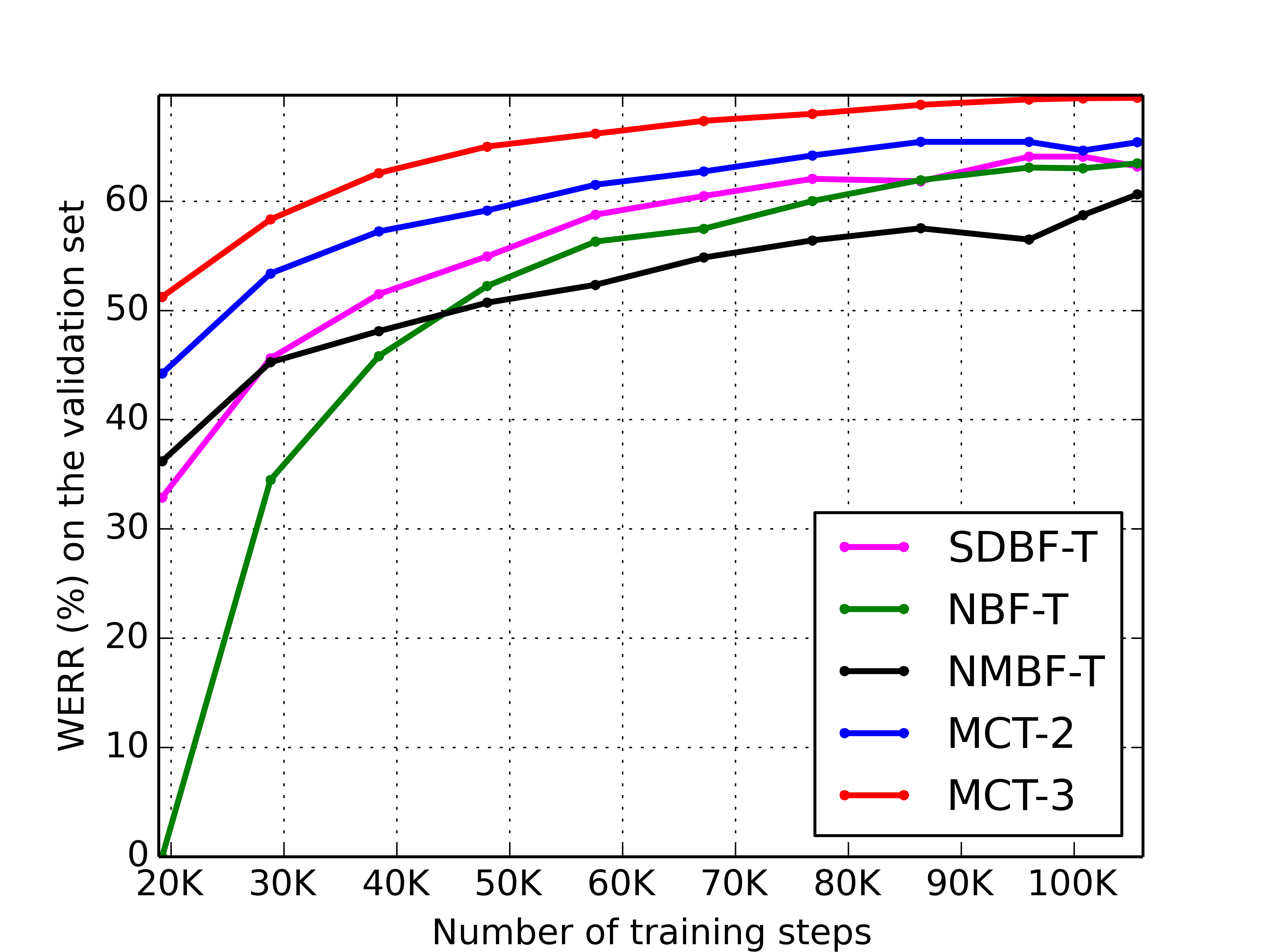
In Fig. 3, we evaluate the convergence rate and quality via comparing the learning curves of our model to the other beamformer-transformer cascaded methods. Note that our model has started to converge at around 100K training steps, while the others have not. We compute the WERRs of all methods over a fixed reference point, which is the highest WER point during this period by NBF-T (the left-most point of NBF-T corresponding to WERR=0). Our method converges faster than the others with consistently higher relative WER improvements. Also, we observe NMBF-T converges the slowest, and the NBF-T is the second slowest.

Finally, we conducted an ablation study to demonstrate the importance of channel-wise self attention (CSA) and cross-channel attention (CCA) layers. To this end, we train two variants of multi-channel transformers by using CSA only or CCA only. Table 2 shows that the WERR drops significantly when either attention is removed.

Furthermore, our model can be simply applied on more than 3 channels. In an 8-microphone case, the number of parameters would increase by only about 10% ($T\times d_{m}\times N_{e}\times 8/10^{6}/13.3=166\times 256\times 4\times 8/10^{6}/13.3$) compared to the one-microphone case ($13.3$M parameters).

References

- [1] Maurizio Omologo, Marco Matassoni, and Piergiorgio Svaizer, “Speech recognition with microphone arrays,” in Microphone arrays, pp. 331–353. Springer, 2001.
- [2] Matthias Wölfel and John McDonough, Distant speech recognition, John Wiley & Sons, 2009.
- [3] Kenichi Kumatani, John McDonough, and Bhiksha Raj, “Microphone array processing for distant speech recognition: From close-talking microphones to far-field sensors,” IEEE Signal Processing Magazine, vol. 29, no. 6, pp. 127–140, 2012.
- [4] Keisuke et al. Kinoshita, “A summary of the reverb challenge: state-of-the-art and remaining challenges in reverberant speech processing research,” EURASIP Journal on Advances in Signal Processing, vol. 2016, no. 1, pp. 7, 2016.
- [5] Tuomas Virtanen, Rita Singh, and Bhiksha Raj, Techniques for noise robustness in automatic speech recognition, John Wiley & Sons, 2012.
- [6] Tobias Menne, Jahn Heymann, Anastasios Alexandridis, Kazuki Irie, Albert Zeyer, Markus Kitza, Pavel Golik, Ilia Kulikov, Lukas Drude, Ralf Schlüter, Hermann Ney, Reinhold Haeb-Umbach, and Athanasios Mouchtaris, “The rwth/upb/forth system combination for the 4th chime challenge evaluation,” in CHiME-4 workshop, 2016.
- [7] Jon Barker, Ricard Marxer, and et al., “The third ‘chime’speech separation and recognition challenge: Dataset, task and baselines,” in ASRU, 2015.
- [8] Xuankai Chang, Wangyou Zhang, Yanmin Qian, Jonathan Le Roux, and Shinji Watanabe, “Mimo-speech: End-to-end multi-channel multi-speaker speech recognition,” in ASRU, 2019.
- [9] Xuankai Chang, Wangyou Zhang, Yanmin Qian, Jonathan Le Roux, and Shinji Watanabe, “End-to-end multi-speaker speech recognition with transformer,” in ICASSP, 2020.
- [10] Kenichi Kumatani, Wu Minhua, Shiva Sundaram, Nikko Ström, and Björn Hoffmeister, “Multi-geometry spatial acoustic modeling for distant speech recognition,” in ICASSP, 2019.
- [11] Simon Doclo and Marc Moonen, “Superdirective beamforming robust against microphone mismatch,” IEEE Transactions on Audio, Speech, and Language Processing, vol. 15, no. 2, pp. 617–631, 2007.
- [12] Ivan Himawan, Iain McCowan, and Sridha Sridharan, “Clustered blind beamforming from ad-hoc microphone arrays,” TASLP, vol. 19, no. 4, pp. 661–676, 2010.
- [13] Jahn Heymann, Lukas Drude, and Reinhold Haeb-Umbach, “Neural network based spectral mask estimation for acoustic beamforming,” in ICASSP, 2016.
- [14] Hakan Erdogan, John R Hershey, and et al., “Improved mvdr beamforming using single-channel mask prediction networks.,” in Interspeech, 2016.
- [15] Tsubasa Ochiai, Shinji Watanabe, and et al., “Multichannel end-to-end speech recognition,” arXiv preprint arXiv:1703.04783, 2017.
- [16] Wu Minhua, Kenichi Kumatani, Shiva Sundaram, Nikko Ström, and Björn Hoffmeister, “Frequency domain multi-channel acoustic modeling for distant speech recognition,” in ICASSP, 2019.
- [17] Bo Li, Tara N Sainath, and et al., “Neural network adaptive beamforming for robust multichannel speech recognition,” in Interspeech, 2016.
- [18] Xiong Xiao, Shinji Watanabe, and et al., “Deep beamforming networks for multi-channel speech recognition,” in ICASSP, 2016.
- [19] Zhong Meng, Shinji Watanabe, and et al., “Deep long short-term memory adaptive beamforming networks for multichannel robust speech recognition,” in ICASSP, 2017.
- [20] Jack Capon, “High-resolution frequency-wavenumber spectrum analysis,” Proceedings of the IEEE, vol. 57, no. 8, pp. 1408–1418, 1969.
- [21] Ashish Vaswani, Noam Shazeer, Niki Parmar, Jakob Uszkoreit, Llion Jones, Aidan N Gomez, Lukasz Kaiser, and Illia Polosukhin, “Attention is all you need,” in NeurNIPS, 2017.
- [22] Linhao Dong, Shuang Xu, and Bo Xu, “Speech-transformer: a no-recurrence sequence-to-sequence model for speech recognition,” in ICASSP, 2018.
- [23] Liang Lu, Changliang Liu, Jinyu Li, and Yifan Gong, “Exploring transformers for large-scale speech recognition,” arXiv preprint arXiv:2005.09684, 2020.
- [24] Yongqiang et al. Wang, “Transformer-based acoustic modeling for hybrid speech recognition,” in ICASSP, 2020.
- [25] Martin Radfar, Athanasios Mouchtaris, and Siegfried Kunzmann, “End-to-end neural transformer based spoken language understanding,” in Interspeech, 2020.
- [26] Georgios Paraskevopoulos, Srinivas Parthasarathy, Aparna Khare, and Shiva Sundaram, “Multiresolution and multimodal speech recognition with transformers,” arXiv preprint arXiv:2004.14840, 2020.
- [27] Bahareh Tolooshams, Ritwik Giri, Andrew H Song, Umut Isik, and Arvindh Krishnaswamy, “Channel-attention dense u-net for multichannel speech enhancement,” in ICASSP, 2020.
- [28] Lukas Drude, Jahn Heymann, and Reinhold Haeb-Umbach, “Unsupervised training of neural mask-based beamforming,” arXiv preprint arXiv:1904.01578, 2019.
- [29] Jimmy Lei Ba, Jamie Ryan Kiros, and Geoffrey E Hinton, “Layer normalization,” arXiv preprint arXiv:1607.06450, 2016.
- [30] Kaiming He, Xiangyu Zhang, Shaoqing Ren, and Jian Sun, “Deep residual learning for image recognition,” in CVPR, 2016.
- [31] Christian Szegedy and Vincent et al. Vanhoucke, “Rethinking the inception architecture for computer vision,” in CVPR, 2016.
- [32] Zhong-Qiu Wang and DeLiang Wang, “Combining spectral and spatial features for deep learning based blind speaker separation,” TASLP, vol. 27, no. 2, pp. 457–468, 2018.
- [33] Zhong-Qiu Wang, Jonathan Le Roux, and John R Hershey, “Multi-channel deep clustering: Discriminative spectral and spatial embeddings for speaker-independent speech separation,” in ICASSP, 2018.
- [34] Diederik P Kingma and Jimmy Ba, “Adam: A method for stochastic optimization,” arXiv preprint arXiv:1412.6980, 2014.
- [35] Rico Sennrich, Barry Haddow, and Alexandra Birch, “Neural machine translation of rare words with subword units,” in ACL, 2016.