Encoding Binary Concepts in the Latent Space of Generative Models for Enhancing Data Representation
Abstract
Binary concepts111“Concepts” are also known as “factors” in unsupervised learning literature. We use these terms interchangeably. are empirically used by humans to generalize efficiently. And they are based on Bernoulli distribution which is the building block of information. These concepts span both low-level and high-level features such as “large vs small” and “a neuron is active or inactive”. Binary concepts are ubiquitous features and can be used to transfer knowledge to improve model generalization. We propose a novel binarized regularization to facilitate learning of binary concepts to improve the quality of data generation in autoencoders. We introduce a binarizing hyperparameter in data generation process to disentangle the latent space symmetrically. We demonstrate that this method can be applied easily to existing variational autoencoder (VAE) variants to encourage symmetric disentanglement, improve reconstruction quality, and prevent posterior collapse without computation overhead. We also demonstrate that this method can boost existing models to learn more transferable representations and generate more representative samples for the input distribution which can alleviate catastrophic forgetting using generative replay under continual learning settings.
1 Introduction
There is a famous game named Akinator. It asks you a series of binary answer questions such as “is he young or old?” or “is she an actress” to find out what subject you are thinking of based on your answers. A recent study [24] suggests humans use a similar strategy to ask questions with binary answers to maximize information gain. This implies that humans use binary concepts to efficiently encode information internally to discriminate between concepts. In reinforcement learning, there is evidence [26] that an agent can generalize low-level physical properties by sequentially binarizing observations. The above evidence serves as an inspiration to benefit from binarized concepts to learn latent space representations for an input distribution such that they disentangle concepts in a binary scheme to potentially facilitate learning all factors. We especially apply our approach on VAEs since they learn stable latent representations.

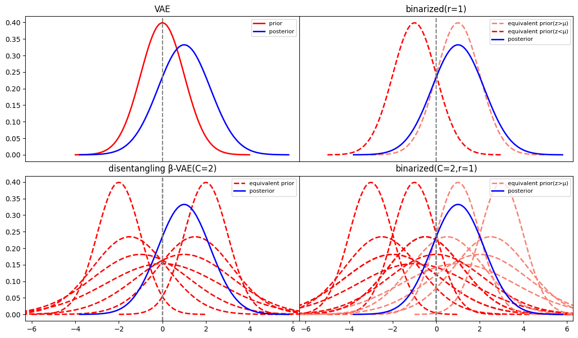
Most existing variants of VAEs focus on regularizing the latent space to learn more disentangled factors to boost efficiency and the quality of generated data. Considering that (i) low-level information-dense factors are difficult to disentangle, and are often treated as noise (posterior collapse) and (ii) high-level information-scarce factors are easy to disentangle, they usually lead to learning low-variance representations. As a result, generated samples are highly biased toward the mean of the learned distribution in the latent space and hence are less diverse compared to the real-world data. To our knowledge, existing methods are not exploring the possibility of learning an inherent property shared by all levels of factors in real-world data. We argue that binary concepts in the latent representation are a suitable candidate for this purpose (see Figure 1).
We introduce a general regularization technique to improve VAEs. We call it “binarized” regularization because it enforces learning latent distributions that approximate the posterior using two symmetric modalities in each dimension of the latent space (see Figure 1). As a result, the latent distribution mass deterministically moves towards one of the closest prior distributions on a high-dimensional grid of a mixture distribution that allows generating diverse samples (note Figure 1 is an example for a 2D latent embedding space). We demonstrate that our regularization technique improves disentanglement of the latent and simultaneously improves reconstruction quality through extensive experiments. Our specific contributions include:
-
•
We develop a regularization technique to binarize the VAE objective and demonstrate that binarized VAEs are able to further disentangle the latent, resolve noisy low-level factors in generated images, and can generate significantly more variant high-level features.
-
•
We demonstrated that our method can prevent posterior collapsing by restoring the collapsed latent representation to learn low-level factors.
-
•
We further adopt our idea to address catastrophic forgetting in continual learning. Results demonstrate that our method is able to generate more diverse samples for the past tasks and compares favorably against state-of-the-art generative replay methods on the most challenging incremental-class classification tasks.
2 Background and Related Work
Variational Autoencoders
have an extremely rich literature. We propose a unified framework to formulate all current VAE-based methods in Figure 2. We argue that a Gaussian Mixture Model (GMM) can be used to model any complicatedly-distributed latent concepts using a combination of an infinite number of simply-distributed high-level to low-level concepts. These concepts continuously span from high-variance to low-variance. The gaps in Figure 2 represent how close the distributions are between Gap 1: prior and true posterior222the optimal mapping from data to a regularized distribution, Gap 2 (L/R): approximate posterior and true posterior, and Gap 3 (L/R): approximate posterior and prior. A smaller Gap 2 leads to a better reconstruction quality. A smaller Gap 3 leads to better disentanglement. The goal of the VAE optimizations can be generalized as reducing Gap 3 (preferably without reducing Gap 2). Within this formulation, the prominent VAE variants can be categorized by the way they achieve this goal:
(i) Reducing the size of Gap 1: These methods indirectly reduce both Gaps 2 and 3 on certain types of true posteriors. Gaussian VAE [12] uses a unimodal Gaussian distribution as the prior. It can serve as a good approximation for many true posteriors but the generated samples are biased towards its mean and may not be very diverse. Hyperspherical VAE (NVAE) [5] uses von Mises-Fisher (vMF) prior that is closer to some specific true posteriors.
(ii) Reducing the size of Gap 3 by trading-off the size of Gap 2: -VAE [8] uses a hyperparameter to do so.
(iii) Reducing the size of Gap 3 with adaptable priors: GMVAE [6] creates a finite set of candidate priors. disentangling -VAE[2] creates an infinite set of candidate priors on an “equal KL-divergence” line (see Figure 3 row 2 column 1 all dashed curves for clarity).
(iv) Reducing the size of Gap 3 by adapting the prior to approximate the posterior: VAMP [27] has a mixture prior, and uses aggregate posterior333The observed latent distribution on aggregate seen data. to move prior towards the approximated posterior during training. -TCVAE [3] adds a regularization term to optimize the prior towards the posterior during training. DIP-VAE [15] uses the concept of “moment” to predict the future posterior, and uses this extra information to move the prior towards the approximate posterior. FactorVAE [11] adds a regularization term to factorize prior to adapt to low-variance posterior.

(v) Reducing the size of Gap 2R and Gap 3R with a low-variance local prior: To achieve this goal without increasing Gap 2L and 3L, having many low-variance approximate posteriors is necessary to approximate the high-variance distribution. These posteriors result in an inaccurate approximation of hte high-level factors when a model is small. The extreme case is Autoencoders [22]. WAE [14] only maintains prior-like global approximate posteriors, but reduces the variance of local posteriors. VQVAE [16] nears the extreme with a no-variance quantized latent prior.
(vi) Reducing the size of Gap 2 and Gap 3 with larger models: A larger model can reduce Gap 2 and Gap 3 by providing an approximate posterior with a larger variance range. VDVAE[4] is an example in this category.
(vii) Reducing the size of Gap 2 with a less regularized likelihood prior: This approach is not within the VAE literature since it does not reduce Gap 3, but it is worth mentioning it due to its compatibility with this framework. The reconstruction prior used in VAEs is local low-variance Bournourli distribution. This requirement can be relaxed to more global distributions seen in GAN [7], or distributed throughout the full model as in diffusion models [9].
Our method employs ideas of (i) and (iii). When used on a unimodal Gaussian VAE, it is a GMVAE with components, with deterministic assignment conditioned on the approximate posterior, and unimodal Gaussian reparameterization to distributed the mass in the latent embedding.
Continual Learning
aims to learn a set of sequentially arriving tasks using a shared model. When the model is updated to learn the current task, we observe catastrophic forgetting [13] in the model due to deviation from the optimal parameters for the past learned tasks. CL algorithms employ three primary strategies to mitigate catastrophic forgetting. One approach involves regularizing a fixed shared model, such that different information pathways are used to learn each task’s weights [13, 1, 10]. The aim is to identify critical model parameters that encode the learned knowledge of each task and consolidate these parameters while updating the model to learn new tasks. The downside is that the learning capacity of the model is compromised as more weights are consolidated. Another approach relies on model expansion [23, 28], which involves adding new weights to a base model and customizing the network to learn new tasks via these additional weights. The downside is that the model can grow unboundedly as more tasks are learned. Finally, most algorithms employ pseudo-rehearsal through experience replay [17, 21, 18]. This method involves storing a representative subset of training data for each task in a memory buffer and replaying those samples along with the current task’s data to maintain encoded knowledge about previously learned. A group of algorithms relaxes the need for a memory buffer by building a generative model that learns to generate pseudo-samples that are very similar to the real samples of the past learned tasks. We demonstrate that our approach helps to improve this category of CL methods.
3 Problem Description
3.1 Variational Autoencoders Objective
Given a dataset , VAEs learn an encoder and a decoder that maximize the likelihood to approximate the empirical evidence . The encoder maps to a simple latent prior which has better sampling properties. The objective is to maximize:
where the right hand side is ELBO, served as the proxy objective we maximize to learn the latent distribution or as the objective in the following minimization problem:
| (1) |
where the first term is the negative likelihood of data after passing through the model. It is modeled as the reconstruction loss in VAEs. The second term is the KL-divergence between the approximate posterior and the latent prior.
3.2 Shortcoming of VAEs
The two terms in Eq. (1) conflict with each other. The first term trades disentanglement for reconstruction quality, emphasizing it results in low interpretability and control of latent representation. The second term trades reconstruction quality for disentanglement, emphasizing that it results in low variances of high-level concepts that lead to a high correlation with latent dimensions and high noise levels of low-level concepts that lead to posterior collapse. We develop a method to to mitigate these challenges.
4 Proposed Solution
4.1 Binarized Modification
We define a new binarized objective that instead of minimizing the distributional distance between the approximate posterior and the prior minimizes the closest distributional distance between the approximate posterior and two binarized priors which are located away from the mean of the prior. The new binarized loss can be written as:
| (2) | ||||
where is a model hyperparameter. It decides how disentangled the two candidate distributions are (see Figure 1). Note that the loss reduces to the original VAE loss when . A more general form can be written as:
| (3) |
for any loss function , where is a location variable of a prior distribution, and is a location variable of an approximate posterior distribution.
4.2 Binarized Gaussian Prior
Gaussian Prior Closed-form Loss
To add the binarized modification to a unimodal Gaussian prior , we have the closed form:
| (4) | ||||
We can show that this is equivalent to ELBO with a binarized -dependent prior as the following:
| (5) |
This equivalent prior can be visualized as in Figure 3. For more details on derivation please refer to the Appendix.
4.3 Reparametrization
We still use the original reparametrization trick since we still consider the original prior once the estimated posterior is decided. This assumption maintains the continuous property of the approximate posterior at the prior mean which is broken by the deterministic assignment. The probabilistic reparametrization and the deterministic assignment create an instability close to the prior mean, which can alleviate posterior collapse. The source of the instability is the opposing force provided by the Bernoulli-distribution-like encoding. It will have maximum information capacity when posterior collapse happens which discourages collapse.
4.4 Sampling
The instability at the prior mean will force the latent to deviate from the high probability density center. This allows more samples from the underrepresented outer region of high-variance factors, and fewer samples from the biased center high-density region, achieving reduced-bias sampling. Although this will negatively impact low-variance factors, in practice, the combined effect achieves better total sampling quality. This might be due to the alleviated posterior collapse compensating for this negative impact.


Reduced-bias Sampling: For the two binarized distributions, we assign an equal probability to sample from:
which is approximately sampling from the Gaussian:
when is small. In all of our experiments, this sampling method is used due to its simplicity and nice properties.
Biased Sampling: If we want to sample from the distribution when the input dataset is imbalanced, we restore the distribution of the dataset by conditioning the sampling prior on the latent statistics of the full dataset:
This sampling would for a skewed distribution.
5 Empirical Results
Experimental set-up: we used four types of VAE models: toyVAE is a feed-forward VAE, used to test theories and conduct ablation tests on the MNIST dataset. ConvVAE is a medium-size convolutional VAE, used for analytical experiments on MNIST and CelebA(32x32, 64x64) datasets. L-ConvVAE is a large-size convolutional VAE, used for qualitative visualization experiments on CelebA( 64x64) dataset. Cl-VAE is used for continual learning on splitMNIST, permutedMnist, and CIFAR100 datasets. All comparisons have identical model architecture, training settings, and data preprocessing. For details and implementation, refer to supplementary material.
5.1 Reconstruction and Unsupervised Clustering
First, we use toyVAE as the base model to compare the performance of binarized VAE with VAE on the MNIST dataset. Reconstruction is evaluated using image-sum pixel-wise binary cross-entropy (BCE). Unsupervised clustering is evaluated by normalized mutual information (NMI). The result is presented in Table 1. We observe that binarized VAE is able to achieve better reconstruction and clustering performances with different latent emebdding sizes.
| BCE | NMI | training time(s) | ||||||||||
|---|---|---|---|---|---|---|---|---|---|---|---|---|
| epochs | d | AE | VAE | NVAE | BVAE | AE | VAE | NVAE | BVAE | VAE | NVAE | BVAE |
| 10 | 2 | 136.19 | 138.72 | 136.83 | 135.66* | 0.546* | 0.505 | 0.535 | 0.536 | 10 | 13 | 10 |
| 4 | 111.84* | 114.01 | 114.33 | 112.83 | 0.675 | 0.657 | 0.647 | 0.695* | 10 | 17 | 10 | |
| 8 | 87.59 | 91.91 | 92.29 | 86.32* | 0.700 | 0.701 | 0.696 | 0.713* | 11 | 20 | 11 | |
| 16 | 69.23 | 85.46 | 81.52 | 67.85* | 0.691 | 0.700 | 0.671 | 0.746* | 14 | 24 | 14 | |
| 32 | 57.26 | 84.26 | 97.37 | 56.15* | 0.624 | 0.715* | 0.608 | 0.668 | 18 | 29 | 18 | |
| 20 | 2 | 134.03 | 135.43 | 132.91* | 134.32 | 0.530 | 0.565 | 0.578* | 0.556 | |||
| 4 | 109.36* | 112.05 | 110.61 | 109.81 | 0.691 | 0.670 | 0.677 | 0.712* | ||||
| 8 | 84.32 | 88.85 | 88.65 | 84.00* | 0.731 | 0.738 | 0.719 | 0.746* | ||||
| 16 | 65.63 | 83.27 | 76.70 | 64.87* | 0.749 | 0.695 | 0.740 | 0.754* | ||||
| 32 | 50.15* | 81.25 | 86.2 | 50.40 | 0.650 | 0.700* | 0.631 | 0.668 | ||||
Next, we scale the model to ConvVAE. We test VAE, -VAE, disentangling -VAE, and their binarized modifications (6 models) on the CelebA dataset (32x32 face-aligned). We again observe that the binarized models showed lower reconstruction loss (Figures 4 and 5), lower variational loss, and higher ELBO compared to the base models.
5.2 Analyzing Reconstruction and Sampling
We then further scale up the base model to L-ConvVAE. We test VAE, -VAE, disentangling -VAE, DIP-VAE, WAE and their binarized modifications on the CelebA (64x64 face-aligned) dataset, and visualize the reconstruction and sampling results in Figure 6. We use the same sampling latent space between the original and binarized models.

For reconstruction, the binarized versions have sharper edges and more detailed facial features in general and are more accurate in reconstructing those underrepresented categories in CelebA dataset such as old, facial hair, wearing a cap, etc. (Figure 7).

For sampling, we observe that low-level properties are similar between the samples, while high-level properties are well-distinctive and more variant in their binarized versions. This observation aligns well with our hypothesis. An interesting observation is that when binarizing WAE, the binarized model is able to generate samples with significantly more realistic facial features.
5.3 Resolving Posterior Collapsing
We use ConvVAE as the base model to visualize the latent space for MNIST and CelebA(32x32, 64x64 face-aligned) reduced-size(60000 instances) datasets. We tested VAE, -VAE, disentangling -VAE, and the binarized models. All the base models suffer from posterior collapse due to the adjusted smaller dataset compared to the large capacity of the ConvVAE decoder. We see that the binarized models are able to maintain the collapsed latent dimensions (see Figures 8 and 10), by introducing instability at the prior mean. concept (see Figure 8).

Then we look at what exact concepts are learned in the high-variance and low-variance latent dimensions. We see more variations of low-level binary concepts are learned by the binarized models in the high-variance dimensions (see Figure 9).

While high-level concepts are learned in the low-variance dimensions restored by the binarized models. While these concepts are unlearnable by the original VAE models (see Figure 10).

5.4 Generative Replay in Continual Learning
Generative replay requires the fit-sample-replay loop [25, 20, 19], which highly depends on the generated quality of the samples. First, we tested the compatibility of the Gaussian mixture prior to binarized regularization, since it is commonly used for conditional replay and proves to be effective. We test a GMVAE with a binarized GMVAE on MNIST (see Figure 11). We have compared state-of-the-art CL methods that use generative replay to mitigate catastrophic forgetting. We observe that binarized GMVAE can better disentangle the classes with fewer ambiguities.


Then we test the binarized generative replay models on the most challenging incremental-class learning scenario. We performed experiments using generative replay(GR) and brain-inspired generative replay (BIR). We conclude that with our modification, the forgetting effect of early tasks can be generally reduced, under single modal (Gaussian) and multimodal (GMM) latent representation, with or without conditional replays (see Table 2).
In Figure 12, we observe that the variance in earlier tasks is maintained better, which results in less forgetting of earlier tasks which is an important challenge. The worse performance in more recent tasks and better performance on average suggests that the improvement is not from the ability to reconstruct better samples in general, but from maintaining more diverse knowledge in the model. This observation indicates that we have achieved learning more general and robust factors in the latent space.


5.5 Ablation Experiments
We study the effect of major hyperparameters on the quality of reconstrcuted samples.
5.5.1 Behavior with different and latent dimension
We study how different latent sizes and different can affect the reconstruction and disentanglement quality using the MNIST dataset. Results are presented in Figures 13 and 14. We observe see that a small can improve both the reconstruction and disentanglement quality. A large can impact the reconstruction while staying on par for unsupervised clustering with the original model.

Dataset Model Task 1 2 3 4 5 6 7 8 9 10 Average GR 0.7531 0.7771 0.8382 0.8535 0.4185 0.8262 0.9697 0.8930 0.9466 0.9832 0.8259 Binarized(r =0.01) 0.8041 0.8308 0.8198 0.8545 0.6212 0.8823 0.9635 0.8298 0.9384 0.9752 0.8519 BIR(G) 0.7673 0.7780 0.7316 0.7535 0.6874 0.8442 0.9676 0.9377 0.9682 0.9822 0.8418 Binarized(r =0.01) 0.5112 0.8943 0.7955 0.7802 0.7760 0.9092 0.9729 0.9270 0.9569 0.9851 0.8508 BIR(GMM) 0.8918 0.8890 0.8062 0.8149 0.8024 0.9215 0.9833 0.9660 0.9630 0.9911 0.9029 splitMNIST Binarized(r =0.002) 0.9082 0.9665 0.8043 0.8564 0.8371 0.9417 0.9749 0.9660 0.9610 0.9881 0.9204 GR 0.9447 0.9508 0.9188 0.9104 0.8738 0.9081 0.8993 0.8981 0.9187 0.9299 0.9153 Binarized(R=0.0002) 0.9508 0.9407 0.9227 0.9165 0.9003 0.9017 0.8723 0.9155 0.9223 0.9334 0.9176 BIR(G) 0.9495 0.9689 0.9724 0.9734 0.9757 0.9736 0.9748 0.9749 0.9739 0.9751 0.9712 Binarized(r=0.0001) 0.9512 0.9692 0.9736 0.9745 0.9756 0.9743 0.9754 0.9735 0.9730 0.9748 0.9715 BIR(GMM) 0.9650 0.9679 0.9708 0.9737 0.9750 0.9756 0.9764 0.9766 0.9783 0.9789 0.9739 permutedMNIST Binarized(r= 0.01) 0.9652 0.9699 0.9695 0.9750 0.9751 0.9769 0.9781 0.9765 0.9776 0.9791 0.9743 GR 0 0 0 0 0 0.003 0.016 0.014 0.1520 0.4370 0.0622 GR(r=0.001) 0 0 0.003 0.001 0 0.006 0.023 0.032 0.185 0.413 0.0663 BIR 0.016 0.039 0.051 0.058 0.064 0.095 0.199 0.212 0.403 0.673 0.1810 Binarized(r = 0.01) 0.022 0.047 0.051 0.075 0.084 0.102 0.254 0.204 0.395 0.668 0.1902 BIR(GMM) 0.034 0.037 0.060 0.088 0.108 0.129 0.263 0.241 0.458 0.672 0.2090 CIFAR100 Binarized(r =0.01) 0.039 0.052 0.061 0.104 0.096 0.153 0.300 0.238 0.453 0.665 0.2161

Choosing r: The hyperparameter decides how disentangled the binarized priors are in the latent embedding space. The center (mean) distance between the binarized priors in a -dimensional space has range the . We can see at large , with a low learning rate, a large will make it difficult for a latent distribution to shift to a distant mean when new representations are learned. This is undesirable at the beginning of training or for learning high-level concepts subject to large changes. Hence, a small works well in practice. Typically a smaller is required for a more complex dataset, lower learning rate, and higher latent dimension. For our experiments, ( for MNIST, for CelebA, and for continual learning). (CL representations are subject to drastic changes, so needs to be extremely small)
5.5.2 Source of improvement
We empirically investigate why using our regularization techniques leads to improved performance.
Not from Exponential growth of high-density area: Since our method also employs the idea to exponentially increase the high-density size like hyperspherical-VAE (NVAE) as a way to resolve the issues with Gaussian distribution. We compare a binarized VAE and NVAE in table 1, and observe a significant performance improvement compared to NVAE. No extra resource required: In table 1, we also compared the time cost to train a binarized model. We observed that binarized VAE does not increase the time, and in reality, there is a performance increase for binarized toyVAEs. This might be due to more minor variance in the binarized matrix, resulting in better floating-number matrix multiplication in the program.
6 Conclusions
We proposed binarized regularization to improve VAEs. Our approach helps to distribute the distribution mass in the latent embedding space to represent the input distribution in a more distributed way. Extensive experiments demonstrate that our approach exhibits good properties such as better disentanglement, better reconstruction quality, and better sampling variance. The effectiveness of our model is exhibited in all cases we tested, with simple modification and no extra cost. The encoding using symmetric bimodal distributions has great potential in applications of VAE, as demonstrated in the case of generative replay for CL. Future work includes applying our approach to large hierarchical VAE models and other latent space models.
References
- [1] Rahaf Aljundi, Francesca Babiloni, Mohamed Elhoseiny, Marcus Rohrbach, and Tinne Tuytelaars. Memory aware synapses: Learning what (not) to forget. In Proceedings of the European conference on computer vision (ECCV), pages 139–154, 2018.
- [2] Christopher P. Burgess, Irina Higgins, Arka Pal, Loic Matthey, Nick Watters, Guillaume Desjardins, and Alexander Lerchner. Understanding disentangling in -vae, 2018.
- [3] Tian Qi Chen, Xuechen Li, Roger B. Grosse, and David Duvenaud. Isolating sources of disentanglement in variational autoencoders. CoRR, abs/1802.04942, 2018.
- [4] Rewon Child. Very deep vaes generalize autoregressive models and can outperform them on images. CoRR, abs/2011.10650, 2020.
- [5] Tim R. Davidson, Luca Falorsi, Nicola De Cao, Thomas Kipf, and Jakub M. Tomczak. Hyperspherical variational auto-encoders. 2018.
- [6] Nat Dilokthanakul, Pedro A. M. Mediano, Marta Garnelo, Matthew C. H. Lee, Hugh Salimbeni, Kai Arulkumaran, and Murray Shanahan. Deep unsupervised clustering with gaussian mixture variational autoencoders, 2016.
- [7] Ian J. Goodfellow, Jean Pouget-Abadie, Mehdi Mirza, Bing Xu, David Warde-Farley, Sherjil Ozair, Aaron Courville, and Yoshua Bengio. Generative adversarial networks, 2014.
- [8] Irina Higgins, Loic Matthey, Arka Pal, Christopher Burgess, Xavier Glorot, Matthew Botvinick, Shakir Mohamed, and Alexander Lerchner. beta-VAE: Learning basic visual concepts with a constrained variational framework. In International Conference on Learning Representations, 2017.
- [9] Jonathan Ho, Ajay Jain, and Pieter Abbeel. Denoising diffusion probabilistic models, 2020.
- [10] Xisen Jin, Bill Yuchen Lin, Mohammad Rostami, and Xiang Ren. Learn continually, generalize rapidly: Lifelong knowledge accumulation for few-shot learning. In Findings of Empirical Methods in Natural Language Processing (Findings of EMNLP), 2021.
- [11] Hyunjik Kim and Andriy Mnih. Disentangling by factorising, 2018.
- [12] Diederik P Kingma and Max Welling. Auto-encoding variational bayes, 2013.
- [13] James Kirkpatrick, Razvan Pascanu, Neil Rabinowitz, Joel Veness, Guillaume Desjardins, Andrei A Rusu, Kieran Milan, John Quan, Tiago Ramalho, Agnieszka Grabska-Barwinska, et al. Overcoming catastrophic forgetting in neural networks. Proceedings of the National Academy of Sciences, 114(13):3521–3526, 2017.
- [14] Soheil Kolouri, Phillip E. Pope, Charles E. Martin, and Gustavo K. Rohde. Sliced wasserstein auto-encoders. In International Conference on Learning Representations, 2019.
- [15] Abhishek Kumar, Prasanna Sattigeri, and Avinash Balakrishnan. VARIATIONAL INFERENCE OF DISENTANGLED LATENT CONCEPTS FROM UNLABELED OBSERVATIONS. In International Conference on Learning Representations, 2018.
- [16] Aaron van den Oord, Oriol Vinyals, and Koray Kavukcuoglu. Neural discrete representation learning, 2017.
- [17] David Rolnick, Arun Ahuja, Jonathan Schwarz, Timothy Lillicrap, and Gregory Wayne. Experience replay for continual learning. Advances in Neural Information Processing Systems, 32, 2019.
- [18] Mohammad Rostami. Lifelong domain adaptation via consolidated internal distribution. Advances in neural information processing systems, 34:11172–11183, 2021.
- [19] Mohammad Rostami, Soheil Kolouri, Praveen Pilly, and James McClelland. Generative continual concept learning. In Proceedings of the AAAI conference on artificial intelligence, volume 34, pages 5545–5552, 2020.
- [20] Mohammad Rostami, Soheil Kolouri, and Praveen K Pilly. Complementary learning for overcoming catastrophic forgetting using experience replay. In Proceedings of the 28th International Joint Conference on Artificial Intelligence, pages 3339–3345, 2019.
- [21] Mohammad Rostami, Leonidas Spinoulas, Mohamed Hussein, Joe Mathai, and Wael Abd-Almageed. Detection and continual learning of novel face presentation attacks. In Proceedings of the IEEE/CVF international conference on computer vision, pages 14851–14860, 2021.
- [22] D E Rumelhart and J L Mcclelland. Parallel distributed processing: explorations in the microstructure of cognition. volume 1. foundations. 1 1986.
- [23] Andrei A Rusu, Neil C Rabinowitz, Guillaume Desjardins, Hubert Soyer, James Kirkpatrick, Koray Kavukcuoglu, Razvan Pascanu, and Raia Hadsell. Progressive neural networks. arXiv preprint arXiv:1606.04671, 2016.
- [24] Gal Sasson and Yoed N. Kenett. A mirror to human question asking: Analyzing the akinator online question game. Big Data and Cognitive Computing, 7(1), 2023.
- [25] Hanul Shin, Jung Kwon Lee, Jaehong Kim, and Jiwon Kim. Continual learning with deep generative replay. Neural Information Processing Systems (NeurIPS), 2017.
- [26] Sumedh A. Sontakke, Stephen Iota, Zizhao Hu, Arash Mehrjou, Laurent Itti, and Bernhard Schölkopf. Galilai: Out-of-task distribution detection using causal active experimentation for safe transfer rl. In Gustau Camps-Valls, Francisco J. R. Ruiz, and Isabel Valera, editors, International Conference on Artificial Intelligence and Statistics, AISTATS 2022, 28-30 March 2022, Virtual Event, volume 151 of Proceedings of Machine Learning Research, pages 7518–7530. PMLR, 2022.
- [27] Jakub M. Tomczak and Max Welling. Vae with a vampprior, 2017.
- [28] Jaehong Yoon, Eunho Yang, Jeongtae Lee, and Sung Ju Hwang. Lifelong learning with dynamically expandable networks. In International Conference on Learning Representations.
Appendix
Experiments implementations are available at https://github.com/zizhao-hu/BVAE
1.Latent Visualizations
1.1 Pair-wise 4-D Latent Visualizations in 2-D
Visualization for the latent space(dimension = 4) of VAEs and the binarized versions. Symmetry is shown in the binarized VAEs and posterior collapse does not appear in binarized disentangling -VAE. We use MNIST training dataset.

In row 1, the binarized latent space is more symmetric. The correlation between two latent dimensions is also reduced. The data points are spread out in a larger area without requiring additional training resources.
In row 2, the binarized latent space does not suffer from posterior collapse.
2. UMAP 16-D Latent Visualizations in 2-D
Four models(VAE, -VAE, disentangling -VAE, GMVAE) with four binarized versions. Column one denotes the original models corresponding to binarizing hyperparameter . Column correspond to , and . We use MNIST training dataset. The best disentanglement of classes happens at for all unimodal Gaussian prior models. for Gaussian mixture prior.

In rows 1, 2, and 3, the best disentanglement happens at . When , the latent is over-disentangled.
In row 4, the binarized model detaches the border between classes, and achieves better disentanglement.
3. Visualization of Different Hyperparameters
3.1 Reconstruction
We test settings on the CelebA dataset. Reconstruction loss is reduced for binarized models . The running time is also slightly reduced(Table 3).
| Reconstruction loss | Running time(Average of 50 epochs) | |
|---|---|---|
| r=0(original) | 0.0137 | 115.26 |
| r=0.01 | 0.0128 | 115.36 |
| r=0.1 | 0.0128 | 113.32 |
| r=1 | 0.0160 | 116.8 |

r=0(original)

r=0.01

r=0.1

r=1
3.2 Sampling
Sampling is conducted on the same models as in the last section. We use the same latent space vector to generate the image in all four models. We can see that when is small, the samples have more distinct facial features, sharper edges, and vibrant colors. When is large, the samples sampled from the original prior are from the “ambiguous region”, since the sampling prior is between the binarized centers. And the generated images are ambiguous and lack distinction as expected.

r=0(original)

r=0.01

r=0.1

r=1
4. Reduced-bias Sampling for High-variance Posteriors
4.1 Binarized approximate posterior
Optimal approximate posterior estimation for VAE with a Gaussian prior , assuming some error and
| (6) |
For binarized VAE:
| (7) |
Difference:
| (8) |
When we have , when is sufficiently large, then approximate by first-order Taylor expansion:
| (9) | ||||
Thus, we have
| (10) |
This allows the binarized approximate posterior to be less distributed around the mean. When sampled using the same prior distribution, reduced bias is thus achieved. (Also see Figure 19. The red curve denotes high-variance posterior. Column 1 is a scenario when the estimated posterior has a larger or smaller variance than the prior. Column 2 is the difference between the posteriors and the prior. Columns 3, and 4 are binarized models.)
