Empirical Likelihood Estimation for Linear Regression Models with AR(p) Error Terms

\nameŞenay Özdemir ^a, Yeşim Güney ^b, Yetkin Tuaç^b and Olcay Arslan^b CONTACT Ş. Özdemir. Email: [email protected] ^aDepartment of Statistics, Afyon Kocatepe University, 03200, Afyonkarahisar, Turkey ;
^bDepartment of Statistics, Ankara University, 06100, Ankara, Turkey

Abstract

Linear regression models are useful statistical tools to analyze data sets in several different fields. There are several methods to estimate the parameters of a linear regression model. These methods usually perform under normally distributed and uncorrelated errors with zero mean and constant variance. However, for some data sets error terms may not satisfy these or some of these assumptions. If error terms are correlated, such as the regression models with autoregressive (AR(p)) error terms, the Conditional Maximum Likelihood (CML) under normality assumption or the Least Square (LS) methods are often used to estimate the parameters of interest. For CML estimation a distributional assumption on error terms is needed to carry on estimation, but, in practice, such distributional assumptions on error terms may not be plausible. Therefore, in such cases some alternative distribution free methods are needed to conduct the parameter estimation. In this paper, we propose to estimate the parameters of a linear regression model with AR(p) error term using the Empirical Likelihood (EL) method, which is one of the distribution free estimation methods. A small simulation study and a numerical example are provided to evaluate the performance of the proposed estimation method over the CML method. The results of simulation study show that the proposed estimators based on EL method are remarkably better than the estimators obtained from the CML method in terms of mean squared errors (MSE) and bias in almost all the simulation configurations. These findings are also confirmed by the results of the numerical and real data examples.

keywords:

AR(p) error terms; dependent error; empirical likelihood; linear regression

^†^†articletype: Original Research Article

1 Introduction

Consider the following linear regression model

y_{t}=\boldsymbol{{x_{t}^{T}}{\beta}}+\varepsilon_{t}\quad\textrm{for}\quad t=1,2,\ldots,N

(1)

where $y_{t}$ are the $t-th$ response variable, $\boldsymbol{x_{t}}\in R^{M}$ are the design vector, $\boldsymbol{\beta}\in R^{M}$ is the unknown M-dimensional parameter vector and $\varepsilon_{t}$ are the uncorrelated errors with $E(\varepsilon_{t})=0$ and $Var(\varepsilon_{t})=\sigma^{2}$ .

It is known that the LS estimators of the regression parameters are obtained by minimizing the sum of the squared residuals or solving the following estimating equation

\frac{1}{N}\sum_{t=1}^{N}\left(y_{t}-\boldsymbol{{x_{t}^{T}}{\beta}}\right)\boldsymbol{x_{t}}=\boldsymbol{0}.

(2)

The LS estimators are the minimum variance unbiased estimators of $\boldsymbol{\beta}$ if $\varepsilon_{t}$ are normally distributed. However, in real data applications the normality assumption may not be completely satisfied. If the normally distributed error term is not a reasonable assumption for a regression model, some alternative distributions can be used as the error distribution and the maximum likelihood estimation method can be applied to estimate the regression and other model parameters. On the other hand, if an error distribution is not be easy to specify some alternative distribution free estimation methods should be preferred to obtain estimators for the parameters of interest. One of such methods is the EL method introduced by Owen [14, 15]. A noticeable advantage of EL method is that it creates likelihood-type inference without specifying any distributional model for the data. The EL method supposes that there are unknown $\pi_{t}$ , $t=1,2,\ldots,N$ , probability weights for each observation and it tries to estimate these probability weights by maximizing an EL function defined as the production of $\pi_{t}$ s under some constraints related with $\pi_{t}$ s, and the regression parameters. The EL method can be mathematically defined as follows. Maximize the following EL function

L(\boldsymbol{\beta})=\prod_{t=1}^{N}\pi_{t}

(3)

under the constraints

\sum_{t=1}^{N}\pi_{t}=1

(4)

\sum_{t=1}^{N}\pi_{t}\boldsymbol{x_{t}}\left(y_{t}-\boldsymbol{x_{t}^{T}\beta}\right)=\boldsymbol{0}.

(5)

Note that the constraint given in equation (5) is similar to the estimating equation given in equation (2). The only difference is that in equation (2) we use the equal known weight $(1/n)$ for each observation, but in equation (5) we use the unknown probability weights $\pi_{t}$ s by considering that each observation has different contribution to the estimation procedure. Further, if we also want to estimate the error variance along with the regression parameters we add the following constraint to the constraints given in equations (4)-(5).

\sum_{t=1}^{N}\pi_{t}\left[(y_{t}-\boldsymbol{x_{t}^{T}\beta})^{2}-\sigma^{2}\right]=0.

(6)

Since the EL method can be used for estimating parameters, constructing confidence regions and testing statistical hypothesis, it is a useful tool for making statistical inference when it is not too easy to assign a distribution to data. There are several remarkable studies on the EL method after it was first introduced by Owen [14, 15, 16]. Some of these papers can be summarized as follows. Hall and La Scala[10] studied on main features of the EL, Kolaczyk [11] adapted it in generalized linear regression model,Qin and Lawless [23] combined general estimating equations and the EL, Chen et al. [5, 6, 7, 8, 9] considered this method for constructing confidence regions and parameter estimation with additional constraints,Newey and Smith[13] studied higher-order properties generalized methods of moments and generalized empirical likelihood estimators, Shi and Lau [22] considered for robustifying the constraint in equation (5) using median constraint, and Bondell and Stefanski [4] suggested a robust estimator by maximizing a generalized EL function instead of the EL function given in equation (3). Recently, Özdemir and Arslan [20] have considered using constraints based on robust M estimation in EL estimation method. Also, Özdemir and Arslan [19] have proposed an alternative algorithm to compute EL estimators.

The estimation of $\pi_{t}$ s and hence the model parameters $\boldsymbol{\beta}$ and $\sigma^{2}$ can be done by maximizing the EL function given in equation (3) under the constraints (4)-(6). In general, Lagrange multipliers method can be used for these types of constrained optimization problems. For our problem the Lagrange function will be as follows

$\displaystyle L(\boldsymbol{\pi,\beta},\lambda_{0},\boldsymbol{\lambda}_{1}^{T},\lambda_{2})$	$\displaystyle=$	$\displaystyle\sum_{t=1}^{N}log(n\pi_{t})+\lambda_{0}\left(\sum_{t=1}^{N}\pi_{t}-1\right)$
	$\displaystyle+$	$\displaystyle\boldsymbol{\lambda}_{1}^{T}\sum_{t=1}^{N}\pi_{t}\boldsymbol{x_{t}}\left(y_{t}-\boldsymbol{x_{t}^{T}\beta}\right)$
	$\displaystyle+$	$\displaystyle\lambda_{2}\sum_{t=1}^{N}\pi_{t}\left[(y_{t}-\boldsymbol{x_{t}^{T}\beta})^{2}-\sigma^{2}\right]$

where $\boldsymbol{\pi}=[\pi_{1},\pi_{2},\ldots,\pi_{N}]^{T}$ , $\lambda_{0},\lambda_{2}\in R^{1}$ and $\boldsymbol{\lambda}_{1}^{T}\in R^{M}$ are Lagrange multipliers. Taking the derivatives of Lagrange function with respect to each $\pi_{t}$ and setting to zero we get

\pi_{t}=\frac{1}{N+\boldsymbol{\lambda}_{1}^{T}\boldsymbol{x_{t}}\left(y_{t}-\boldsymbol{x_{t}^{T}\beta}\right)+\lambda_{2}\left[(y_{t}-\boldsymbol{x_{t}^{T}\beta})^{2}-\sigma^{2}\right]}.

(7)

Substituting $\pi_{t}$ given in equation (7) in the EL function and constrains, the optimization problem is reduced to the problem of finding $\boldsymbol{\beta}$ , $\sigma$ and Lagrange multipliers. However, this problem is still not easy to handle to obtain the estimators for $\boldsymbol{\beta}$ and $\sigma$ . The solution of this problem are considered by several author using several different approaches. For details of the algorithms they are suggesting, one can see the papers [14, 15, 16, 17, 18, 27, 20].

It should be noted that in all of the mentioned papers researchers consider the EL estimation method to estimate the parameters of a regression model with uncorrelated error terms. However, in practice, uncorrelated error assumption may not be plausible for some data sets. For these data sets regression analysis should be carried on with an autoregressive error terms regression model (regression model with AR(p) error terms). An autoregressive error terms regression model is defined as follows.

y_{t}=\sum_{i=1}^{M}{x_{t,i}\beta_{i}+e_{t}},t=1,2,\dots,N,

(8)

where $y_{t}$ is the response variable, $x_{t,i}$ is the predictor variable, $\beta_{i}$ is the unknown regression parameter and $e_{t}$ is the AR(p) error term with

e_{t}=\phi_{1}e_{t-1}+\dots+\phi_{p}e_{t-p}+a_{t}.

(9)

Here $\phi_{j},j=1,2,3,...,p$ are the unknown autoregressive parameters and $a_{t},t=1,2,3,...,N$ are i.i.d. random variables with $E(a_{t})=0$ and $Var(a_{t})=\sigma^{2}$ . Note that this regression equation is different from the regression equation given in (1). However, using the back shift operator $B$ , this equation can be transformed to the usual regression equation as follows. Let

a_{t}=\Phi(B)e_{t}=e_{t}-\phi_{1}e_{t-1}-\dots-\phi_{p}e_{t-p},

\Phi(B)y_{t}=y_{t}-\phi_{1}y_{t-1}-\dots-\phi_{p}y_{t-p},

(10)

and

\boldsymbol{\Phi(B)x_{t}}=\boldsymbol{x_{t}}-\phi_{1}\boldsymbol{x_{t-1,i}}-\dots-\phi_{p}\boldsymbol{x_{t-p,i}}.

(11)

Then, the regression model given in (8) can be rewritten as

\Phi(B)y_{t}=\sum_{i=1}^{M}{\beta_{i}\Phi(B)x_{t,i}+a_{t}},t=1,2,\dots,N.

(12)

In literature, parameters of an autoregressive error term regression model are estimated using LS, ML or CML estimation methods. Some of the related papers are [1], [3], [24], [25] and [26]. In all of the mentioned papers some known distributions, such as normal or t, are assumed as the error distribution to carry on estimation of the parameters of interest in this model. However, since imposing appropriate distributional assumptions on the error term of a regression model may not be easy some other distribution free estimation methods may be preferred to carry on regression analysis of a data set. In this study, unlike the papers in literature, we will not assume any distribution for the error terms and propose to use the EL estimation method to estimate the parameters of the linear regression model described in the previous paragraph.

The rest of the paper is organized as follows. In Section 2, the CML and the EL estimation methods for the linear models with AR(p) error terms are given. In Section 3, A small simulation study and a numerical and a real data examples are provided to assess the performance of the EL based estimators over the estimators obtained from the classical CML method. Finally, we draw some conclusions in Section 4.

2 Parameter Estimation for Linear Regression Models with AR(p) Error Terms

In this section, we describe in detail how the EL method is used to estimate the parameters of an autoregressive error term regression model. We will first recall the CML method under normality assumption of $a_{t}$ . Note that since the exact likelihood function could be well approximated by the conditional likelihood function [2] CML estimation method are often used in cases where ML estimation method is not feasible to carry on.

2.1 Conditional Maximum Likelihood Estimation

In general, a system of nonlinear equations of the parameters have to be solved to obtain ML estimators. However, since in most of the cases ML estimators cannot be analytically obtained numerical procedures should be used to get the estimates for the parameters of interest. An alternative way for numerical maximization of the exact likelihood function is to regard the value of the first $p$ observations as known and to maximize the likelihood function conditioned on the first observations. In this part, the CML estimation method will be considered for the regression model given in (8).

Let the error terms $a_{t}$ in the regression model given in equation (12) have normal distribution with zero mean and $\sigma^{2}$ variance. Then, the conditional log-likelihood function will be as

\ln L=c-\frac{N-p}{2}\ln\sigma^{2}-\frac{1}{2\sigma^{2}}\sum_{t=p+1}^{N}\left(\Phi\left(B\right)y_{t}-\sum_{i=1}^{M}\beta_{i}\Phi\left(B\right)x_{t,i}\right)^{2}

(13)

[1]. Taking the derivatives of the conditional log-likelihood function with respect to the unknown parameters, setting them to zero and rearranging the resulting equations yields the following estimating equations for the unknown parameters of the regression model under consideration

\widetilde{\boldsymbol{\beta}}=\left[\widetilde{\boldsymbol{\Phi}}\left(B\right)\boldsymbol{X}^{T}\widetilde{\boldsymbol{\Phi}}\left(B\right)\boldsymbol{X}\right]^{-1}\left[\widetilde{\boldsymbol{\Phi}}\left(B\right)\boldsymbol{X}^{T}\widetilde{\Phi}\left(B\right)Y\right]

(14)

\widetilde{\sigma}^{2}=\small{\frac{1}{N-p}\left[\widetilde{\Phi}\left(B\right)Y-\widetilde{\boldsymbol{\Phi}}\left(B\right)\boldsymbol{X}^{T}\widetilde{\boldsymbol{\beta}}\right]^{T}\left[\widetilde{\Phi}\left(B\right)Y-\widetilde{\boldsymbol{\Phi}}\left(B\right)\boldsymbol{X}^{T}\widetilde{\boldsymbol{\beta}}\right]}

(15)

\widetilde{\boldsymbol{\Phi}}=\boldsymbol{R}^{-1}(\widetilde{\boldsymbol{\beta}})\boldsymbol{R}_{0}(\widetilde{\boldsymbol{\beta}})

(16)

where $\widetilde{\boldsymbol{\Phi}}\left(B\right)\boldsymbol{X=}\left[\widetilde{\Phi}\left(B\right)x_{t,i}\right]$ , $\widetilde{\Phi}\left(B\right)Y=\left[\widetilde{\Phi}\left(B\right)y_{t}\right]$ ,

\displaystyle\boldsymbol{R}\left(\widetilde{\boldsymbol{\beta}}\right)=\small{\left[\begin{array}[]{cccc}\sum_{t=p+1}^{N}e_{t-1}^{2}&\sum_{t=p+1}^{N}e_{t-1}e_{t-2}&\cdots&\sum_{t=p+1}^{N}e_{t-1}e_{t-p}\\ &\sum_{t=p+1}^{N}e_{t-2}^{2}&\cdots&\sum_{t=p+1}^{N}e_{t-2}e_{t-p}\\ \vdots&\vdots&\ddots&\vdots\\ &&\cdots&\sum_{t=p+1}^{N}e_{t-p}^{2}\end{array}\right]}

and $\boldsymbol{R}_{0}\left(\widetilde{\boldsymbol{\beta}}\right)=\left[\begin{array}[]{c}\sum_{t=p+1}^{N}e_{t}e_{t-1}\\ \sum_{t=p+1}^{N}e_{t}e_{t-2}\\ \vdots\\ \sum_{t=p+1}^{N}e_{t}e_{t-p}\end{array}\right].$

However, since these estimating equations cannot be explicitly solved to get estimators for the unknown parameters some numerical methods should be used to compute the estimates. Among all numerical methods the estimating equations suggest a simple iteratively reweighting algorithm (IRA) to compute estimates for the unknown parameters [1, 25].

2.2 Empirical Likelihood Estimation

In this section we consider the EL method to estimate the unknown parameters of the regression model given in equation (12). The required constraints related to the parameters will be formed similar to the EL estimation used in classical regression case (uncorrelated error term regression model). Since we will use CML estimation approach we will again assume that first p observations are known and will form the conditional empirical likelihood (CEL) function using the unknown probability weights $\pi_{t}$ for the observations $t=p+1,...,N$ . It should be noted that in CML estimation case $a_{t}$ are assumed to have normal distribution, however, in CEL estimation case we do not need to assume any specific distribution for $a_{t}$ . Now we can formulate the CEL estimation procedure as follows.

Let $\pi_{t}$ for $t=p+1,...,N$ be the unknown probabilities for the observations $i=p+1,...,N$ . Then, maximize the following CEL function

max_{\pi_{t}\in(0,1)}{\sum_{t=p+1}^{N}log(\pi_{t})}

(18)

under the constraints

\sum_{t=p+1}^{N}\pi_{t}=1

(19)

\sum_{t=p+1}^{N}\pi_{t}\left(\Phi(B)y_{t}-\sum_{i=1}^{M}{\beta_{i}\Phi(B)x_{t,i}}\right)\boldsymbol{\Phi(B)x_{t}}=\boldsymbol{0}

(20)

\sum_{t=p+1}^{N}\pi_{t}\left(\Phi(B)y_{t}-\sum_{i=1}^{M}{\beta_{i}\Phi(B)x_{t,i}}\right)\boldsymbol{e_{t,p}}=\boldsymbol{0}

(21)

\sum_{t=p+1}^{N}\pi_{t}\left[\left(\Phi(B)y_{t}-\sum_{i=1}^{M}{\beta_{i}\Phi(B)x_{t,i}}\right)^{2}-\sigma^{2}\right]=0

(22)

to obtain CEL estimators for the parameters of the regression model given in equations (12). Here,
$\boldsymbol{\Phi\left(B\right)x_{t}}=\left[\Phi\left(B\right)x_{t,1},\Phi\left(B\right)x_{t,2},...,\Phi\left(B\right)x_{t,M}\right]^{T}$ and $\boldsymbol{e_{t,p}}=\left[e_{t-1},e_{t-2},...,e_{t-p}\right]^{T}$ .

Since this is a constraint optimization problem Lagrange multiplier method can be used to solve it. To this extend, let $\lambda_{0},\boldsymbol{\lambda}=(\boldsymbol{\lambda}_{1}^{T},\boldsymbol{\lambda}_{2}^{T},\lambda_{3})$ , $\boldsymbol{\phi}$ and $\boldsymbol{\pi}$ denote the Lagrange multipliers, vector of $\phi_{i},i=1,2,...,p$ and vector of $\pi_{t},t=p+1,...,N$ , respectively. Then, the Lagrange function for this optimization problem can be written as

$\displaystyle L(\boldsymbol{\beta,\phi},\sigma^{2},\boldsymbol{\pi},\boldsymbol{\lambda},\lambda_{0})$	$\displaystyle=$	$\displaystyle-\sum_{t=p+1}^{N}{log(\pi_{t})}+\lambda_{0}\left(\sum_{t=p+1}^{N}\pi_{t}-1\right)$
	$\displaystyle+$	$\displaystyle\boldsymbol{\lambda}_{1}^{T}\left(\sum_{t=p+1}^{N}\pi_{t}\left(\Phi(B)y_{t}-\sum_{i=1}^{M}{\beta_{i}\Phi(B)x_{t,i}}\right)\boldsymbol{\Phi(B)x_{t}}\right)$
	$\displaystyle+$	$\displaystyle\boldsymbol{\lambda}_{2}^{T}\left(\sum_{t=p+1}^{N}\pi_{t}\left(\Phi(B)y_{t}-\sum_{i=1}^{M}{\beta_{i}\Phi(B)x_{t,i}}\right)\boldsymbol{e_{t,p}}\right)$
	$\displaystyle+$	$\displaystyle\lambda_{3}\left(\sum_{t=p+1}^{N}\pi_{t}\left[\left(\Phi(B)y_{t}-\sum_{i=1}^{M}{\beta_{i}\Phi(B)x_{t,i}}\right)^{2}-\sigma^{2}\right]\right)$

Taking the derivatives of $L(\boldsymbol{\beta,\phi},\sigma^{2},\boldsymbol{\pi},\boldsymbol{\lambda},\lambda_{0})$ with respect to $\pi_{t}$ and the Lagrangian multipliers, and setting the resulting equations to zero we get first order conditions of this optimization problem. Solving the first order conditions with respect to $\pi_{t}$ yields

\small{\pi_{t}=\frac{1}{(N-p)+\boldsymbol{\lambda}_{1}^{T}\boldsymbol{\Psi}_{1,t}+\boldsymbol{\lambda}_{2}^{T}\boldsymbol{\Psi}_{2,t}+\lambda_{3}\Psi_{3,t}},t=p+1,\dots,N}

(23)

where

$\displaystyle\boldsymbol{\Psi}_{1,t}$	$\displaystyle=$	$\displaystyle\left(\Phi(B)y_{t}-\sum_{i=1}^{M}{\beta_{i}\Phi(B)x_{t,i}}\right)\boldsymbol{\Phi(B)x_{t}}$
$\displaystyle\boldsymbol{\Psi}_{2,t}$	$\displaystyle=$	$\displaystyle\left(\Phi(B)y_{t}-\sum_{i=1}^{M}{\beta_{i}\Phi(B)x_{t,i}}\right)\boldsymbol{e_{t,p}}$
$\displaystyle\Psi_{3,t}$	$\displaystyle=$	$\displaystyle\left[\left(\Phi(B)y_{t}-\sum_{i=1}^{M}{\beta_{i}\Phi(B)x_{t,i}}\right)^{2}-\sigma^{2}\right].$

Substituting these values of $\pi_{t}$ into equation (18) we find that

	$\displaystyle l(\boldsymbol{\lambda,\beta,\phi},\sigma^{2})$	$\displaystyle=$	$\displaystyle\sum_{t=p+1}^{N}{\log\pi_{t}}$		(24)
		$\displaystyle=$	$\displaystyle-\sum_{t=p+1}^{N}\log\left((N-p)+\boldsymbol{\lambda}_{1}^{T}\boldsymbol{\Psi}_{1,t}+\boldsymbol{\lambda}_{2}^{T}\boldsymbol{\Psi}_{2,t}+\lambda_{3}\Psi_{3,t}\right)$		(24)

Since $0<\pi_{t}<1$ , the EL method maximizes this function over the set $(N-p)+\boldsymbol{\lambda}_{1}^{T}\boldsymbol{\Psi}_{1,t}+\boldsymbol{\lambda}_{2}^{T}\boldsymbol{\Psi}_{2,t}+\lambda_{3}\Psi_{3,t}>1$ . The rest of this optimization problem will be carried on as follows.

For given $\boldsymbol{\beta}$ , $\boldsymbol{\phi}$ and $\sigma^{2}$ minimize the function $l(\boldsymbol{\lambda,\beta,\phi},\sigma^{2})$ given in equation (24) with respect to the Lagrange multipliers $\boldsymbol{\lambda}=(\boldsymbol{\lambda}_{1},\boldsymbol{\lambda}_{2},\lambda_{3})$ . That is, for given $\boldsymbol{\beta}$ , $\boldsymbol{\phi}$ and $\sigma^{2}$ solve the following minimization problem to get the values of Lagrange multipliers

\displaystyle\boldsymbol{\lambda}(\boldsymbol{\beta},\boldsymbol{\phi},\sigma^{2})=argmin_{\boldsymbol{\lambda}}l(\boldsymbol{\lambda,\beta,\phi},\sigma^{2}).

Since the solution of this minimization problem cannot be obtained explicitly numerical methods should be used to get solutions. Substituting this solution in $l(\boldsymbol{\lambda,\beta,\phi},\sigma^{2})$ yields the function $l(\boldsymbol{\lambda}(\boldsymbol{\beta},\boldsymbol{\phi},\sigma^{2}),\boldsymbol{\beta,\phi},\sigma^{2})$ that is only depend on the model parameters $\boldsymbol{\beta}$ , $\boldsymbol{\phi}$ and $\sigma^{2}$ . This function can be regarded as a profile conditional empirical log-likelihood function. The CEL estimators $\hat{\boldsymbol{\beta}}$ , $\hat{\boldsymbol{\phi}}$ and $\hat{\sigma}^{2}$ will be obtained by maximizing $l(\boldsymbol{\lambda}(\boldsymbol{\beta},\boldsymbol{\phi},\sigma^{2}),\boldsymbol{\beta,\phi},\sigma^{2})$ function with respect to the model parameters $\boldsymbol{\beta}$ , $\boldsymbol{\phi}$ and $\sigma^{2}$ . That is, the CEL estimators will be the solutions of the following maximization problem

\displaystyle(\hat{\boldsymbol{\beta}},\hat{\boldsymbol{\phi}},\hat{\sigma}^{2})=argmax_{\boldsymbol{\beta},\boldsymbol{\phi},\sigma^{2}}l(\boldsymbol{\lambda}(\boldsymbol{\beta},\boldsymbol{\phi},\sigma^{2}),\boldsymbol{\beta,\phi},\sigma^{2}).

Since, there is no explicit solution of this maximization problem to explicitly obtain the CEL estimators $\hat{\boldsymbol{\beta}}$ , $\hat{\boldsymbol{\phi}}$ and $\hat{\sigma}^{2}$ numerical methods should be used to obtain CEL estimators. In this paper, we use a Newton type algorithm to carry on this optimization problem. The steps of our algorithm are as follows.

Step 0. Set initial values $\boldsymbol{\lambda}^{(0)}$ , $\boldsymbol{\beta}^{(0)}$ , $\boldsymbol{\phi}^{(0)}$ and $\sigma^{2(0)}$ . Fix stopping rule $\epsilon$ . The starting value of $\boldsymbol{\lambda}^{(0)}$ can be set to be the zero vector, but setting it $-n$ for each lagrange multiplier yields faster convergence.

Step 1. The function $l(\boldsymbol{\lambda,\beta}^{(0)}\boldsymbol{,\phi}^{(0)},\sigma^{2(0)})$ given in equation (24) is minimized with respect to $\boldsymbol{\lambda}$ . This will be done by iterating

\displaystyle\boldsymbol{\lambda_{j+1}}=\boldsymbol{\lambda}_{j}+\frac{1}{2}(l_{\boldsymbol{\lambda}}^{\prime\prime-1}l_{\boldsymbol{\lambda}}^{\prime})

until convergence is satisfied. Here, $l_{\boldsymbol{\lambda}}^{\prime}$ is the first order derivative and $l_{\boldsymbol{\lambda}}^{\prime\prime}$ is the second order derivative of $l(\boldsymbol{\lambda,\beta}^{(0)}\boldsymbol{,\phi}^{(0)},\sigma^{2(0)})$ with respect to $\boldsymbol{\lambda}$ . By doing so we calculate $\boldsymbol{\lambda}^{(m)}$ for $m=1,2,3,...$ value for the lagrange multipliers computed at $m-th$ step.

Step 2. After finding $\boldsymbol{\lambda}^{(m)}$ at Step 1, the function $l(\boldsymbol{\lambda}^{(m)}\boldsymbol{,\beta,\phi,}\sigma^{2})$ is maximized with respect to $\boldsymbol{\phi}$ , $\boldsymbol{\beta}$ and $\sigma^{2}$ using following updating equations.

\displaystyle\boldsymbol{\phi}_{j+1}=\boldsymbol{\phi}_{j}-\frac{1}{2}(l_{\phi}^{\prime\prime-1}l_{\phi}^{\prime})

\displaystyle\boldsymbol{\beta}_{j+1}=\boldsymbol{\beta}_{j}-\frac{1}{2}(l_{\beta}^{\prime\prime-1}l_{\beta}^{\prime}).

\displaystyle\sigma^{2}_{j+1}=\sigma^{2}_{j}-\frac{1}{2}(l_{\sigma^{2}}^{\prime\prime-1}l_{\sigma^{2}}^{\prime}).

Here $l_{\beta}^{\prime}$ , $l_{\phi}^{\prime}$ and $l_{\sigma^{2}}^{\prime}$ are the first order derivatives of $l(\boldsymbol{\lambda}^{(m)},\boldsymbol{\beta,\phi,}\sigma^{2})$ with respect to $\boldsymbol{\beta}$ , $\boldsymbol{\phi}$ and $\sigma^{2}$ while $l_{\beta}^{\prime\prime}$ , $l_{\phi}^{\prime\prime}$ and $l_{\sigma^{2}}^{\prime\prime}$ denote the second order derivatives. At this step we obtain $\boldsymbol{\beta}^{(m)}$ , $\boldsymbol{\phi}^{(m)}$ and $\sigma^{2(m)}$ , for $m=1,2,3,...$

Step 3. Together, steps 1 and 2 accomplish one iteration. Therefore, after steps 1 and 2 we obtain the values $\boldsymbol{\lambda}^{(m)}$ , $\boldsymbol{\beta}^{(m)}$ , $\boldsymbol{\phi}^{(m)}$ and $\sigma^{2(m)}$ computed at $m-th$ iteration. These are current estimates for the parameters and are used as initial values to obtain the estimates in $(m+1)-th$ iteration. Therefore, repeat steps 1 and 2 until

\displaystyle\left\|\begin{array}[]{c}\boldsymbol{\beta}^{(m+1)}-\boldsymbol{\beta}^{(m)}\\ \boldsymbol{\phi}^{(m+1)}-\boldsymbol{\phi}^{(m)}\\ \sigma^{2(m+1)}-\sigma^{2(m)}\end{array}\right\|<\epsilon

is satisfied.

The performance of the proposed algorithm evaluated by the help of simulation study and a numerical example given in the next section.

3 Simulation Study

In this section, we give a small simulation study and a numerical example to illustrate the performance of the empirical likelihood estimators for the autoregressive error term regression model over the estimators obtained from the normally distributed error terms. We use R version 3.4.0 (2017-04-21) [21] to carry on our simulation study and numerical example.

3.1 Simulation Design

We consider the second order (AR(2)) autoregressive error term model with M=3 regression parameters. The sample sizes are taken as $n=25,50$ and $100$ . For each case the explanatory variables $\boldsymbol{x_{t}}$ are generated from standard normal distribution $(\boldsymbol{x_{t}}\sim N(0,1))$ . The values of the parameters are taken as $\boldsymbol{\beta}=(\beta_{1},\beta_{2},\beta_{3})^{\prime}=(1,3,5)^{\prime}$ , $\sigma^{2}=1$ and $\boldsymbol{\phi}=(\phi_{1},\phi_{2})^{\prime}=(0.8,-0.2)^{\prime}$ . Note that the values of $\boldsymbol{\phi}$ are taken as above to guarantee the stationarity assumption of the error terms. We consider three different distributions for the error term $a_{t}$ : $N(0,1)$ , $0.9N(0,1)+0.1N(30,1)$ and $0.9N(0,1)+0.1N(0,10)$ . Note that last two distributions are used to generate outliers in y-direction. After setting the values of the model parameters $\boldsymbol{\beta}$ , $\boldsymbol{\phi}$ and $\sigma^{2}$ and deciding the distribution of the error term, the values of the response variable are generated using $\phi(B)y_{t}=\sum_{i=1}^{M}\beta_{i}\phi(B)x_{t,i}+a_{t}$ .

We compare the results of the CEL estimators with the results of the CML estimators. Mean squared error (MSE) and bias values are calculated as performance measures to compare the estimators. These values are calculated using the following equations for 1000 replications:

$MSE(\hat{\boldsymbol{\beta}})=(\frac{1}{1000})\sum_{i=1}^{1000}(\hat{\boldsymbol{\beta}}_{i}-\boldsymbol{\beta})^{2}$ , $bias(\hat{\boldsymbol{\beta}})=\overline{\boldsymbol{\beta}}-\boldsymbol{\beta}$ ,

$MSE(\hat{\boldsymbol{\phi}})=(\frac{1}{1000})\sum_{i=1}^{1000}(\hat{\boldsymbol{\phi}_{i}}-\boldsymbol{\phi})^{2}$ , $bias(\hat{\boldsymbol{\phi}})=\overline{\boldsymbol{\phi}}-\boldsymbol{\phi}$ ,

$MSE(\hat{\sigma^{2}})=(\frac{1}{1000})\sum_{i=1}^{1000}(\hat{\sigma}^{2}_{i}-\sigma^{2})^{2}$ , $bias(\hat{\sigma^{2}})=\overline{\sigma}^{2}-\sigma^{2}$

where $\overline{\boldsymbol{\beta}}=(\frac{1}{1000})\sum_{i=1}^{1000}\hat{\boldsymbol{\beta}}_{i}$ , $\overline{\boldsymbol{\phi}}=(\frac{1}{1000})\sum_{i=1}^{1000}\hat{\boldsymbol{\phi}}_{i}$ ,and ${\overline{\sigma}^{2}}=(\frac{1}{1000})\sum_{i=1}^{1000}\hat{\sigma}^{2}_{i}$ .

3.2 Simulation Results

In Table Empirical Likelihood Estimation for Linear Regression Models with AR(p) Error Terms, mean estimates, MSE and bias values of the CEL and CML estimators computed over 1000 replications for the normally distributed error case (for the case without outliers). We observe from these results that the both estimators have similar behavior for the large sample sizes when outliers are not the case. On the other hand, for smaller sample sizes the CEL estimators have better performance than the CML estimators in terms of the MSE values. Thus, for small sample sizes the estimator based on EL method may be a good alternative to the CML method.

The simulation results for the outlier cases are reported in Table Empirical Likelihood Estimation for Linear Regression Models with AR(p) Error Terms and Empirical Likelihood Estimation for Linear Regression Models with AR(p) Error Terms. From these tables we observe that when outliers are introduced in the data the CML estimator is noticeably influenced by the outliers with higher MSE values. On the other hand, the estimators based on empirical likelihood still retain their good performance in terms of having smaller MSE and bias values. To sum up, the performance of the estimators obtained from the empirical likelihood is superior to the performance of the estimators obtained from CML method when some outliers are present in the data and/or the sample size is smaller.

3.3 Numerical Example

Montgomery, Peck, and Vining [12] give soft drink data example relating annual regional advertising expenses to annual regional concentrate sales for a soft drink company for 20 years. After calculating LS residuals for the linear regression model, the assumption of uncorrelated errors can be tested by using the Durbin–Watson statistic, which is a test statistics detecting the positive autocorrelation. The critical values of the Durbin–Watson statistic are dL = 1.20 and dU = 1.41 for one explanatory variable and 20 observations. The calculated value of the Durbin–Watson statistic d = 1.08 and this value is less than the critical value dL = 1.20. Therefore it can be said that the errors in the regression model are positively autocorrelated.

We consider a linear regression model with AR(p) error terms and find the LS estimators for the model parameters. Then, we use the LS estimators as the initial values to run the algorithm to compute CEL and CML estimators. The estimates of the parameters are given in Table Empirical Likelihood Estimation for Linear Regression Models with AR(p) Error Terms. We observe from the results given in Table Empirical Likelihood Estimation for Linear Regression Models with AR(p) Error Terms that the CEL and the CML methods give similar estimates for the regression and the autoregressive parameters. But, the CEL estimate of error variance is smaller than the estimate obtained from the CML method. Figure 1(a) shows the scatter plot of the data set with the fitted regression lines obtained from CEL and CML methods. We observe that the fitted lines are coinciding. To further explore the behavior of the estimators against the outliers we create one outlier by replacing the last observation with an outlier. For the new data set (the same data set with one outlier) we again find the CEL and the CML estimates for all the parameters. We also provide these estimates in Table Empirical Likelihood Estimation for Linear Regression Models with AR(p) Error Terms. Figure 1(b) depicts the scatter plot of the data and the fitted lines obtained from the CEL and the CML estimates. We observe that, unlike the fitted line obtained from the CEL method, the fitted line obtained from the CML method is badly influenced by the outlier.

3.4 Real Data Example

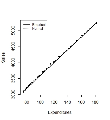
We use a real data set consisting of $CO_{2}$ emission (metric kgs per capita) and energy usage (kg of oil equivalent per capita) of Turkey between the years 1974-2014. The data set can be obtained from “https://data.worldbank. org”. The scatter plot in Figure 2(a) show that a linear relationship between logarithms of $CO_{2}$ emission and energy usage. If the error terms are calculated using the LS estimates (-15.06489, 1.16258), it can be seen that the data has AR(1) structure with $\hat{\phi}=0.65$ autocorrelation coefficient, since the Durbin-Watson test statistic and its p-value are 0.662571 and 1.235e-07,respectively. The ACF (autocorrelation function) and PACF (Partial ACF) plots given in Figure 3 also support the same results. Further, Q-Q plot of residuals in Figure 3 yield that the assumption of normally distributed error terms is achieved.

For this data set,we use the CML and CEL estimates to estimate the parameters of regression model and autocorrelation structure and also error variance. Note that the LS estimates of original data are used as initial values to compute the CML and the CEL estimates given in Table Empirical Likelihood Estimation for Linear Regression Models with AR(p) Error Terms. The fitted regression lines along with the scatter plot of original data are also given in Figure 2(a),and we can see that both methods give similar results.

To evaluate the performance of CEL method when there are outliers in the data or departure from normality, we create an artificial outlier multiplying last observation by five in the data, and use the both estimation methods to estimate the model parameters. The estimates are provided in Table Empirical Likelihood Estimation for Linear Regression Models with AR(p) Error Terms and the fitted lines obtained from both methods can be seen in Figure 2(b). We can easily see from Figure 2(b), the CEL method have better fit than the CML method to the data with outlier. Although real autocorrelation is positive, the CML estimate of autocorrelation is calculated as negative because of the outlier effect. In this case the LS estimates of regression parameters are (-27.4952, 2.0717) and estimated autocorrelation is -0.0107.

4 Conclusion

In literature, the CML or the LS methods are often adapted to estimate the parameters of an autoregressive error terms regression model. The CML method are applied to carry on the estimation under some distributional assumption on the error therm. However, for some data sets it may not be plausible to make some distributional assumption on the error term due to the lack of information about data sets. For those data sets, some alternative distributional assumption free methods should be preferred to continue regression analysis. One of those distributional free estimation methods is the EL method, which can also be used for small sample sizes. In this paper, we have used the EL estimation method to estimate the parameters of an autoregressive error terms regression model. We have defined a CEL function and constructed the necessary constraints using probability weights and the normal equations borrowed from the classical LS estimation method to conduct parameter estimation. To evaluate and compare the performance of the proposed method with the CML method we have provided a simulation study and an example. We have compared the results using the MSE and the bias. We have designed two different simulation scenarios, data with outliers and data without outliers. The results of simulation study, numerical and real data examples have demonstrated that the CEL method can perform better than the CML method when there are outliers in the data set, which symbolizes the deviation from normality assumption. On the other hand, they have similar performance if there are no outliers in the data sets.

References

[1] T. Alpuim and A. El-Shaarawi, On the efficiency of regression analysis with AR(p) errors, Journal of Applied Statistics, 35:7(2008),pp.717–737.
[2] C.F. Ansley, An algorithm for the exact likelihood of a mixed autoregressive-moving average process, Biometrika, 66:1 (1979),pp. 59–65.
[3] C.M. Beach and J.G. McKinnon, A maximum likelihood procedure for regression with autocorrelated errors, Econometrica 46:1(1978),pp.51–58.
[4] H.D. Bondell and L.A. Stefanski, Efficient Robust Regression via Two-Stage Generalized Empirical Likelihood, Journal of the American Statistical Association, 108:502 (2013),pp. 644–655,.
[5] S.X. Chen,On the accuracy of empirical likelihood confidence regions for linear regression model, Ann. Inst. Statist. Math., 45 (1993),pp. 621–637.
[6] S.X. Chen,Empirical likelihood confidence intervals for linear regression coefficients, J. Multiv. Anal., 49 (1994), pp. 24–40.
[7] S.X. Chen, Empirical likelihood confidence intervals for nonparametric density estimation, Biometrika, 83 (1996),pp. 329–341.
[8] S.X. Chen and H. Cui, An extended empirical likelihood for generalized linear models, Statist. Sinica, 13 (2003), pp. 69–81.
[9] S.X. Chen, and I.V. Keilegom, A review on empirical likelihood methods for regression, TEST, 19:3 (2009),pp.415–447.
[10] P. Hall and B. La Scala, Methodology and algorithms of empirical likelihood, Internat. Statist. Review, 58(1990),pp. 109–127.
[11] E. D. Kolaczyk, Empirical likelihood for generalized linear model, Statist. Sinica, 4 (1994),pp. 199–218.
[12] D.C. Montgomery, E.A. Peck and G.G. Vining, Introduction to linear regression analysis (Vol. 821). John Wiley & Sons, 2012.
[13] W. Newey and R.J. Smith, Higher-order properties of GMM and generalized empirical likelihood estimators, Econometrica, 72 (2004),pp. 219–255.
[14] A.B. Owen, Empirical likelihood ratio confidence intervals for a single functional, Biometrika, 75(1988),pp. 237-249.
[15] A.B. Owen, Empirical likelihood confidence regions, Ann. Statist., 18(1990),pp. 90–120.
[16] A.B. Owen, Empirical likelihood for linear models, Ann. Statist., 19(1991),pp. 1725–1747.
[17] A.B. Owen, Empirical Likelihood, Chapman and Hall, New York,2001.
[18] A.B. Owen, Self-concordance for empirical likelihood, Canadian Journal of Statistics, 41:3 (2013),pp. 387-397.
[19] Ş. Özdemir and O. Arslan,An alternative algorithm of the empirical likelihood estimation for the parameter of a linear regression model, Communications in Statistics - Simulation and Computation,48:7 (2019), 1913-1921.
[20] Ş. Özdemir and O. Arslan, Combining empirical likelihood and robust estimation methods for linear regression models, Communications in Statistics - Simulation and Computation,(2019). Available at https://www.tandfonline.com/doi/full/10.1080/03610918.2019.1659968
[21] R Core Team, R: A Language and Environment for Statistical Computing, (2017). Available at https://www.R-project.org/
[22] J. Shi and T.S. Lau, Robust empirical likelihood for linear regression models under median constraints, Communications in Statistics: Theory and Methods,28:10 (1999), pp. 2465–2476.
[23] J. Qin and J. Lawless, Empirical likelihood and general estimating equations, Ann. Statist., 22(1994), pp. 300–325.
[24] M.L. Tiku, W. Wong and G. Bian, Estimating parameters in autoregressive models in nonnormal situations: Symmetric innovations, Communications in Statistics: Theory and Methods, 28:2(1999),pp. 315–341.
[25] Y. Tuaç, Y. Güney, B. Şenoğlu and O. Arslan, Robust parameterestimation of regression model with AR(p) error terms, Communications in Statistics - Simulation and Computation, 47:8(2018), pp. 2343–2359.
[26] Y. Tuaç, Y. Güney and O. Arslan,Parameter estimation of regression model with AR(p) error terms based on skew distributions with EM algorithm, Soft Computing, (2019).Available at https://doi.org/10.1007/s00500-019-04089-x
[27] D. Yang and D.S. Small, An R package and a study of methods for computing empirical likelihood, Journal of Statistical Computation and Simulation, 83:7 (2013),pp. 1363–1372.

\tbl

Estimates, MSE and Bias values of the estimates from $a_{t}\sim N(0,1)$ for different sample sizes without outliers. True values are $(\beta_{1},\beta_{2},\beta_{3})^{\prime}=(1,3,5)^{\prime}$ , $(\phi_{1},\phi_{2})^{\prime}=(0.8,-0.2)$ and $\sigma^{2}=1$ n=25 n=50 n=100 Normal Empirical Normal Empirical Normal Empirical $\hat{\beta}_{1}$ 0.98796 1.00138 0.99845 1.00178 0.99932 1.00068 $\beta_{1}$ MSE 0.03276 0.0058 0.01445 0.00228 0.00584 0.00074 BIAS 0.14255 0.05276 0.09522 0.0319 0.0605 0.01832 $\beta_{2}$ $\hat{\beta}_{2}$ 3.00136 3.00697 2.99808 3.00009 2.9978 2.99753 MSE 0.03247 0.00613 0.01346 0.00225 0.00664 0.00071 BIAS 0.14406 0.05512 0.09181 0.03214 0.06437 0.01797 $\hat{\beta}_{3}$ 5.00803 5.00139 4.99681 4.99966 4.99913 5.00266 $\beta_{3}$ MSE 0.03481 0.00657 0.01421 0.00202 0.00583 0.00069 BIAS 0.14491 0.05574 0.09389 0.03042 0.06045 0.01789 $\phi_{1}$ $\hat{\phi}_{1}$ 0.76906 0.80372 0.77997 0.8013 0.79587 0.80081 MSE 0.0457 0.00028 0.02118 0.0001 0.01042 0.00004 BIAS 0.16869 0.01328 0.11537 0.00784 0.08196 0.00465 $\hat{\phi}_{2}$ -0.2095 -0.19714 -0.20945 -0.199 -0.21079 -0.20002 $\phi_{2}$ MSE 0.04266 0.00029 0.01949 0.0001 0.00951 0.00004 BIAS 0.16559 0.01394 0.11067 0.00824 0.07779 0.00467 $\sigma^{2}$ $\hat{\sigma}^{2}$ 0.88229 1.15221 0.94378 1.1022 0.96983 1.07259 MSE 0.03511 0.03062 0.01351 0.01454 0.00633 0.00784 BIAS 0.15368 0.15458 0.09334 0.1022 0.06461 0.07326

\tbl

Estimates, MSE and Bias values of the estimates for different sample sizes from $a_{t}\sim 0.9N(0,1)+0.1N(30,1)$ . True values are $(\beta_{1},\beta_{2},\beta_{3})^{\prime}=(1,3,5)^{\prime}$ , $(\phi_{1},\phi_{2})^{\prime}=(0.8,-0.2)$ and $\sigma^{2}=1$ n=25 n=50 n=100 Normal Empirical Normal Empirical Normal Empirical $\hat{\beta}_{1}$ 0.99758 1.0001 1.01599 1.0008 0.9947 1.00067 $\beta_{1}$ MSE 0.53329 0.00588 0.11102 0.00189 0.02944 0.00071 BIAS 0.56527 0.05219 0.26139 0.02957 0.13598 0.01776 $\beta_{2}$ $\hat{\beta}_{2}$ 2.97227 3.00938 2.98684 2.9988 2.99961 3.00186 MSE 0.51638 0.00659 0.10983 0.00222 0.02613 0.00068 BIAS 0.5623 0.05636 0.26129 0.03185 0.12822 0.01766 $\hat{\beta}_{3}$ 4.97749 5.00772 5.00388 5.00511 4.99569 5.00152 $\beta_{3}$ MSE 0.50668 0.00559 0.10949 0.00218 0.0282 0.00072 BIAS 0.55812 0.05204 0.2574 0.03174 0.13337 0.01798 $\phi_{1}$ $\hat{\phi}_{1}$ 1.77218 0.80245 1.7009 0.80143 1.63445 0.80104 MSE 0.9494 0.00029 0.81299 0.00009 0.69691 0.00003 BIAS 0.97218 0.0136 0.9009 0.00746 0.83445 0.00446 $\hat{\phi}_{2}$ -0.94992 -0.19518 -0.75483 -0.19879 -0.64632 -0.20002 $\phi_{2}$ MSE 0.58956 0.00033 0.31046 0.00011 0.19993 0.00004 BIAS 0.74992 0.01471 0.55483 0.0083 0.44632 0.00462 $\sigma^{2}$ $\hat{\sigma}^{2}$ 5.95214 1.13923 4.42534 1.10108 3.30909 1.06915 MSE 24.68756 0.02581 11.7763 0.0142 5.34667 0.00688 BIAS 4.95214 0.1419 3.42534 0.10183 2.30909 0.06921

\tbl

Estimates, MSE and Bias values of the estimates for different sample sizes from $a_{t}\sim 0.9N(0,1)+0.1N(0,10)$ . True values are $(\beta_{1},\beta_{2},\beta_{3})^{\prime}=(1,3,5)^{\prime}$ , $(\phi_{1},\phi_{2})^{\prime}=(0.8,-0.2)$ and $\sigma^{2}=1$ n=25 n=50 n=100 Normal Empirical Normal Empirical Normal Empirical $\hat{\beta}_{1}$ 1.00012 1.00766 0.9878 0.99887 0.99299 1.00153 $\beta_{1}$ MSE 0.21859 0.00777 0.11943 0.00276 0.06829 0.00076 BIAS 0.33632 0.05886 0.26183 0.034 0.20502 0.01859 $\beta_{2}$ $\hat{\beta}_{2}$ 2.99806 2.9978 2.98896 3.00449 2.98302 3.00347 MSE 0.23989 0.0086 0.13169 0.00265 0.06363 0.00083 BIAS 0.34908 0.06087 0.2692 0.03391 0.19512 0.01922 $\hat{\beta}_{3}$ 5.01594 5.00257 4.99975 5.00495 4.99407 4.99616 $\beta_{3}$ MSE 0.22748 0.0079 0.12487 0.00273 0.06541 0.00083 BIAS 0.3443 0.05964 0.26638 0.03409 0.19757 0.01894 $\phi_{1}$ $\hat{\phi}_{1}$ 0.79014 0.80161 0.73106 0.80076 0.7298 0.80066 MSE 0.43476 0.00022 0.18784 0.00009 0.08888 0.00004 BIAS 0.51506 0.01213 0.34467 0.00757 0.23919 0.00471 $\hat{\phi}_{2}$ -0.46927 -0.19645 -0.26362 -0.19819 -0.21955 -0.19966 $\phi_{2}$ MSE 0.7917 0.00031 0.23481 0.0001 0.08613 0.00004 BIAS 0.70074 0.01421 0.37436 0.00786 0.23868 0.00473 $\sigma^{2}$ $\hat{\sigma}^{2}$ 2.65719 1.14735 2.70776 1.09725 2.94881 1.06939 MSE 3.79346 0.02846 3.59029 0.01368 4.16932 0.00702 BIAS 1.65951 0.14943 1.70791 0.09889 1.94881 0.0697

\tbl

The parameter estimates for soft drink data without outlier with one outlier Empirical Normal Empirical Normal $\hat{\beta}_{0}$ 1593.95911 1645.37912 1617.57068 560.9601 $\hat{\beta}_{1}$ 20.07335 19.80988 19.93477 30.7569 $\hat{\phi}_{1}$ 0.89579 0.56856 0.89814 -2.5689 $\hat{\sigma}^{2}$ 6.43127 16.96544 2.44785 2025.174

\tbl

The parameter estimates for $CO_{2}$ emission-Energy usage data without outlier with one outlier Empirical Normal Empirical Normal $\hat{\beta}_{0}$ -15.389316 -13.827491 -13.891223 -25.869536 $\hat{\beta}_{1}$ 1.187502 1.074341 1.076084 1.952316 $\hat{\phi}_{1}$ 0.655439 0.861551 0.511249 -0.201119 $\hat{\sigma}^{2}$ 0.824727 0.021447 1.148087 0.900177