Emergent strongly coupled ultraviolet fixed point in four dimensions with 8 Kähler-Dirac fermions
Abstract
The existence of a strongly coupled ultraviolet fixed point in 4-dimensional lattice models as they cross into the conformal window has long been hypothesized. The SU(3) gauge system with 8 fundamental fermions is a good candidate to study this phenomenon as it is expected to be very close to the opening of the conformal window. I study the system using staggered lattice fermions in the chiral limit. My numerical simulations employ improved lattice actions that include heavy Pauli-Villars (PV) type bosons. This modification does not affect the infrared dynamics but greatly reduces the ultraviolet fluctuations, thus allowing the study of stronger renormalized couplings than previously possible. I consider two different PV actions and find that both show an apparent continuous phase transition in the 8-flavor system.
I investigate the critical behavior using finite size scaling of the renormalized gradient flow coupling. The finite size scaling curve-collapse analysis predicts a first order phase transition consistent with discontinuity exponent in the system without PV bosons. The scaling analysis with the PV boson actions is not consistent with a first order phase transition. The numerical data are well described by ”walking scaling” corresponding to a renormalization group function that just touches zero, , though second order scaling cannot be excluded. Walking scaling could imply that the 8-flavor system is the opening of the conformal window, an exciting possibility that could be related to t’Hooft anomaly cancellation of the system.
I Introduction
The existence of a conformal phase in 4-dimensional gauge-fermion systems is well established [1]. The upper limit of the fermion number where the conformal phase becomes infrared free can be predicted perturbatively. However, the lower limit where the QCD-like chirally broken and confining phase turns conformal requires a non-perturbative approach. The conformal phase is characterized by an infrared fixed point (IRFP) where the gauge coupling is irrelevant. In the “walking technicolor” scenario the conformal window opens up when the renormalization group (RG) function vanishes just before chiral symmetry breaking could decouple the fermions [2, 3, 4, 5, 6]. This fixed point turns into an IRFP as the number of fermions is further increased, but at the sill the function has a maximum that just touches zero. Alternatively, the IRFP could appear together with an ultraviolet fixed point (UVFP) as hypothesized by several authors [7, 8, 9, 10]. At the sill of the conformal window the function is similar to that of the walking scenario. The difference becomes evident in the conformal regime where the function exhibits both an IRFP and a UVFP. Conformality is ”lost” as the two fixed points merge and move into the complex plane. This latter scenario is particularly interesting as the emergence of a UVFP implies a second order phase transition with a new relevant operator. The corresponding phase diagram of the conformal regime was sketched in Ref.[11] and reproduced in the left panel of Fig.1. The sketch shows the phase structure and the RG flows in an extended parameter space that includes a new relevant operator denoted by . As the number of flavors increases the IRFP moves to weaker coupling. When the Gaussian FP (GFP) and the IRFP merge, the system becomes infrared free. On the other hand, when the number of flavors decreases, the IRFP approaches the UVFP. The opening of the conformal window is characterized by the merge of the UV and IR fixed points, as is sketched on the right panel of Fig.1.


The conformal IRFP does not separate phases. However, a UVFP would be associated with a continuous phase transition, indicated by the solid black curves in Fig.1. The phase transition might turn to first order before it intercepts the action, if the two lines intercept at all (dashed black curves in Fig.1.). Phase transitions are much easier to identify in numerical simulations than RG fixed points. QCD-like, chirally broken lattice models often do not show any phase transition at zero temperature. When they do (e.g. with Wilson fermions), it is a bulk first order transition that arises from lattice artifacts. Conformal lattice systems, on the other hand, almost always exhibit a phase transition from the conformal phase at weak coupling to a confining one in the strong coupling regime. However, despite extensive numerical studies of systems with various fermion flavors, representations, and gauge colors, no continuous phase transition has been identified in four dimensional gauge-fermion systems at zero temperature. For a recent review see e.g. [12] and references therein.
In this paper, I present numerical results that indicate a continuous phase transition of an SU(3) gauge model with 8 fundamental massless fermions implemented as two sets of staggered lattice fields. This system has been investigated by several collaborations using different versions of staggered fermions [13, 14, 15, 16, 17, 18, 19, 20, 21, 22, 23, 24]. Lattice results indicate that is close to the conformal sill, though there is no solid evidence that would show if it is inside or out of the conformal window. For example, finite temperature simulations at zero fermion mass do not identify a chirally broken phase before the appearance of a first order bulk transition [13, 17, 21]. Spectrum results in the weak coupling regime are consistent with dilaton chiral perturbation theory (dChiPT), which is designed to describe systems very close but below the conformal sill [25, 23, 26, 27, 28]. However, dChiPT fits found that the extrapolation of the lattice data to the chiral limit is very long, and the dynamically-generated IR scale of the massless Nf=8 theory is much smaller than all the scales probed by simulations. It is also feasible that dChiPT describes systems very close but above the conformal sill[29].
Staggered fermions are equivalent to Dirac-Kähler fermions and correspond to four Dirac flavors per staggered species at the vanishing gauge coupling of the Gaussian FP [30, 31, 32]. The renormalized trajectory (RT) that originates from the GFP preserves this property, so staggered fermions describe Dirac flavors around the GFP, and even at the IRFP, if the system is conformal. Beyond the IRFP the equivalence does not have to hold.
Most of the existing studies with 2 staggered fields found a first order bulk transition, and many identified a novel strong coupling phase that exhibits spontaneous breaking of the single-site shift symmetry of staggered fermions (S4 phase) [33]. The S4 phase appears to be chirally symmetric and confining 111 The spectrum in the S4 phase has been studied extensively with flavors (3 staggered fermions) in Ref. [33]. In the case only the existence of the phase as evidenced by the S4 order parameter has been established. Simulations with finite fermion mass in the S4 phase are under way and publication describing the meson spectrum is in preparation., conceivably describing symmetric mass generation (SMG) [34, 35, 36]. Two staggered fermion species in the massless limit are equivalent to four reduced staggered fields that correspond to 16 Weyl spinors. This is exactly the fermion number needed to cancel all t’Hooft anomalies, a necessary condition for the fermions to become massive while remaining chirally symmetric. Thus the model could describe SMG if an appropriate four-fermion interaction is induced [35, 36]. Gauge fields with momentum close to the cutoff might generate such interaction between the fermion doublers. This possibility has not been pursued since a universal continuum limit cannot be defined at first order phase transitions. The existence of a continuous phase transition would change the picture.
The results I present here were obtained using uniquely improved lattice actions that contain heavy Pauli-Villars (PV) type bosonic fields [37], similar to the PV regulators in perturbation theory [38]. The mass of the PV bosons is always kept comparable to the cutoff, thus the PV fields do not influence the IR dynamics. However, they generate a local effective gauge action that shifts the bare gauge coupling towards weaker coupling where the UV fluctuations are suppressed. As the number of PV fields increases, or their mass decreases, the bulk phase transition is also shifted. Both in Ref. [37] and in the present work it is observed that the renormalized gauge coupling increases, while the discontinuity decreases at the phase transition as PV bosons are added. In the system the discontinuity at the phase transition eventually disappears, suggesting a continuous transition. This could imply that the first order transition observed without PV bosons at strong coupling is due to lattice fluctuations and opens the possibility that a non-perturbative, strongly coupled UVFP emerges as the cutoff effects are reduced by improved actions.
I investigate two lattice actions with different PV boson contents, in addition to the one without PV fields. I use finite size scaling to predict the critical coupling and the critical exponent at the phase transition. In the analysis I use the finite volume gradient flow renormalized coupling [39] at various flow times fixed by the lattice size as , where is an arbitrary parameter that I vary between 0.3 and 1.0, though the conclusion is based on the results at [40]. Inspired by the arguments in Refs. [2, 7, 9], I also consider a scaling form corresponding to an RG function that touches the axis at , i.e. . This is reminiscent to the Berezinsky, Kosterlitz, Thouless (BKT) scaling of the 2 dimensional XY model, though with exponent , instead of [41, 42, 43]. The finite size scaling analysis for the action without PV bosons is consistent with a first order transition with critical exponent close to 1/4. The PV improved actions show good curve collapse and consistent exponents for for “walking scaling” and , though second order scaling cannot be fully excluded either. However, numerical results of the PV improved actions are not consistent with a first order transition.
The rest of this paper is organized as follows. Sect. II.1 describes the lattice actions and the effect of the additional PV bosons. In Sect. II.2 I outline finite size scaling with the gradient flow coupling and discuss the relevant scaling forms. Sect. III.1 compares the phase structure of the PV improved actions and the original action without PV fields. Finally, I present the result of the finite size scaling analysis in Sect. III.2. Sect. IV summarizes the results and discusses open questions.
II Lattice definitions
II.1 The PV lattice action
I use a gauge action that includes fundamental and adjoint plaquette terms with couplings and , related by [33]. The gauge links in the staggered fermion operator are nHYP-smeared [44, 45] with smearing parameters . This lattice action has been used in multiple 8-, 4+8, and 12-flavor works [33, 17, 20, 46, 47, 48, 49], including the large-scale spectrum studies of the LSD collaboration [50, 51].
In the simulations I set the fermion mass to and use symmetric volumes with , 10, 12, 16, and 20. The fermion boundary condition is antiperiodic in all four directions to control the fermion zero modes. The gauge fields obey periodic boundary conditions. Simulations with are well behaved in conformal systems or in the small volume deconfined regime of QCD-like systems. The S4 phase is confining but chirally symmetric, and the pions are not particularly light [33]. While numerical simulations are increasingly difficult at strong gauge coupling, the Hybrid Monte Carlo (HMC) updates are well controlled even in the chiral limit of the S4 phase.
For each staggered fermion field, I include PV bosons. The PV bosons have the same action as the fermions but with bosonic statistics [37]. They are degenerate in mass and I choose their lattice mass to be much larger than any IR scale of the system. When integrated out, the PV fields generate an effective gauge action. This is not an ultra-local action, but still local, with localization governed by the mass of the PV “pions”. With heavy PV mass the bound state meson masses are approximately , i.e. the range of the effective gauge action is a few lattice spacings if . The leading term of the induced gauge action is a plaquette built from smeared links with coefficient
| (1) |
where is the number of staggered fermion fields. Since is negative, the bare gauge coupling has to increase to keep the effective gauge coupling and the lattice spacing constant. In general, more PV bosons and/or smaller values generate a larger induced gauge action. The constant physics regime is pushed to weaker bare gauge coupling, which reduces the ultraviolet fluctuations as evidenced by larger plaquette expectation values. The effect of the PV bosons was investigated in detail in Ref. [37] for the 12-flavor SU(3) system. I want to emphasize that the effect of the PV bosons in the simulations is the generation of a local effective gauge action. The corresponding system has the same infrared properties at the Gaussian, as well as other possible fixed points as the original action, as long as and .
II.2 Finite size scaling with gradient flow
The nonperturbative UVFP in the 8-flavor SU(3) gauge system, if it exists, has at least two relevant parameters, the fermion mass and the new operator emerging at the UVFP. The scaling forms I consider below assumes the simplest scenario, i.e. that there are exactly two relevant parameters. If the fermion mass is set to zero, the RG flow is restricted to the critical surface of the massless theory. In that case, the UVFP has only one relevant operator, and finite size scaling methods can be used to study its properties. This is the scenario depicted in the sketches of Fig. 1.
Finite size scaling studies usually consider susceptibilities or bound state masses obtained from 2-point functions. Here I use the gradient flow coupling . The gradient flow (GF) [52, 53]. is a smoothing transformation that has been used extensively in lattice studies GF is not an RG transformation as it lacks the essential coarse-graining step. However, coarse-graining can be implemented at the level of expectation values. If one relates the lattice GF time to the RG scale change as , at large the GF can be interpreted as a well-defined real-space RG transformation [54]. Observables at finite flow time correspond to RG flowed observables at energy scale , and exhibit hyperscaling in the vicinity of an RG fixed point.
The GF coupling was proposed in Ref. [39] for scale setting and in Ref. [40] to calculate the finite volume step scaling function in QCD-like or conformal system. It is defined as
| (2) |
where is the energy density at bare gauge coupling and flow time on lattice volume 222If , where refers to color, matches the coupling at tree level perturbation theory [39]. In the non-perturbative phase this normalization is arbitrary, but I keep it for consistency.. In lattice calculations various local operators like the plaquette or the clover operator can be used to approximate . A frequent choice to estimate is
| (3) | |||
| (4) |
where and denote the expectation value of the plaquette before GF flow and at flow time . The GF defines a non-linear RG transformation, therefore does not have an anomalous dimension, i.e. the exponent of the RG does not enter. Thus, the scaling dimension of the gradient flow coupling vanishes, its RG evolution depends only on the RG flow in the action parameter space.333The use of to approximate is reminiscent of the operators used in Monte Carlo Renormalization Group (MCRG) studies [55, 56, 57, 58]. The main difference is that GF is continuous, so one is not restricted to scale change of 2. Also, the lattice volume does not decrease during GF, so larger flow time/ RG scale change is possible. . This property greatly simplifies the RG scaling relations, as only the scaling exponent related to the correlation length enters.
One can think of as a scalar quantity that tracks the renormalized trajectory [59, 11]. It has several advantages, most important is that it is a simple expectation value that is easy to measure with high precision. Finite size scaling relations for are derived in the usual way. At a second order phase transition one expects the correlation length to scale as
| (5) |
where denotes the critical coupling. The combination
| (6) |
is a dimensionless scaling variable. Renormalization group scaling in finite volume therefore implies that , , depends on , i.e. follows a unique but a priori unknown scaling function
| (7) |
First order phase transitions are expected to show similar scaling behavior but with discontinuity exponent in 4 dimensions.
If the RG -function behaves as
| (8) |
in the vicinity of the critical point, the phase transition is continuous but “walking” or BKT-type. The correlation length scales as
| (9) |
and the corresponding scaling function depends on ,
| (10) |
The 2-dimensional XY model has , while the quadratic “walking” function in Eq. 8 corresponds to . Both Eqs. 7 and 10 are leading order relations valid only in the vicinity of the critical point, . One also has to assure that the flow does not drive the RG blocked correlation length below the lattice spacing, . At the same time has to be large enough for the RG flow to reach the renormalized trajectory. This latter condition could limit the use of the smallest volumes, since and is commonly preferred444At larger values the GF “wraps around” the finite volume. That does not invalidate the use of , though the statistical errors increase with increasing . A full investigation on the dependence on , similar to Ref.[60], is a worthwhile project for the future. . The RT is approached according to the largest non-leading exponent, but corrections to scaling could be important. This, however, is beyond what my present data set can describe.
The scaling functions and depend on the parameter , but should not depend on , , and . In addition, different lattice actions should show scaling with the same exponent, though and are dependent on the action. Thus testing different values and different actions provides a consistency check and verifies the scaling form.
III Numerical results
III.1 The phase structure


I investigated several different PV boson actions, two of them in detail. The first one contains 8 PV fields for each staggered flavor with mass (8PV-m0.75 action), and the second one contains 4 PV fields per staggered flavor with mass (4PV-m0.5 action). I have also looked at the action without PV bosons (0PV action). The 0PV action was studied previously in Ref. [17] at small but finite mass, and in the chiral limit but at weaker couplings in Ref. [20]. No previous work considered the 8-flavor systems at the phase transition directly in the chiral limit. In contrast, all simulations I present here are performed with .
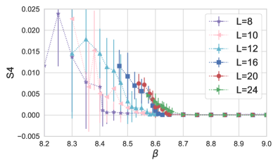
I start by comparing the plaquette expectation value, the finite volume GF coupling, the S4 order parameter for the plaquette, and the topological susceptibility of the three actions. The top panel of Fig. 2 shows the plaquette as the function of the bare gauge coupling on volumes , 10, 12, 16, and 20 for the 0PV action. The discontinuity at the phase transition is too small to be resolved on the plot. Nevertheless, I have observed tunneling and 2-state signals in several ensembles, consistent with a first order phase transition. The GF coupling at is shown on the second panel. It exhibits a rapid change around on these volumes, consistent with a phase transition around , the value predicted with small but finite fermion masses in Ref.[17]. The strong coupling phase exhibits spontaneous breaking of the staggered single-site shift symmetry (S4 phase). The S4 order parameter that measures the staggered nature of the plaquette (Eq. 3. in Ref. [33]) is shown on the third panel. It is fairly noisy but useful to verify that the new phase shows the S4 symmetry breaking pattern. The S4 phase is confining but chirally symmetric, and the existence of a local order parameter ensures that it is separated from both the conformal and the chirally broken, confining phases by a phase transition [33] The bottom panel of Fig. 2 shows the topological susceptibility . In the chiral limit of conformal and QCD-like systems one expects , because the fermion determinant has a zero mode on isolated instantons. Staggered fermion lattice artifacts lift slightly at finite lattice spacing [61]. However, in the S4 phase, the topological charge is large and no longer suppressed. This is further evidence of the very different nature of this new phase.
The largest GF coupling in the weak coupling phase of the 0PV model is with and . The plaquette is fairly small at the phase transition, (normalized to 3.0), suggesting large UV fluctuations. This system has another first order phase transition at an even stronger coupling that separates the S4 phase from a QCD-like chirally broken, confining regime [17]. I am not concerned with that transition in this work.
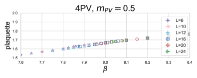
The panels of Figs. 3 and 4 show the same quantities as Fig. 2 but for the 8PV-m0.75 and 4PV-m0.5 actions and volumes 555Simulations with the PV actions are computationally faster, similar to the observation presented in Table I of Ref. [37] for , thus larger volumes are feasible.. The GF coupling now appears continuous. None of my numerical simulations showed 2-state signals or phase tunneling either. The S4 order parameter becomes non-zero at the same place where shows a qualitative change of dependence, around , . This is also where the S4 order parameter and topological susceptibility show a sudden increase. The plaquette is significantly larger at the phase transition, and , respectively. The bare gauge coupling of the phase transition has also shifted to larger bare coupling, from of the 0PV action to and . This is the consequence of the induced effective action.
The strongest GF coupling with the 0PV action is on the volumes considered, compared to with both PV actions. The 0PV action has large vacuum fluctuations. It appears that those trigger a first order phase transition before the GF coupling is strong enough to undergo the continuous transition seen with the 4PV-m0.5 and 8PV-m0.75 actions. This suggests that the first order phase transition could be only a lattice artifact. The picture is similar to the frequently observed first order bulk transition with Wilson fermions that are not considered physical.


If the phase transition is continuous, it should follow a scaling form like Eq. 7 or Eq. 10. A first order phase transition should follow the scaling of Eq. 7 with exponent . The critical coupling , exponent and parameter can be determined based on a curve collapse analysis of vs. or , respectively. I perform this analysis similar the Nelder-Mead method as described in [62].
Specifically, I chose a reference volume and interpolate versus with a (smoothed) cubic spline. In the analysis below I use . I fit the parameters , (and ) by minimizing the deviation of from this interpolating curve at , where is the solution of the equation
| (11) |
if fitting Eq. 7 or
| (12) |
if fitting Eq. 10 The procedure can be iterated by refining the “ideal” interpolating curve using more volumes, once the fit parameters are known approximately.
III.1.1 Second order scaling test
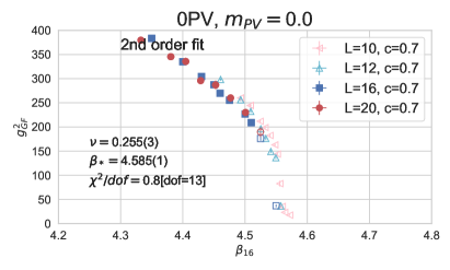
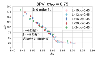
Fig. 5 shows the curve collapse analysis for the three actions based on the second order scaling form of Eq. 7 at and . I included only in the fit. In addition, I excluded those data points that are not clearly in the S4 phase666 At a first order phase transition the critical coupling of an MCRG approach can overshoot the discontinuity, especially if the transition is strongly first order [63, 64]. In order to avoid data that are in the weak coupling phase I employ a conservative cut based on the S4 order parameter.. However, for completeness, I show the smaller volumes and excluded data points in Fig. 5 using open symbols. The top left panel shows the curve collapse for the 0PV action. The fit with predicts , close to the expected first order value with . The fit with predicts , even closer to the expected discontinuity exponent, with similarly small . The predicted critical couplings are consistent, and 4.585(1), and compatible with the data in Fig. 2 and the observed phase transition in Ref.[21]. The bottom two panels show the curve collapse for the two PV improved actions. Again, only are included in the fit. In all cases is , but the predicted exponent varies between 0.53 and 0.63, very different from the discontinuity exponent of a first order phase transition.
To test the consistency of the curve collapse, I repeat the analysis varying the parameter between 0.3 and 1.0. I also compare fits using volumes or for the PV actions. Fig. 6 summarizes the predicted and corresponding values for the three actions. The observable drift at smaller indicates that the RG flow has not yet reached the vicinity of the renormalized trajectory. The 0PV action stabilizes at and predicts , the expected scaling exponent at a first order transition. The exponent for the PV improved actions drift and show significant variation depending on the action even at . I do not find a consistent scaling fit with volumes , though it is possible that on larger volumes the curve collapse analysis would predict a consistent exponent, possibly around . For both PV improved actions, a first order transition is not consistent with the numerical data.


III.2 Finite size scaling analysis
III.2.1 “Walking” scaling test
The “walking” or BKT-like scaling form given in Eq. 10 assumes that the RG function just touches zero. This fit form has three free parameters, though is the theoretically motivated value [7]. Using volumes I am able to fit all three parameters. Fig. 7 shows the result of the curve collapse fits for both PV actions at and 0.70. As before, the open symbol data points are not included in the fit. All fits predict consistent with the expected 1.0 value with small and consistent and values.
The predicted fit parameter values are shown in Fig. 8 for different values in the range and volumes and . They all show consistent results.
Fits with BKT-like scaling have smaller than the second-order scaling. The predicted exponent and no significant dependence on also favors the “walking” scaling scenario. However the second order scaling form discussed in Sect. III.1.1 is not excluded. It is well known that corrections to BKT scaling in the 2-dimensional XY model are very large [65]. In the 8-flavor system I have concentrated on fitting the leading terms only. More sophisticated curve collapse fitting, better statistics, and especially larger volumes might allow distinguishing the two cases in the future [66].
IV Summary
I have investigated the SU(3) gauge model with two sets of staggered fermions in the chiral limit. Staggered lattice fermions are equivalent to Dirac-Kähler fermions, and in the chiral limit two staggered fields correspond to 16 Weyl spinors. This system could lead to symmetric mass generation if appropriate terms are induced by the strong interaction.
I study two improved lattice actions that contain heavy Pauli-Villars type bosonic fields. Both improved actions shift the first order phase transition of the original system to weaker bare couplings and smooth out the transition. Using finite size scaling methods I showed that the phase transition with both PV improved actions appears continuous. I investigated scaling according to standard second order phase transition, and also “walking” or BKT-like scaling. First order phase transition with is not consistent with the numerical data. While I cannot exclude second order scaling, the curve collapse fit favors “walking” scaling with . A “walking” scaling phase transition could imply that the system is at the sill of the conformal window as sketched on the right panel of Fig. 1. If that is indeed the case, it is likely that the complete t’Hooft anomaly cancellation of the lattice formulation plays an essential role.
The weak coupling phase with all three actions appears chirally symmetric in the volumes considered, i.e. the simulations are well controlled even in the limit with meson spectrum showing chiral symmetry. Simulations at finite fermion mass that contrast the -regime rotator spectrum with the mass-deformed hyperscaling prediction might be required to establish the infrared properties of the weak coupling phase [67, 16]. In this work I concentrate on the order of the phase transition from the strong coupling side and do not directly investigate the infrared properties of the weak coupling phase. The strong coupling regime breaks the single site shift symmetry of the staggered action. The S4 phase could describe symmetric mass generation, where confinement leads to mass generation without breaking chiral symmetry. The existence of a continuous phase transition would allow taking an infinite cutoff continuum limit. This very exciting possibility requires further analytical and numerical studies.
Lattice studies with fundamental flavors also show an S4 phase in the strong coupling. However, my preliminary numerical studies with various PV actions did not show continuous phase transition in that system. t’Hooft anomalies do not cancel with 12 flavors (i.e. three staggered fermions), possibly explaining the difference between 12 and 8 flavors. However, further studies are needed.
If the model with 2 staggered fermions is conformal in the weak coupling regime, 8 fundamental Dirac fermions should also be conformal. The critical properties at the continuous phase transition, however, are not necessarily universal. It would be very interesting to investigate 8 fundamental flavors with improved domain wall fermions that allow the study of the strong gauge couplings where the continuous phase transition with staggered fermions occur.
Acknowledgments
The phase diagram depicted in Fig. 1 came from a discussion with S. Rychkov. I am indebted for his insight that lead to the present investigation. I am grateful to Yigal Shamir for his constructive criticism and suggestions, and to Simon Catterall for discussions about t’Hooft anomaly cancellation and SMG. I have presented preliminary results to the LSD collaboration and benefited from their probing questions when finalizing the manuscript. I thank Oliver Witzel who carefully read an earlier version of this manuscript for his many comments and suggestions.
Computations for this work were carried out in part on facilities of the USQCD Collaboration, which are funded by the Office of Science of the U.S. Department of Energy, the RMACC Summit supercomputer [68], which is supported by the National Science Foundation (awards No. ACI-1532235 and No. ACI-1532236), the University of Colorado Boulder, and Colorado State University, and on the University of Colorado Boulder HEP Beowulf cluster. I thank the University of Colorado for providing the facilities essential for the completion of this work. My reseach is supported by DOE grant DE-SC0010005.
References
- Banks and Zaks [1982] T. Banks and A. Zaks, On the Phase Structure of Vector-Like Gauge Theories with Massless Fermions, Nucl. Phys. B196, 189 (1982).
- Miransky [1999] V. A. Miransky, Dynamics in the conformal window in QCD like theories, Phys. Rev. D 59, 105003 (1999), arXiv:hep-ph/9812350 .
- Appelquist et al. [1997] T. Appelquist, J. Terning, and L. C. R. Wijewardhana, Postmodern technicolor, Phys. Rev. Lett. 79, 2767 (1997), arXiv:hep-ph/9706238 .
- Appelquist and Bai [2010] T. Appelquist and Y. Bai, A Light Dilaton in Walking Gauge Theories, Phys. Rev. D 82, 071701 (2010), arXiv:1006.4375 [hep-ph] .
- Golterman and Shamir [2016] M. Golterman and Y. Shamir, Low-energy effective action for pions and a dilatonic meson, Phys. Rev. D 94, 054502 (2016), arXiv:1603.04575 [hep-ph] .
- Golterman and Shamir [2018] M. Golterman and Y. Shamir, Large-mass regime of the dilaton-pion low-energy effective theory, Phys. Rev. D 98, 056025 (2018), arXiv:1805.00198 [hep-ph] .
- Kaplan et al. [2009] D. B. Kaplan, J.-W. Lee, D. T. Son, and M. A. Stephanov, Conformality Lost, Phys. Rev. D80, 125005 (2009), arXiv:0905.4752 [hep-th] .
- Vecchi [2010] L. Vecchi, The Conformal Window of deformed CFT’s in the planar limit, Phys. Rev. D 82, 045013 (2010), arXiv:1004.2063 [hep-th] .
- Gorbenko et al. [2018] V. Gorbenko, S. Rychkov, and B. Zan, Walking, Weak first-order transitions, and Complex CFTs, JHEP 10, 108, arXiv:1807.11512 [hep-th] .
- Pomarol et al. [2019] A. Pomarol, O. Pujolas, and L. Salas, Holographic conformal transition and light scalars, JHEP 10, 202, arXiv:1905.02653 [hep-th] .
- Hasenfratz and Witzel [2019] A. Hasenfratz and O. Witzel, Continuous function for the SU(3) gauge systems with two and twelve fundamental flavors, PoS LATTICE2019, 094 (2019), arXiv:1911.11531 [hep-lat] .
- Nogradi and Patella [2016] D. Nogradi and A. Patella, Strong dynamics, composite Higgs and the conformal window, Int. J. Mod. Phys. A31, 1643003 (2016), arXiv:1607.07638 [hep-lat] .
- Deuzeman et al. [2008] A. Deuzeman, M. P. Lombardo, and E. Pallante, The Physics of eight flavours, Phys. Lett. B 670, 41 (2008), arXiv:0804.2905 [hep-lat] .
- Deuzeman et al. [2010] A. Deuzeman, M. P. Lombardo, and E. Pallante, Evidence for a conformal phase in SU(N) gauge theories, Phys. Rev. D 82, 074503 (2010), arXiv:0904.4662 [hep-ph] .
- Jin and Mawhinney [2009] X.-Y. Jin and R. D. Mawhinney, Lattice QCD with 8 and 12 degenerate quark flavors, PoS LAT2009, 049 (2009), arXiv:0910.3216 [hep-lat] .
- Fodor et al. [2009] Z. Fodor, K. Holland, J. Kuti, D. Nogradi, and C. Schroeder, Nearly conformal gauge theories in finite volume, Phys. Lett. B 681, 353 (2009), arXiv:0907.4562 [hep-lat] .
- Hasenfratz et al. [2014] A. Hasenfratz, A. Cheng, G. Petropoulos, and D. Schaich, Reaching the chiral limit in many flavor systems, in KMI-GCOE Workshop on Strong Coupling Gauge Theories in the LHC Perspective (2014) pp. 44–50, arXiv:1303.7129 [hep-lat] .
- Aoki et al. [2013a] Y. Aoki, T. Aoyama, M. Kurachi, T. Maskawa, K.-i. Nagai, H. Ohki, A. Shibata, K. Yamawaki, and T. Yamazaki (LatKMI), Walking signals in QCD on the lattice, Phys. Rev. D87, 094511 (2013a), arXiv:1302.6859 [hep-lat] .
- Aoki et al. [2013b] Y. Aoki, T. Aoyama, M. Kurachi, T. Maskawa, K. Miura, et al., A light composite scalar in eight-flavor QCD on the lattice, PoS LATTICE2013, 070 (2013b), arXiv:1309.0711 [hep-lat] .
- Hasenfratz et al. [2015] A. Hasenfratz, D. Schaich, and A. Veernala, Nonperturbative function of eight-flavor SU(3) gauge theory, JHEP 2015, 143, arXiv:1410.5886 [hep-lat] .
- Schaich et al. [2018] D. Schaich, A. Hasenfratz, and E. Rinaldi (Lattice Strong Dynamics), Finite-temperature study of eight-flavor SU(3) gauge theory, , 351 (2018), arXiv:1506.08791 [hep-lat] .
- Fodor et al. [2015] Z. Fodor, K. Holland, J. Kuti, S. Mondal, D. Nogradi, and C. H. Wong, The running coupling of 8 flavors and 3 colors, JHEP 06, 019, arXiv:1503.01132 [hep-lat] .
- Appelquist et al. [2019a] T. Appelquist et al. (Lattice Strong Dynamics), Nonperturbative investigations of SU(3) gauge theory with eight dynamical flavors, Phys. Rev. D 99, 014509 (2019a), arXiv:1807.08411 [hep-lat] .
- Hasenfratz et al. [2022] A. Hasenfratz, C. Rebbi, and O. Witzel, Gradient flow step-scaling function for SU(3) with eight flavors (2022), in preparation.
- Appelquist et al. [2017] T. Appelquist, J. Ingoldby, and M. Piai, Dilaton EFT Framework For Lattice Data, JHEP 07, 035, arXiv:1702.04410 [hep-ph] .
- Appelquist et al. [2020] T. Appelquist, J. Ingoldby, and M. Piai, Dilaton potential and lattice data, Phys. Rev. D 101, 075025 (2020), arXiv:1908.00895 [hep-ph] .
- Golterman et al. [2020] M. Golterman, E. T. Neil, and Y. Shamir, Application of dilaton chiral perturbation theory to , spectral data, Phys. Rev. D 102, 034515 (2020), arXiv:2003.00114 [hep-ph] .
- Appelquist et al. [2021a] T. Appelquist, J. Ingoldby, and M. Piai, Nearly Conformal Composite Higgs Model, Phys. Rev. Lett. 126, 191804 (2021a), arXiv:2012.09698 [hep-ph] .
- Appelquist et al. [2021b] T. Appelquist, R. C. Brower, K. K. Cushman, G. T. Fleming, A. D. Gasbarro, A. Hasenfratz, X.-Y. Jin, E. T. Neil, J. C. Osborn, C. Rebbi, E. Rinaldi, D. Schaich, P. Vranas, and O. Witzel (Lattice Strong Dynamics), Near-conformal dynamics in a chirally broken system, Phys. Rev. D 103, 014504 (2021b), arXiv:2007.01810 [hep-ph] .
- Banks et al. [1982] T. Banks, Y. Dothan, and D. Horn, Geometric fermions, Phys. Lett. B 117, 413 (1982).
- Becher and Joos [1982] P. Becher and H. Joos, The Dirac-Kahler Equation and Fermions on the Lattice, Z. Phys. C 15, 343 (1982).
- Joos [1986] H. Joos, On geometry and physics of staggered lattice fermions, in NATO Advanced Research Workshop on Clifford Algebras and their Applications to Mathematical Physics (1986).
- Cheng et al. [2012] A. Cheng, A. Hasenfratz, and D. Schaich, Novel phase in SU(3) lattice gauge theory with 12 light fermions, Phys.Rev. D85, 094509 (2012), arXiv:1111.2317 [hep-lat] .
- Tong [2021] D. Tong, Comments on Symmetric Mass Generation in 2d and 4d, (2021), arXiv:2104.03997 [hep-th] .
- Butt et al. [2021a] N. Butt, S. Catterall, A. Pradhan, and G. C. Toga, Anomalies and symmetric mass generation for Kähler-Dirac fermions, Phys. Rev. D 104, 094504 (2021a), arXiv:2101.01026 [hep-th] .
- Butt et al. [2021b] N. Butt, S. Catterall, and G. C. Toga, Symmetric Mass Generation in Lattice Gauge Theory, Symmetry 13, 2276 (2021b), arXiv:2111.01001 [hep-lat] .
- Hasenfratz et al. [2021] A. Hasenfratz, Y. Shamir, and B. Svetitsky, Taming lattice artifacts with Pauli-Villars fields, Phys. Rev. D 104, 074509 (2021), arXiv:2109.02790 [hep-lat] .
- Pauli and Villars [1949] W. Pauli and F. Villars, On the invariant regularization in relativistic quantum theory, Rev. Mod. Phys. 21, 434 (1949).
- Lüscher [2010] M. Lüscher, Properties and uses of the Wilson flow in lattice QCD, JHEP 2010, 071, [Erratum: JHEP 2014, 092], arXiv:1006.4518 [hep-lat] .
- Fodor et al. [2012] Z. Fodor, K. Holland, J. Kuti, D. Nogradi, and C. H. Wong, The Yang-Mills gradient flow in finite volume, JHEP 2012, 007, arXiv:1208.1051 [hep-lat] .
- Berezinsky [1971] V. L. Berezinsky, Destruction of long range order in one-dimensional and two-dimensional systems having a continuous symmetry group. I. Classical systems, Sov. Phys. JETP 32, 493 (1971).
- Kosterlitz and Thouless [1973] J. M. Kosterlitz and D. J. Thouless, Ordering, metastability and phase transitions in two-dimensional systems, J. Phys. C 6, 1181 (1973).
- Kosterlitz [1974] J. M. Kosterlitz, The Critical properties of the two-dimensional x y model, J. Phys. C 7, 1046 (1974).
- Hasenfratz and Knechtli [2001] A. Hasenfratz and F. Knechtli, Flavor symmetry and the static potential with hypercubic blocking, Phys. Rev. D64, 034504 (2001), arXiv:hep-lat/0103029 .
- Hasenfratz et al. [2007] A. Hasenfratz, R. Hoffmann, and S. Schaefer, Hypercubic smeared links for dynamical fermions, JHEP 2007, 029, arXiv:hep-lat/0702028 [hep-lat] .
- Hasenfratz and Schaich [2018] A. Hasenfratz and D. Schaich, Nonperturbative function of twelve-flavor SU(3) gauge theory, JHEP 2018, 132, arXiv:1610.10004 [hep-lat] .
- Cheng et al. [2013] A. Cheng, A. Hasenfratz, G. Petropoulos, and D. Schaich, Scale-dependent mass anomalous dimension from Dirac eigenmodes, JHEP 2013, 061, arXiv:1301.1355 [hep-lat] .
- Brower et al. [2016] R. C. Brower, A. Hasenfratz, C. Rebbi, E. Weinberg, and O. Witzel, Composite Higgs model at a conformal fixed point, Phys. Rev. D93, 075028 (2016), arXiv:1512.02576 [hep-ph] .
- Hasenfratz et al. [2017] A. Hasenfratz, C. Rebbi, and O. Witzel, Large scale separation and hadronic resonances from a new strongly interacting sector, Phys. Lett. B773, 86 (2017), arXiv:1609.01401 [hep-ph] .
- Appelquist et al. [2016] T. Appelquist et al. (Lattice Strong Dynamics), Strongly interacting dynamics and the search for new physics at the LHC, Phys. Rev. D 93, 114514 (2016), arXiv:1601.04027 [hep-lat] .
- Appelquist et al. [2019b] T. Appelquist et al. (Lattice Strong Dynamics), Nonperturbative investigations of SU(3) gauge theory with eight dynamical flavors, Phys. Rev. D99, 014509 (2019b), arXiv:1807.08411 [hep-lat] .
- Narayanan and Neuberger [2006] R. Narayanan and H. Neuberger, Infinite phase transitions in continuum Wilson loop operators, JHEP 2006, 064, arXiv:hep-th/0601210 [hep-th] .
- Lüscher [2010] M. Lüscher, Trivializing maps, the Wilson flow and the HMC algorithm, Commun.Math.Phys. 293, 899 (2010), arXiv:0907.5491 [hep-lat] .
- Carosso et al. [2018] A. Carosso, A. Hasenfratz, and E. T. Neil, Nonperturbative Renormalization of Operators in Near-Conformal Systems Using Gradient Flows, Phys. Rev. Lett. 121, 201601 (2018), arXiv:1806.01385 [hep-lat] .
- Swendsen [1979] R. H. Swendsen, Monte Carlo Renormalization Group, Phys. Rev. Lett. 42, 859 (1979).
- Pawley et al. [1984] G. Pawley, R. Swendsen, D. Wallace, and K. Wilson, Monte Carlo Renormalization Group Calculations of Critical Behavior in the Simple Cubic Ising Model, Phys. Rev. B 29, 4030 (1984).
- Bowler et al. [1985] K. C. Bowler, R. D. Kenway, G. S. Pawley, D. J. Wallace, A. Hasenfratz, P. Hasenfratz, U. M. Heller, F. Karsch, and I. Montvay, Monte Carlo Renormalization Group Studies of SU(3) Lattice Gauge Theory, Nucl. Phys. B257, 155 (1985).
- Hasenfratz [2012] A. Hasenfratz, Infrared fixed point of the 12-fermion SU(3) gauge model based on 2-lattice MCRG matching, Phys. Rev. Lett. 108, 061601 (2012), arXiv:1106.5293 [hep-lat] .
- Hasenfratz and Witzel [2020] A. Hasenfratz and O. Witzel, Continuous renormalization group function from lattice simulations, Phys. Rev. D 101, 034514 (2020), arXiv:1910.06408 [hep-lat] .
- Fritzsch and Ramos [2013] P. Fritzsch and A. Ramos, The gradient flow coupling in the Schrödinger Functional, JHEP 10, 008, arXiv:1301.4388 [hep-lat] .
- Follana et al. [2004] E. Follana, A. Hart, and C. T. H. Davies (HPQCD, UKQCD), The Index theorem and universality properties of the low-lying eigenvalues of improved staggered quarks, Phys. Rev. Lett. 93, 241601 (2004), arXiv:hep-lat/0406010 .
- Bhattacharjee and Seno [2001] S. M. Bhattacharjee and F. Seno, A measure of data collapse for scaling, Journal of Physics A: Mathematical and General 34, 6375–6380 (2001).
- Decker et al. [1988] K. Decker, A. Hasenfratz, and P. Hasenfratz, Singular Renormalization Group Transformations and First Order Phase Transitions: Monte Carlo Renormalization Group Results, Nucl. Phys. B 295, 21 (1988).
- Hasenfratz and Hasenfratz [1988] A. Hasenfratz and P. Hasenfratz, Singular Renormalization Group Transformations and First Order Phase Transitions, Nucl. Phys. B 295, 1 (1988).
- Hasenbusch [2005] M. Hasenbusch, The Two dimensional XY model at the transition temperature: A High precision Monte Carlo study, J. Phys. A 38, 5869 (2005), arXiv:cond-mat/0502556 .
- Sale et al. [2022] N. Sale, J. Giansiracusa, and B. Lucini, Quantitative analysis of phase transitions in two-dimensional XY models using persistent homology, Phys. Rev. E 105, 024121 (2022), arXiv:2109.10960 [cond-mat.stat-mech] .
- Hasenfratz [2010] P. Hasenfratz, The QCD rotator in the chiral limit, Nucl. Phys. B 828, 201 (2010), arXiv:0909.3419 [hep-th] .
- Anderson et al. [2017] J. Anderson, P. J. Burns, D. Milroy, P. Ruprecht, T. Hauser, and H. J. Siegel, Deploying rmacc summit: An hpc resource for the rocky mountain region, Proceedings of PEARC17 8, 1 (2017).