Emergent order in a continuous state adaptive network model of living systems
Abstract
Order can spontaneously emerge from seemingly noisy interactions between biological agents, like a flock of birds changing their direction of flight in unison, without a leader or an external cue. We are interested in the generic conditions that lead to such emergent phenomena. To find these conditions, we use the framework of complex networks to characterize the state of agents and their mutual influence. We formulate a continuous state adaptive network model, from which we obtain the phase boundaries between swarming and disordered phases and characterize the order of the phase transition.
Swarming is a collective phenomenon which is encountered in many biological systems, such as schools of fish, swarms of locusts and flocks of birds. Some swarming phenomena in biological systems can be guided by external cues, or a leading individual, but a large variety of biological systems display spontaneously emerging, self-organized group behavior [1]. Even unicellular organisms, such as the bacterium E. coli and the amoeba D. discoideum, have been observed to display such collective behavior [2].
Models of swarm formation can be broadly put into two categories. The first group we call mechanistic models. Their microscopic interactions are solely based on first principles, and they do not encode the tendency to order explicitly. This works well if all microscopic forces that determine the dynamics are known. Such models have been successfully used to describe the dynamics of self propelled particles of different shapes that exhibit exclusion interactions [3, 4, 5]. The second group, that we call heuristic models, are well exemplified by opinion formation in social groups. We know that people can convince others to join their cause. However, we do not yet understand the details of how one individual can cause another to form an opinion, thus we have a need for a heuristic rule that postulates how two individuals can form a consensus. Such heuristic treatment is in general needed when it is clear that there is a microscopic tendency to align, but we do not know the details of interactions; in context of opinion dynamics, such a model was first put forward by Vicsek et al. [6].
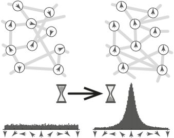
Giving up the connection to the mechanistic first principles opens a door to an interesting opportunity. One can recognize that the heuristic of be more like your neighbor is now the central aspect of the evolution of the system, instead of spatial dynamics of the particles. Thus we are shifting our attention from spatial dynamics to the topology of interactions, a problem for which the language of complex networks is uniquely well suited. In this framework the system is represented by a dynamic network. The agents, corresponding to the nodes of the network, can occupy different states, representing the direction of movement, and the changing topology of the network encodes the temporal dynamics of the interactions. An example of such a system can be seen in fig. 1. One such dynamic network model, for a system with a discrete state space, has been proposed by Chen, Huepe and Gross [7]. This model predicts a first or second order phase transition from a disordered to an ordered state, depending on the number of possible internal states. The first order phase transition has previously been observed in agent based models that follow the spatial dynamics of individuals, and has been confirmed both in experiments with active matter and observations of living systems [8, 9, 10]. The character of the transition can also depend on finite system size effects [11, 12] and on subtle changes in the way the noise is incorporated [13].
Earlier network models [14, 15, 7] have focused on a discrete state space. All the aforementioned biological systems, however, have a continuous state space. Our intuition from equilibrium statistical mechanics tells us that the nature of the state space can matter a lot [16, 17, 18]. It has been demonstrated that in nonequilibrium systems, details affect the type of phase transition. Therefore, in this paper we investigate the swarming transition in a continuous state space.
In this letter we present the numerical solutions of our model accompanied with analytic expressions for the phase space boundary, that we found through stability analysis of the disordered phase. Our results clearly show that continuous state adaptive network models are able to describe spontaneous emergence of order in active systems. We find that the balance of time scales in the model determines the type of phase transition. Our model has two main time scales, the time scale of information propagation through the network, and the time scale of network reshaping. When the latter is significantly faster than the former, we get a mean field like situation, where the network is updated so fast that every node has contact with a random selection of nodes, replacing the link structure by an average connectivity number. The phase transition in this case becomes second order, while in the case that the time scales are of comparable magnitude, we find a first order transition. A meta phase transition between the first and second order regimes, similar to this one has been reported before in the context of active adaptive systems [12].
Model – We model a system of self-propelled particles with a constant speed and changing direction in two dimensions. Each particle corresponds to a node in a network, with an internal state that represents the direction of movement. We represent this internal state by an angle . Nodes may be connected by links, indicating mutual awareness. We will refer to individuals connected by a link as neighbors.
In our system not only the states of individual agents can evolve dynamically, but also the relationship of the agents with their surroundings. Analogously to [7], we distinguish four types of dynamics, given by four rules:
Rule 1 Individuals spontaneously change their heading direction to another uniformly chosen direction with rate .
Rule 2 Individuals adopt to the average direction of two neighbors with rate .
Rule 3 Arbitrarily chosen not-neighboring individuals become neighbors with a coupling rate .
Rule 4 Arbitrarily chosen neighbors loose mutual awareness with a decoupling rate .
An illustration of the model is given in fig. 2. The first two rules are comparable to the rules in the Vicsek model [6]; rule 1 is similar to the noise that is added to each particle’s updated heading direction, whereas rule 2 corresponds to the tendency of individuals to align with their neighbors within a certain radius. The radius is modeled in the network with the links, since we do not keep track of the physical position of individuals in space. The interactions described by rule 3 and rule 4 are needed since non-neighboring individuals, moving in different directions, might become aware of each other and conversely individuals which are neighboring, but head in different directions, may loose mutual awareness; therefore, their link must be created or removed respectively. Since we want to look at the behavior of groups comprised of agents of the same species, we assume that the rates are global.
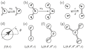
We define the state distribution function which represents the fraction of the agents in the state at time . Thus the integral of over the whole domain is normalized at any time. The cartoon in fig. 1 is an illustration of such a state density that starts out as a random, noisy distribution over the states and evolves into a state corresponding to a collective motion in one predominant direction. Moreover, we define the link distribution function as the density of neighboring individuals, one of which is heading in direction while the other one has direction , at time . Note that in contrast to , the link density is not normalized since the overall number of links can grow or shrink, making the normalization of time dependent. We also define higher order interaction terms like the path-like three node and star-like four node subgraph densities and analogously. A visual representation of these subgraphs can be seen in fig. 2. We note that the link density functions obey certain symmetries. In particular, we have and for higher order terms all non central nodes can be exchanged in any order.
One can derive the master equations for the continuous state model using the four rules, which govern the dynamics of the state and link density distributions. These equations can be interpreted as the extension of the master equations in [7], into the continuous state set.
| (1a) | ||||
| (1b) | ||||
The first term of eq. 1a scales with and models the spontaneous direction changes of nodes. in the second term is a functional that describes three-body interactions that cause a change of the state of an agent. The eq. 1b contains four contributions. accounts for changes in link density, due to the random changes of states of already linked agents. represents the changes of the link density due to the changes of states of already linked agents, but in this case the changes were induced by interactions between neighbors. The last two terms represent the change in link density due to link creation or deletion and scale with the rates and respectively. Both and integrate to zero over the whole domain [19] i.e. , thus we can show that the overall link density, that we define as
| (2) |
always evolves to a steady state. Integrating eq. 1b over and yields a simple differential equation which has the solution
| (3) |
Thus we find for the steady state link density . During our analysis we found that the system was not qualitatively affected by changes in the value of [19], so from now on, unless explicitly stated otherwise, we will assume that , i.e. . We will refer to both rates as the rate of link dynamics. The parameter space can be reduced further by rescaling time with the rate . Going forward we will set , which implies that time is measured in units of and all other rates are measured in multiples of .
In order to solve eq. 1 we need to relate higher order subgraph density functions and to the link density function
| (4) | ||||
| (5) |
We call the resulting model the moment closure approximation (MCA) model. The MCA model can be solved directly, and we can obtain a phase space, with ordered and disordered phases. In the case of a high rate of link dynamics, i.e. , the time evolution of the link density in eq. 1b leads to the steady state of
| (6) |
Equation 6 shows that for large sampling rates, the probability of two states being linked is proportional to the relative abundances of those states. In this case eq. 1a becomes independent of the link density and reduces to a single differential equation for . We recognize this as the mean field approximation of the full model. We call the steady state solution of the mean field model , which is disordered if all states occur with same frequency i.e. . We call the solution ordered if one state is more abundant than all others, see fig. 1. To properly quantify this notion of order we introduce an order parameter , which is the amplitude of the first symmetric Fourier mode in the series expansion of , given by
| (7) |
In eq. 7 the are the mode amplitudes and is the direction preferred in the steady state. Since is a function with a single peak around , the contribution of the first mode to the series expansion of gives us a quantitative understanding of how ordered the system is. The atypical normalization of the Fourier series is chosen to have . Thus is associated with the disordered and with the ordered state.
Results – We first solved the model in the mean field approximation, since in this case we only have an equation for to solve, with as its only control parameter. Using the Fourier series expansion in eq. 7, we can reduce the differential equation for the mean field system to a set of algebraic equations for the Fourier modes in steady state
| (8) |
where
From eq. 8 we can extract the exact value of the critical noise
| (9) |
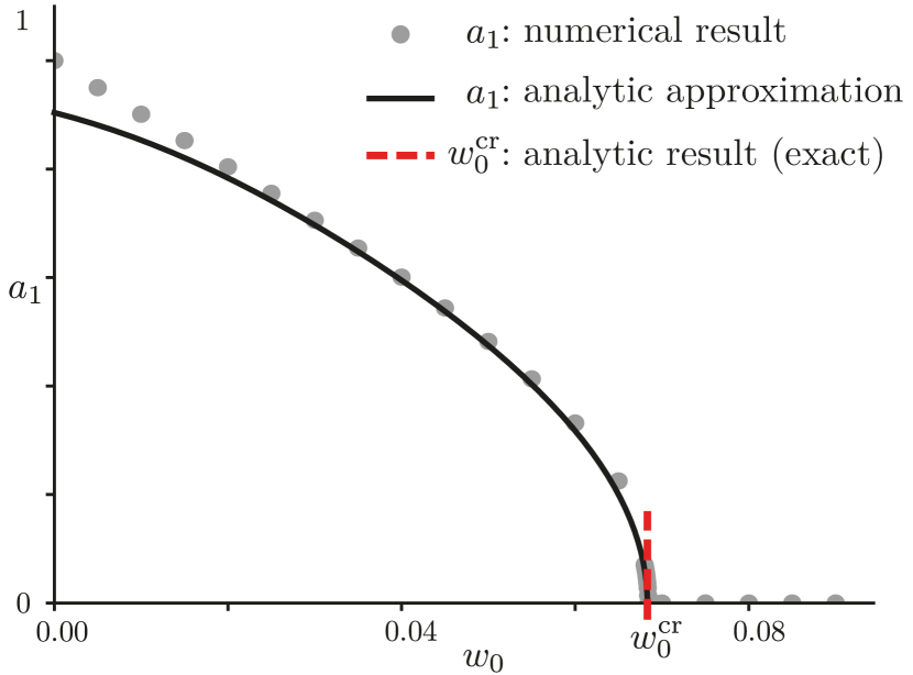
and the scaling behavior of the order parameter close to the critical point . Our analytic approximation of is obtained by closing eq. 8. This procedure provides a generic -th order polynomial for if closed at that order. Thus the best possible analytic solution is a root of a fourth order polynomial, which is plotted in fig. 3 as a solid black line. This solution gets progressively worse away from the critical point, but close to it our numerical and analytic results are in great agreement. Furthermore, we see that this phase transition is unambiguously second order and has a critical exponent of , which was obtained analytically and is exact [19].
For the MCA model we have an additional control parameter , which sets the time scale of the link dynamics. Therefore, we get a critical line
| (10) |
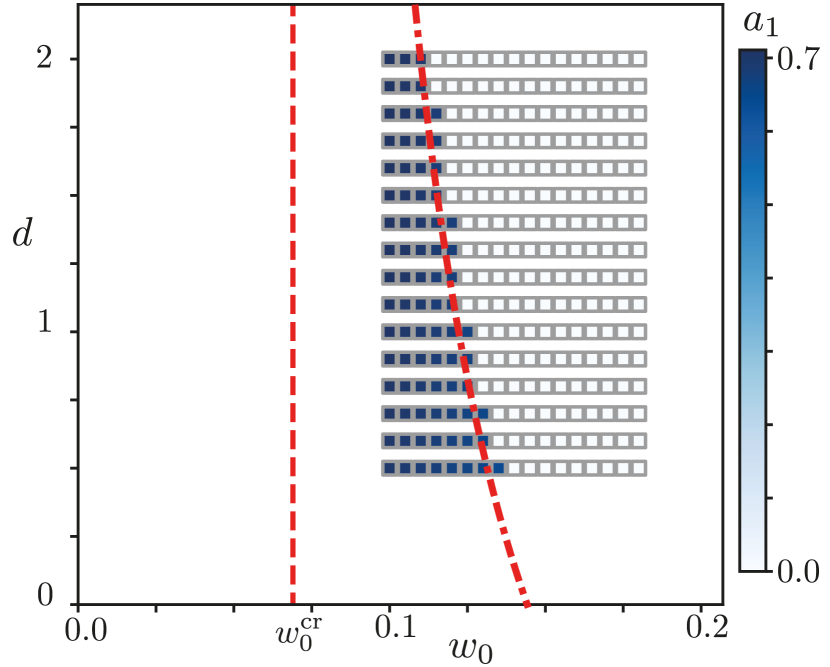
which can be seen in fig. 4, as the red dash-dotted curve. The vertical red dashed line is drawn at the value , this value is reached when goes to infinity. This critical line is obtained by linear stability analysis of the disordered state and is exact, just like the mean field model. The disordered state becomes unstable left of the critical line. Our numerical solutions were obtained by solving the system from an ordered initial condition. Thus the numerical solutions approach the phase transition from the ordered side. The existence of numerical results with nonzero order parameter, on the right of the line indicates hysteresis. Unfortunately, the methods that allowed us to obtain analytic values of the order parameter near criticality in the mean field model do not work here. However the numerical results in fig. 4, clearly show a discontinuous change in the value of the order parameter at the critical line. Together with the bistable region, this is a clear sign of a first order phase transition. To exclude artifacts related to slow convergence to steady state, we repeated the runs for and time steps measured in units of . The results remained unchanged [19].
Discussion –
The continuous state adaptive network model can describe the emergence of swarming. The key parameter in this transition is the relative strength of the noise compared to the agent interactions. The critical noise value, at which the swarming transition occurs, can be changed by tuning the timescale of the network dynamics. However, if this timescale, given by , becomes much smaller than the timescale of the node dynamics, set by , two interesting things happen. First, the region of stability shrinks and the swarming phase transition changes from a first, to a second order transition.
The shrinking of the stable region, for fast link dynamics, is surprising because, the limit of this regime is the mean field approximation. Using the intuition from equilibrium statistical mechanics, one would expect the critical noise to be higher in the case of the mean field model, since we expect mean field models to overestimate the tendency to order. However, we get the opposite result. The critical noise is maximal for ; most likely due to the decoupling of the link dynamics from the state dynamics. This decoupling can slow down the propagation of orientational information through the system.
The second striking effect seen in our system is the meta phase transition. While changing the rate of the link dynamics, the swarming transition becomes second order. Further investigation is necessary, but it seems that this effect can be explained by the observation that the type of noise affects the type of phase transition. According to Pimentel et al. [20] intrinsic noise in agent states leads to a second order transition, while extrinsic noise, caused by imperfect sampling of neighbors, leads to a first order phase transition. This fits well with our findings, since the mean field system only has intrinsic noise caused by spontaneous direction change, while the MCA system introduces an additional noise source, through changing topology. We do not know if this meta transition happens at a finite value of or strictly at , but regardless of the point where the meta transition happens, it constitutes a significant change in the behavior of the system. Biological systems that are described by this model, would therefore not always need nucleation points, such as small co-moving groups, for global swarms to emerge. If such systems could facilitate a quickly changing neighborhood topology, they would be able to smoothly transition into a swarm state.
The new model that we have put forward in this letter demonstrates that the timescale separation between the topology- and state-dynamics of the network has a strong impact on the nature of the swarming transition.
Acknowledgements.
We thank Felix Frey for helpful discussions. G.D. was supported by the “BaSyC – Building a Synthetic Cell” Gravitation grant (024.003.019) of the Netherlands Ministry of Education, Culture and Science (OCW) and the Netherlands Organisation for Scientific Research (NWO).C.K. and G. D. contributed equally to this work.
References
- Vicsek and Zafeiris [2012] T. Vicsek and A. Zafeiris, Physics Reports 517, 71 (2012).
- Bouffanais [2016] R. Bouffanais, Design and Control of Swarm Dynamics, Understanding Complex Systems (Springer Singapore, 2016).
- van Drongelen et al. [2015] R. van Drongelen, A. Pal, C. P. Goodrich, and T. Idema, Physical Review E 91, 032706 (2015).
- McCusker et al. [2019] D. R. McCusker, R. van Drongelen, and T. Idema, EPL (Europhysics Letters) 125, 36001 (2019).
- Echten et al. [2020] D. v. H. t. Echten, G. Nordemann, M. Wehrens, S. Tans, and T. Idema, arXiv:2003.10509 [cond-mat, physics:physics, q-bio] (2020).
- Vicsek et al. [1995] T. Vicsek, A. Czirok, E. Ben-Jacob, I. Cohen, and O. Shochet, Physical Review Letters 75, 1226 (1995).
- Chen et al. [2016] L. Chen, C. Huepe, and T. Gross, Physical Review E 94, 022415 (2016).
- Buhl et al. [2006] J. Buhl, D. J. T. Sumpter, I. D. Couzin, J. J. Hale, E. Despland, E. R. Miller, and S. J. Simpson, Science 312, 1402 (2006).
- Makris et al. [2009] N. C. Makris, P. Ratilal, S. Jagannathan, Z. Gong, M. Andrews, I. Bertsatos, O. R. Godø, R. W. Nero, and J. M. Jech, Science 323, 1734 (2009).
- Huber et al. [2018] L. Huber, R. Suzuki, T. Krüger, E. Frey, and A. R. Bausch, Science 361, 255 (2018).
- Gregoire and Chaté [2004] G. Gregoire and H. Chate, Physical Review Letters 92, 025702 (2004).
- Nagy et al. [2007] M. Nagy, I. Daruka, and T. Vicsek, Physica A: Statistical Mechanics and its Applications 373, 445 (2007).
- Aldana et al. [2007] M. Aldana, V. Dossetti, C. Huepe, V. M. Kenkre, and H. Larralde, Physical Review Letters 98, 095702 (2007).
- Sood and Redner [2005] V. Sood and S. Redner, Physical Review Letters 94, 178701 (2005).
- Huepe et al. [2011] C. Huepe, G. Zschaler, A.-L. Do, and T. Gross, New Journal of Physics 13, 073022 (2011).
- Onsager [1944] L. Onsager, Physical Review 65, 117 (1944).
- Mermin and Wagner [1966] N. D. Mermin and H. Wagner, Physical Review Letters 17, 1133 (1966).
- Merkl and Wagner [1994] F. Merkl and H. Wagner, Journal of Statistical Physics 75, 153 (1994).
- [19] See Supplemental Material at [URL will be inserted by publisher] for derivations and proofs of provided equations.
- Pimentel et al. [2008] J. A. Pimentel, M. Aldana, C. Huepe, and H. Larralde, Physical Review E 77, 061138 (2008).
- [21] Wolfram Research, Inc., Mathematica, Version 12.0, champaign, IL, 2019.
- Rosen [1995] M. I. Rosen, The American Mathematical Monthly 102, 495 (1995).