Emergence of Robust and Efficient Networks
in a Family of Attachment Models

We focus on random and the minimum degree selections of nodes, because they are necessary for generating a strongly robust onion-like networks as follows. In order to make onion-like networks with positive assortativity as degree-degree correlations [16], incrementally growing methods based on a pair of random and intermediation (MED) attachments have been proposed [19, 20]. With either the minimum degree or random selection, the type in MED model is called MED-kmin or MED-rand [20], respectively. In each pair of MED-kmin, one of link destination is chosen uniformly at random (u.a.r), and the other link destination is a node with the minimum degree for intermediation in $\mu$ hops from the randomly chosen pair node. Intermediation in $\mu$ hops means an attachment to a node in the $\mu+1$-th neighbors. Moreover, through numerical simulations, by the iterative attachments to a node at $\mu\geq 3,4$ hops, relatively long loops are formed and enhance the robustness [24]. If the network has a small amount of loops, it can become a tree by removing nodes. Therefore, it is easily fragmented by further attacks to the articular nodes. This phenomenon is supported by the equivalence of dismantling and decycling problems[20]. Similarly in MED-rand, instead of the nodes with the minimum degree, a node is chosen u.a.r in the $\mu+1$-th neighbors from the randomly chosen pair node. Since older nodes with large degrees tend to be selected in the random attachment, this first attachment contributes to enhancing positive correlations among large degree nodes. The other attachment to the nodes with the minimum degree contributes to enhancing positive correlations among small degree nodes. In other words, the second attachment establishes a connection between the minimum degree node in the $\mu+1$-th neighbors and a new node of the minimum degree $m$ in the whole network, therefore it enhances positive correlations among small degree nodes. Note that onion-like networks emerge by MED-kmin, but not by MED-rand [20] because of a weak effect of the second attachment. A modification of MED-kmin will be discussed including the effect of distance regulated by a parameter $\mu$ in Section 3.

In the remaining of this subsection, we show that onion-like networks can also emerge by $k^{-\beta}$-attachment, $0<\beta<\infty$, as an interpolation of random and minimum degree attachments at $\beta=0$ and $\beta\to\infty$. Here, no effect of distance is included in the attachments until the related discussion to MED in Section 3. First, we derive a degree distribution, in which the maximum degree is bounded as $\beta$ becomes larger. Second, for the minimum degree attachment at $\beta\to\infty$, we find that a special chain structure is obtained, the network efficiency is low because of the long distance paths. Third, we numerically investigate three measures: assortativity as degree-degree correlations, robustness of connectivity, and network efficiency in order to reveal which values of $\beta$ contribute to generating both efficient and robust onion-like networks by the $k^{-\beta}$-attachment.

First, as a parametric interpolation between random and minimum degree attachments (at $\beta=0,\infty$), we consider the $k^{-\beta}$-attachment to an existing node $i$ chosen with probability $\frac{k_{i}^{-\beta}}{\sum_{j}k_{j}^{-\beta}}$, $0<\beta<\infty$, for adding $m$ links from a new node at each time step. In general, for a nonlinear attachment to a node $i$ chosen with probability function $f(k_{i})$ of its degree $k_{i}$, the degree distribution $P(k)$ is derived from Eq.(9) in Ref.[14] as follows.

where $K_{\rm min}$ and $K_{\rm max}$ denote the minimum and maximum degrees in a network. In the case of $f(k)=k^{-\beta}$ for $m=K_{\rm min}\leq k\leq K_{\rm max}<\infty$, it is rewritten as,

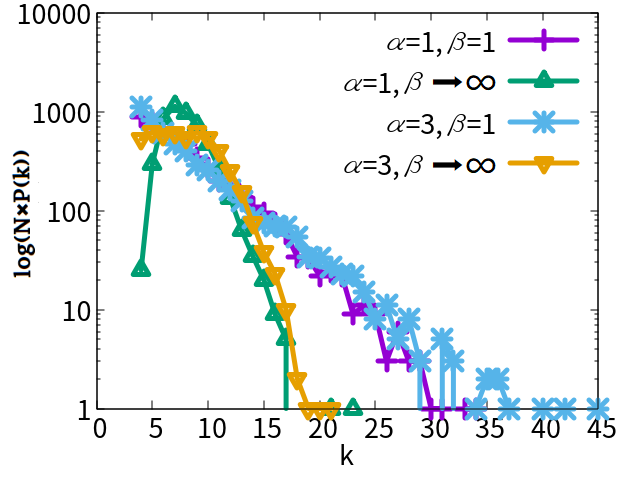
where $C=\mathrm{log}\frac{\langle f\rangle}{\langle f\rangle+m\times f(K_{\rm min})}$ is a constant. In the right-hand side of Eq.(2.2), the constant terms $C$, $\mathrm{log}(m)$, and $\mathrm{log}(\langle f\rangle+m\times K_{\rm min}^{-\beta})>\mathrm{log}(\langle f\rangle+m\times\kappa^{-\beta})$, $K_{\rm min}+1\leq\kappa\leq k$, are not dominant and ignored. Thus, it is approximated as the order of $\mathrm{exp}\left[\int-\beta\mathrm{log}(\kappa)d\kappa\right]\sim e^{-\beta k\mathrm{log}k}$ without the constant factors. Fig. 1 shows a good fitting for the above estimation at $m=2,4$ and $\beta=1,4,10$ by the least squares method for $\mathrm{log}(N\times P(k))$ and $k\mathrm{log}k$. We remark that the maximum degree is decreasing as larger $\beta$ in Fig. 1 and bounded by $2m$ for $\beta\to\infty$ as mentioned later. Note that there is a monotonic increasing relation between $k$ and $k\mathrm{log}k$, $k\geq 1$.

Second, we reveal a special chain structure in the case of $\beta\to\infty$ as the minimum degree attachment. By the attachment at time step $t$, a new node connects to the existing nodes added at $t-1$, $t-2$, …, $t-(m-1)$, whose degree are the smallest $m,...,2m-2$. Because the increase of degree is only one at each time step in prohibiting multi-links. In the total $m$ links, the remaining one link connects to a node with degree $2m-1$ as the next smaller than $2m-2$ because of the minimum degree attachment. Fig. 2 shows a special case of selection to the oldest node with degree $2m-1$ in order to simplify the discussion. While nodes with degree $2m$ do not get a link anymore, since there exists more than one node with degree $2m-1$. We confirm it from the above discussion and Fig. 2 as follows. For the sum $M_{t}$ of degrees at time step $t$, the following equation holds.

where $M_{0}$ and $N_{0}$ are the total numbers of links and nodes in the initial network at $t=0$. $\Delta t$ represents the difference of node IDs defined by the current and the insert time of the oldest node whose degree is less than $2m$. Therefore, $\Delta t$ is not the time duration but the number of nodes. In the right-hand side of Eq.(2.3), $2m(N_{0}+t-\Delta t)$ and $(2m-1)(\Delta t-m)$ denote the sums of degrees of $2m$ and $2m-1$. The third term $\frac{((m+1)+(2m-2+1))(m-1)}{2}$ is the sum of arithmetic sequence from $m+1$ to $2m-2+1$. The last term is the degree $m$ of a new node. We solve Eq.(2.3),

For the initial complete graph, $N_{0}=m+1$ and $M_{0}=\frac{m(m+1)}{2}$ are substituted into Eq.(2.4). Then, we obtain the constant number

From Eq.(2.5), the number of nodes with $2m-1$ is $\Delta t-(m-1)>1$, therefore more than one node with degree $2m-1$ exists.

We remark that the network generated by the minimum degree attachment is an almost regular graph, since many $t-1-\Delta t$ nodes have degree $2m$ after a long time. Moreover, we emphasize that the network has a chain structure with interval of $\Delta t$. In the chain, the longest length of all the shortest paths (the diameter of network) is estimated as $N/\Delta t$. Tables 1 and 2 show that the practical measurement is very close to the estimated value $N/\Delta t$. The slight differences are due to that a node with degree $2m-1$ is randomly selected in the measurement instead of the oldest one in the estimation for a special case of Fig. 2. For $0<\beta<\infty$, the length is longer as $\beta$ increases. Note that the case of $\beta$=0 is random attachment.

To reveal which values of $\beta$ are contributing for generating both efficient and robust onion-like networks by the $k^{-\beta}$-attachment, we investigate the following three measures: assortativity as degree-degree correlations [25, 26], robustness of connectivity [15], and network efficiency [27]. Because the onion-like networks have high assortativity and robustness.

where $S_{1}=\sum_{i}k_{i}$, $S_{2}=\sum_{i}k_{i}^{2}$, $S_{3}=\sum_{i}k_{i}^{3}$, $S_{e}=\sum_{ij}A_{ij}k_{i}k_{j}$, and $A_{ij}$ denotes the $ij$ element of the adjacency matrix. $k_{i}$ and $k_{j}$ denote degrees at end-nodes of $(i,j)$ link. The positive or negative assortativity is distinguished by the sign $r>0$ or $r<0$. $S(Nq)$ denotes the number of nodes included in the giant component (GC as the largest connected cluster) after removing $Nq$ nodes, where $Nq$ is the number of removed nodes by attacks with recalculation of the highest degree node as the target. $1/E$ is the harmonic mean of the shortest path length $L_{ij}$. $L_{ij}$ is counted by the number of hops between nodes $i$ and $j$.

Fig. 3 (a) and (d) show the assortativity for $\beta=0,1,10,50,100$, and $\beta\to\infty$ in the growing networks by the $k^{-\beta}$-attachment. Red line with diamond mark ($\beta\to\infty$) indicates stronger assortativity than purple with cross mark ($\beta=0$), green with square mark ($\beta=1$), cyan with circle mark ($\beta=10$), black with triangle mark ($\beta=50$), and orange with inverse triangle mark ($\beta=100$) lines in Fig. 3 (a) (d). Therefore, the case of larger $\beta$ has higher assortativity. In comparison with the same color lines or marks, the assortativity in Fig. 3 (d) for $m=4$ are higher than that in Fig. 3 (a) for $m=2$. Moreover, as shown in Fig. 3 (b) (e), the robustness in Fig. 3 (e) for $m=4$ are higher than that in Fig. 3 (b) for $m=2$ in comparison with the same color lines or marks. In addition, the lines of assortativity $r$ increase monotonically for varying $\beta$ from 0 to $\infty$ in Fig. 3 (a), while they increase for varying $\beta$ from 0 to 10 in Fig. 3 (b), decrease for varying $\beta$ from 10 to 50, and increase again for varying $\beta$ from 50 to $\infty$. Moreover, the lines of robustness $R$ increase for varying $\beta$ from 0 to 10, decrease for varying $\beta$ from 10 to 50, and increase again for varying $\beta$ from 50 to 100 in Fig. 3 (b) (e). After $\beta$ is greater than 100, the robustness approach to a constant $R$ value. The lines of efficiency $E$ decrease monotonically for varying $\beta$ from 0 to $\infty$ in Fig. 3 (c) (f). The reason why assortativity $r$ and robustness $R$ change in this way is unknown exactly. However, a chain structure may affect them as discussed previously. In particular, red lines at $\beta\to\infty$ in Fig. 3 (d) (e) for $m=4$ show that the network has both high assortativity ($r>0.2$) and robustness ($R>0.3$) as onion-like networks. Note that too strong assortativity lead to rather weaken the robustness with decreasing the value of $R$ [16]. Remember that there are no exact conditions for the values of $r$ and $R$ to be an onion-like network, we consider them as $r>0.2$ and $R>0.3$, because BA model is not an onion-like, which is $r\approx 0$ and $R<0.23$ for the same $N$ and $m$ [19, 20]. Fig. 3 (c) (f) show that the efficiency for $\beta\to\infty$ (red line) becomes lower than ones for $\beta$ = 0, 1, 10, 50, and 100 (purple, green, cyan, black, and orange lines). The reason of low efficiency is due to a chain structure as mentioned in Fig. 2 and Tables 1 and 2.

We investigate the effect of random attachment on the network efficiency whose average lengths are $O(\mathrm{log}N)$ in the mixed attachment of the random attachment and the $k^{-\beta}$-attachment. It is worth to mention that the effect is nontrivial in growing networks, especially by the inverse preferential attachments for a large $\beta$. For example, the diameters are similar as 725.5 and 1000 (365 and 103) obtained by the practice at $\beta=100$ and the estimation for $m=2$ ($m=4$). When $\beta$ is large enough, the diameter becomes $O(N)$ because of approaching to the chain structure. In the following mixed attachment, it is the same that a new node is added at each time step, but the link destinations are chosen by random attachment with probability $p$ and by the $k^{-\beta}$-attachment with probability $1-p$. Note that the case of $\beta=0$ is pure random attachment.

In Fig. 4, green (square mark), brown (pentagon mark), and cyan (circle mark) lines ($\beta=1,4,10$) show that the efficiency trends to increase as the ratio $p$ is larger. We remark that the efficiency rapidly increases for the horizontal axis as shown by black (triangle mark), orange (inverse triangle mark), and red (diamond mark) lines ($\beta=50,100$, and $\beta\to\infty$). This phenomenon corresponds to appearing of chain structures. In comparison with the same color lines or marks, the efficiency in Fig. 4 (b) for $m=4$ are higher than that in Fig. 4 (a) for $m=2$ by using more links in the emergence of onion-like networks. The average length of the shortest paths is given by $\langle L\rangle\approx 1/E$ in a relation of the arithmetic and the harmonic means. For example, the efficiency $E$ = 0.1, 0.2, and 0.25 correspond to the average path lengths of 10, 5, and 4 hops, respectively. Thus, decreasing efficiency $E$ leads to increasing average path length $\langle L\rangle$. As shown in Fig. 5 (a) (c) or (b) (d), the average path length $\langle L\rangle$ decreases in the cases from $p=0$ (top) to $p$ = 0.001, 0.0025, 0.005, 0.05, 0.25, and 0.5 (bottom) denoted by red (asterisk mark), purple (cross mark), green (square mark), cyan (circle mark), orange (triangle mark), black (inverse triangle mark), and blue (diamond mark) lines, respectively. In particular, rapidly increasing (red) curves are obtained for $p=0$ as the pure $k^{-\infty}$-attachment, therefore these results are not proportional to $\mathrm{log}N$ because of the chain structure as mentioned in the previous subsection. However, the exact critical $p_{c}$ is unknown because of a continuous transition of the average path lengths between $O(N)$ and $O(\mathrm{log}N)$. We estimate that it may be between 0.0025 and 0.005 as shown in Fig. 5 (c) (d), in which the average path length becomes longer as almost straight lines of $O(\mathrm{log}N)$ than ones in Fig. 5 (a) (b). In addition, the average path length in Fig. 5 (d) for $m=4$ is shorter than that in Fig. 5 (c) for $m=2$ by using more adding links in comparison with the same color lines or marks. For not only $\beta\to\infty$ but also other values ($\beta=100$), similar results in Fig. 5 are obtained including the critical value: $0.0025\leq p_{c}\leq 0.005$. Thus, a small amount of random attachment is necessary for the emergence of the efficient paths in the mixed attachment.

References

- [1] A.-L. Barabási, R. Albert, Emergence of scaling in random networks, Science 286 (5439) (1999) 509–512. doi:https://doi.org/10.1126/science.286.5439.509.
- [2] R. Albert, H. Jeong, A.-L. Barabási, Error and attack tolerance of complex networks, Nature 406 (6794) (2000) 378–382. doi:https://doi.org/10.1038/35019019.
- [3] A.-L. Barabási, R. Albert, H. Jeong, Mean-field theory for scale-free random networks, Physica A: Statistical Mechanics and its Applications 272 (1-2) (1999) 173–187. doi:https://doi.org/10.1103/PhysRevE.66.055101.
- [4] Z.-G. Shao, X.-W. Zou, Z.-J. Tan, Z.-Z. Jin, Growing networks with mixed attachment mechanisms, Journal of Physics A: Mathematical and General 39 (9) (2006) 2035–2042. doi:https://doi.org/10.1088/0305-4470/39/9/004.
- [5] L. Min, Z. Qinggui, Degree distribution of a mixed attachments model for evolving networks, in: Y. Wu (Ed.), Advanced Technology in Teaching - Proceedings of the 2009 3rd International Conference on Teaching and Computational Science (WTCS 2009), Springer Berlin Heidelberg, Berlin, Heidelberg, 2012, pp. 815–822. doi:https://doi.org/10.1007/978-3-642-25437-6_110.
- [6] P. Holme, B. J. Kim, Growing scale-free networks with tunable clustering, Physical review E 65 (2) (2002) 026107. doi:https://doi.org/10.1103/PhysRevE.65.026107.
- [7] P. L. Krapivsky, S. Redner, F. Leyvraz, Connectivity of growing random networks, Physical Review Letters 85 (21) (2000) 4629. doi:https://doi.org/10.1103/PhysRevLett.85.4629.
- [8] P. L. Krapivsky, S. Redner, Organization of growing random networks, Physical Review E 63 (6) (2001) 066123. doi:https://doi.org/10.1103/PhysRevE.63.066123.
- [9] P. L. Krapivsky, S. Redner, A statistical physics perspective on web growth, Computer Networks 39 (3) (2002) 261–276. doi:https://doi.org/10.1103/PhysRevE.63.066123.
- [10] R. Pastor-Satorras, E. Smith, R. V. Solé, Evolving protein interaction networks through gene duplication, Journal of Theoretical Biology 222 (2) (2003) 199–210. doi:https://doi.org/10.1016/s0022-5193(03)00028-6.
- [11] P. L. Krapivsky, S. Redner, Network growth by copying, Physical Review E 71 (2005) 036118. doi:https://doi.org/10.1103/PhysRevE.71.036118.
- [12] C. S. Q. Siew, M. S. Vitevitch, Investigating the influence of inverse preferential attachment on network development, Entropy 22 (9). doi:10.3390/e22091029.
- [13] C. S. Q. Siew, M. S. Vitevitch, An investigation of network growth principles in the phonological language network, Journal of Experimental Psychology: General 149 (12). doi:10.1037/xge0000876.
- [14] V. Zadorozhnyi, E. Yudin, Growing network: models following nonlinear preferential attachment rule, Physica A: Statistical Mechanics and its Applications 428 (2015) 111–132. doi:https://doi.org/10.1016/j.physa.2015.01.052.
- [15] C. M. Schneider, A. A. Moreira, J. S. Andrade, S. Havlin, H. J. Herrmann, Mitigation of malicious attacks on networks, Proceedings of the National Academy of Sciences 108 (10) (2011) 3838–3841. doi:https://doi.org/10.1073/pnas.1009440108.
- [16] T. Tanizawa, S. Havlin, H. E. Stanley, Robustness of onionlike correlated networks against targeted attacks, Physical. Review. E 85 (2012) 046109. doi:https://doi.org/10.1103/PhysRevE.85.046109.
- [17] Z.-X. Wu, P. Holme, Onion structure and network robustness, Physical Review E 84 (2011) 026106. doi:https://10.1103/PhysRevE.84.026106.
- [18] Y. Hayashi, Growing self-organized design of efficient and robust complex networks, in: 2014 IEEE Eighth International Conference on Self-Adaptive and Self-Organizing Systems, IEEE,Xplore, 2014. doi:https://doi.org/10.1109/SASO.2014.17.
- [19] Y. Hayashi, A new design principle of robust onion-like networks self-organized in growth, Network Science 6 (1) (2018) 54–70. doi:https://doi.org/10.1017/nws.2017.25.
- [20] Y. Hayashi, N. Uchiyama, Onion-like networks are both robust and resilient, Scientific Reports 8 (1) (2018) 1–13. doi:https://doi.org/10.1038/s41598-018-29626-w.
- [21] T. Nishiguchi, A. Beaudet, The toyota group and the aisin fire, Sloan Management Review 40 (1) (1998) 49.
- [22] T. Nishiguchi, A. Beaudet, Fractal design: Self-organizing links in supply chain management, in: Knowledge creation, Springer, 2000, pp. 199–230.
- [23] T. Nishiguchi, Global neighborhoods-strategies of successful organizational networks-(in japanese), NTT Publishing, 2007.
- [24] L. K. Gallos, S. Havlin, H. E. Stanley, N. H. Fefferman, Propinquity drives the emergence of network structure and density, Proceedings of the National Academy of Sciences USA 116 (41) (2019) 20360–20365. doi:https://doi.org/10.1073/pnas.1900219116.
- [25] M. E. Newman, Assortative mixing in networks, Physical Review Letters 89 (20) (2002) 208701. doi:https://doi.org/10.1103/PhysRevLett.89.208701.
- [26] M. Newman, 8.7 Assortative mixing, in: Networks, Oxford University Press, 2010, pp. 266–268.
- [27] V. Latora, M. Marchiori, Efficient behavior of small-world networks, Physical Review Letters 87 (19) (2001) 198701. doi:https://doi.org/10.1103/PhysRevLett.87.198701.
- [28] X.-H. Yang, S.-L. Lou, G. Chen, S.-Y. Chen, W. Huang, Scale-free networks via attaching to random neighbors, Physica A: Statistical Mechanics and its Applications 392 (17) (2013) 3531–3536. doi:https://doi.org/10.1016/j.physa.2013.03.043.