EMCAD: Efficient Multi-scale Convolutional Attention Decoding for Medical Image Segmentation
Abstract
An efficient and effective decoding mechanism is crucial in medical image segmentation, especially in scenarios with limited computational resources. However, these decoding mechanisms usually come with high computational costs. To address this concern, we introduce EMCAD, a new efficient multi-scale convolutional attention decoder, designed to optimize both performance and computational efficiency. EMCAD leverages a unique multi-scale depth-wise convolution block, significantly enhancing feature maps through multi-scale convolutions. EMCAD also employs channel, spatial, and grouped (large-kernel) gated attention mechanisms, which are highly effective at capturing intricate spatial relationships while focusing on salient regions. By employing group and depth-wise convolution, EMCAD is very efficient and scales well (e.g., only 1.91M parameters and 0.381G FLOPs are needed when using a standard encoder). Our rigorous evaluations across 12 datasets that belong to six medical image segmentation tasks reveal that EMCAD achieves state-of-the-art (SOTA) performance with 79.4% and 80.3% reduction in #Params and #FLOPs, respectively. Moreover, EMCAD’s adaptability to different encoders and versatility across segmentation tasks further establish EMCAD as a promising tool, advancing the field towards more efficient and accurate medical image analysis. Our implementation is available at https://github.com/SLDGroup/EMCAD.
1 Introduction
In the realm of medical diagnostics and therapeutic strategies, automated segmentation of medical images is vital, as it classifies pixels to identify critical regions such as lesions, tumors, or entire organs. A variety of U-shaped convolutional neural network (CNN) architectures [44, 41, 62, 24, 20, 37], notably UNet [44], UNet++ [62], UNet3+ [24], and nnU-Net [19], have become standard techniques for this purpose, achieving high-quality, high-resolution segmentation output. Attention mechanisms [41, 12, 20, 57, 17] have also been integrated into these models to enhance feature maps and improve pixel-level classification. Although attention-based models have shown improved performance, they still face significant challenges due to the computationally expensive convolutional blocks that are typically used in conjunction with attention mechanisms.
Recently, vision transformers [18] have shown promise in medical image segmentation tasks [8, 5, 17, 54, 42, 43, 61, 52] by capturing long-range dependencies among pixels through Self-attention (SA) mechanisms. Hierarchical vision transformers like Swin [34], PVT [55, 56], MaxViT [49], MERIT [43], ConvFormer [33], and MetaFormer [59] have been introduced to further improve the performance in this field. While the SA excels at capturing global information, it is less adept at understanding the local spatial context [13, 28]. To address this limitation, some approaches have integrated local convolutional attention within the decoders to better grasp spatial details. Nevertheless, these methods can still be computationally demanding because they frequently employ costly convolutional blocks. This limits their applicability to real-world scenarios where computational resources are restricted.
To address the aforementioned limitations, we introduce EMCAD, an efficient multi-scale convolutional attention decoding using a new multi-scale depth-wise convolution block. More precisely, EMCAD enhances the feature maps via efficient multi-scale convolutions, while incorporating complex spatial relationships and local attention through the use of channel, spatial, and grouped (large-kernel) gated attention mechanisms. Our contributions are as follows:
-
•
New Efficient Multi-scale Convolutional Decoder: We introduce an efficient multi-scale cascaded fully-convolutional attention decoder (EMCAD) for 2D medical image segmentation; this takes the multi-stage features of vision encoders and progressively enhances the multi-scale and multi-resolution spatial representations. EMCAD has only 0.506M parameters and 0.11G FLOPs for a tiny encoder with #channels = [32, 64, 160, 256], while it has 1.91M parameters and 0.381G FLOPs for a standard encoder with #channels = [64, 128, 320, 512].
-
•
Efficient Multi-scale Convolutional Attention Module: We introduce MSCAM, a new efficient multi-scale convolutional attention module that performs depth-wise convolutions at multiple scales; this refines the feature maps produced by vision encoders and enables capturing multi-scale salient features by suppressing irrelevant regions. The use of depth-wise convolutions makes MSCAM very efficient.
-
•
Large-kernel Grouped Attention Gate: We introduce a new grouped attention gate to fuse refined features with the features from skip connections. By using larger kernel () group convolutions instead of point-wise convolutions in the design, we capture salient features in a larger local context with less computation.
-
•
Improved Performance: We empirically show that EMCAD can be used with any hierarchical vision encoder (e.g., PVTv2-B0, PVTv2-B2 [56]), while significantly improving the performance of 2D medical image segmentation. EMCAD produces better results than SOTA methods with a significantly lower computational cost (as shown in Figure 1) on 12 medical image segmentation benchmarks that belong to six different tasks.
The remaining of this paper is organized as follows: Section 2 summarizes related work. Section 3 describes the proposed method. Section 4 explains our experimental setup and results on 12 medical image segmentation benchmarks. Section 5 covers different ablation experiments. Lastly, Section 6 concludes the paper.

2 Related Work
2.1 Vision encoders
Convolutional Neural Networks (CNNs) [32, 46, 21, 47, 22, 45, 23, 48, 35] have been foundational as encoders due to their proficiency in handling spatial relationships in images. More precisely, AlexNet [32] and VGG [46] pave the way, leveraging deep layers of convolutions to extract features progressively. GoogleNet [47] introduces the inception module, allowing more efficient computation of representations across various scales. ResNet [21] introduces residual connections, enabling the training of networks with substantially more layers by addressing the vanishing gradients problem. MobileNets [22, 45] bring CNNs to mobile devices through lightweight, depth-wise separable convolutions. EfficientNet [48] introduces a scalable architectural design to CNNs with compound scaling. Although CNNs are pivotal for many vision applications, they generally lack the ability to capture long-range dependencies within images due to their inherent local receptive fields.
Recently, Vision Transformers (ViTs), pioneered by Dosovitskiy et al. [18], enabled the learning of long-range relationships among pixels using Self-attention (SA). Since then, ViTs have been enhanced by integrating CNN features [56, 49], developing novel self-attention (SA) blocks [34, 49], and introducing new architectural designs [55, 58]. The Swin Transformer [34] incorporates a sliding window attention mechanism, while SegFormer [58] leverages Mix-FFN blocks for hierarchical structures. PVT [55] uses spatial reduction attention, refined in PVTv2 [56] with overlapping patch embedding and a linear complexity attention layer. MaxViT [49] introduces a multi-axis self-attention to form a hierarchical CNN-transformer encoder. Although ViTs address the CNNs limitation in capturing long-range pixel dependencies [32, 46, 21, 47, 22, 45, 23, 48, 35], they face challenges in capturing the local spatial relationships among pixels. In this paper, we aim to overcome these limitations by introducing a new multi-scale cascaded attention decoder that refines feature maps and incorporates local attention using a multi-scale convolutional attention module.
2.2 Medical image segmentation
Medical image segmentation involves pixel-wise classification to identify various anatomical structures like lesions, tumors, or organs within different imaging modalities such as endoscopy, MRI, or CT scans [8]. U-shaped networks [44, 41, 62, 24, 37, 26, 7, 19] are particularly favored due to their simple but effective encoder-decoder design. The UNet [44] pioneered this approach with its use of skip connections to fuse features at different resolution stages. UNet++ [62] evolves this design by incorporating nested encoder-decoder pathways with dense skip connections. Expanding on these ideas, UNet 3+ [24] introduces comprehensive skip pathways that facilitate full-scale feature integration. Further advancement comes with DC-UNet [37], which integrates a multi-resolution convolution scheme and residual paths into its skip connections. The DeepLab series, including DeepLabv3 [10] and DeepLabv3+ [11], introduce atrous convolutions and spatial pyramid pooling to handle multi-scale information. SegNet [2] uses pooling indices to upsample feature maps, preserving the boundary details. nnU-Net [19] automatically configures hyperparameters based on the specific dataset characteristics, using standard 2D and 3D UNets. Collectively, these U-shaped models have become a benchmark for success in the domain of medical image segmentation.
Recently, vision transformers have emerged as a formidable force in medical image segmentation, harnessing the ability to capture pixel relationships at global scales [5, 8, 17, 42, 43, 52, 61, 58]. TransUNet [8] presents a novel blend of CNNs for local feature extraction and transformers for global context, enhancing both local and global feature capture. Swin-Unet [5] extends this by incorporating Swin Transformer blocks [34] into a U-shaped model for both encoding and decoding processes. Building on these concepts, MERIT [43] introduces a multi-scale hierarchical transformer, which employs SA across different window sizes, thus enhancing the model capacity to capture multi-scale features critical for medical image segmentation.
The integration of attention mechanisms has been investigated within CNNs [41, 20] and transformer-based systems [17] for enhancing medical image segmentation. PraNet [20] employs a reverse attention strategy for feature refinement. PolypPVT [17] leverages PVTv2 [56] as its backbone encoder and incorporates CBAM [57] within its decoding stages. The CASCADE [42] presents a novel cascaded decoder, combining channel [23] and spatial [9] attention to refine features at multiple stages, extracted from a transformer encoder, culminating in high-resolution segmentation outputs. While CASCADE achieves notable performance in segmenting medical images by integrating local and global insights from transformers, it is computationally inefficient due to the use of triple convolution layers at each decoder stage. In addition to this, it uses single-scale convolutions during decoding. Our new proposal involves the adoption of multi-scale depth-wise convolutions to mitigate these constraints.
3 Methodology
In this section, we first introduce our new EMCAD decoder and then explain two transformer-based architectures (i.e., PVT-EMCAD-B0 and PVT-EMCAD-B2) incorporating our proposed decoder.

3.1 Efficient multi-scale convolutional attention decoding (EMCAD)
In this section, we introduce our efficient multi-scale convolutional decoding (EMCAD) to process the multi-stage features extracted from pretrained hierarchical vision encoders for high-resolution semantic segmentation. As shown in Figure 2(b), EMCAD consits of efficient multi-scale convolutional attention modules (MSCAMs) to robustly enhance the feature maps, large-kernel grouped attention gates (LGAGs) to refine feature maps fusing with the skip connection via gated attention mechanism, efficient up-convolution blocks (EUCBs) for up-sampling followed by enhancement of feature maps, and segmentation heads (SHs) to produce the segmentation outputs.
More specifically, we use four MSCAMs to refine pyramid features (i.e., , , , in Figure 2) extracted from the four stages of the encoder. After each MSCAM, we use an SH to produce a segmentation map of that stage. Subsequently, we upscale the refined feature maps using EUCBs and add them to the outputs from the corresponding LGAGs. Finally, we add four different segmentation maps to produce the final segmentation output. Different modules of our decoder are described next.
3.1.1 Large-kernel grouped attention gate (LGAG)
We introduce a new large-kernel grouped attention gate (LGAG) to progressively combine feature maps with attention coefficients, which are learned by the network to allow higher activation of relevant features and suppression of irrelevant ones. This process employs a gating signal derived from higher-level features to control the flow of information across different stages of the network, thus enhancing its precision for medical image segmentation. Unlike Attention UNet [41] which uses convolution to process gating signal (features from skip connections) and input feature map (upsampled features), in our (.) function, we process and by applying separate group convolutions (.) and (.), respectively. These convolved features are then normalized using batch normalization ((.)) [27] and merged through element-wise addition. The resultant feature map is activated through a ReLU ((.)) layer [39]. Afterward, we apply a convolution ((.)) followed by (.) layer to get a single channel feature map. We then pass the resultant single-channel feature map through a Sigmoid ((.)) activation function to yield the attention coefficients. The output of this transformation is used to scale the input feature through element-wise multiplication, producing the attention-gated feature . The (·) (Figure 2(g)) can be formulated as in Equations 1 and 2:
| (1) |
| (2) |
Due to using kernel group convolutions in (.), our LGAG captures comparatively larger spatial contexts with less computational cost.
3.1.2 Multi-scale convolutional attention module (MSCAM)
We introduce an efficient multi-scale convolutional attention module to refine the feature maps. MSCAM consists of a channel attention block ((·)) to put emphasis on pertinent channels, a spatial attention block [9] ((·)) to capture the local contextual information, and an efficient multi-scale convolution block ((.)) to enhance the feature maps preserving contextual relationships. The (.) (Figure 2(d)) is given in Equation 3:
| (3) |
where is the input tensor. Due to using depth-wise convolution in multiple scales, our MSCAM is more effective with significantly lower computational cost than the convolutional attention module (CAM) proposed in [42].
Multi-scale Convolution Block (MSCB): We introduce an efficient multi-scale convolution block to enhance the features generated by our cascaded expanding path. In our MSCB, we follow the design of the inverted residual block (IRB) of MobileNetV2 [45]. However, unlike IRB, our MSCB performs depth-wise convolution at multiple scales and uses channel_shuffle [60] to shuffle channels across groups. More specifically, in our MSCB, we first expand the number of channels (i.e., expansion_factor = 2) using a point-wise () convolution layers (·) followed by a batch normalization layer (·) and a ReLU6 [31] activation layer (.). We then use a multi-scale depth-wise convolution (.) to capture both multi-scale and multi-resolution contexts. As depth-wise convolution overlooks the relationships among channels, we use a channel_shuffle operation to incorporate relationships among channels. Afterward, we use another point-wise convolution (.) followed by a (.) to transform back the original #channels, which also encodes dependency among channels. The (·) (Figure 2(e)) is formulated as in Equation 4:
|
|
(4) |
where parallel (.) (Figure 2(f)) for different kernel sizes () can be formulated using Equation 5:
|
|
(5) |
where . Here, (.) is a depth-wise convolution with the kernel size . (.) and (.) are batch normalization and ReLU6 activation, respectively. Additionally, our sequential (.) uses the recursively updated input , where the input is residually connected to the previous (.) for better regularization as in Equation 6:
| (6) |
Channel Attention Block (CAB): We use channel attention block to assign different levels of importance to each channel, thus emphasizing more relevant features while suppressing less useful ones. Basically, the CAB identifies which feature maps to focus on (and then refine them). Following [57], in CAB, we first apply the adaptive maximum pooling ((·)) and adaptive average pooling ((·)) to the spatial dimensions (i.e., height and width) to extract the most significant feature of the entire feature map per channel. Then, for each pooled feature map, we reduce the number of channels times separately using a point-wise convolution ((·)) followed by a ReLU activation (). Afterward, we recover the original channels using another point-wise convolution ((·)). We then add both recovered feature maps and apply Sigmoid () activation to estimate attention weights. Finally, we incorporate these weights to input using the Hadamard product (). The (·) (Figure 2(h)) is defined using Equation 7:
|
|
(7) |
Spatial Attention Block (SAB): We use spatial attention to mimic the attentional processes of the human brain by focusing on specific parts of an input image. Basically, the SAB determines where to focus in a feature map; then it enhances those features. This process enhances the model’s ability to recognize and respond to relevant spatial features, which is crucial for image segmentation where the context and location of objects significantly influence the output. In SAB, we first pool maximum ((·)) and average ((·)) values along the channel dimension to pay attention to local features. Then, we use a large kernel (i.e., as in [17]) convolution layer to enhance local contextual relationships among features. Afterward, we apply the Sigmoid activation () to calculate attention weights. Finally, we feed these weights to the input (using Hadamard product () to attend information in a more targeted way. The (.) (Figure 2(i)) is defined using Equation 8:
| (8) |
3.1.3 Efficient up-convolution block (EUCB)
We use an efficient up-convolution block to progressively upsample the feature maps of the current stage to match the dimension and resolution of the feature maps from the next skip connection. The EUCB first uses an UpSampling (·) with scale-factor 2 to upscale the feature maps. Then, it enhances the upscaled feature maps by applying a depth-wise convolution (·) followed by a (·) and a (.) activation. Finally, a convolution (.) is used to reduce the #channels to match with the next stage. The (·) (Figure 2(c)) is formulated as in Equation 9:
| (9) |
Due to using depth-wise convolution instead of convolution, our EUCB is very efficient.
3.1.4 Segmentation head (SH)
We use segmentation heads to produce the segmentation outputs from the refined feature maps of four stages of the decoder. The SH layer applies a convolution (·) to the refined feature maps having channels ( is the #channels in the feature map of stage ) and produces output with #channels equal to #classes in target dataset for multi-class but channel for binary segmentation. The (·) is formulated as in Equation 10:
| (10) |
3.2 Overall architecture
To show the generalization, effectiveness, and ability to process multi-scale features for medical image segmentation, we integrate our EMCAD decoder alongside tiny (PVTv2-B0) and standard (PVTv2-B2) networks of PVTv2 [56]. However, our decoder is adaptable and seamlessly compatible with other hierarchical backbone networks.
PVTv2 differs from conventional transformer patch embedding modules by applying convolutional operations for consistent spatial information capture. Using PVTv2-b0 (Tiny) and PVTv2-b2 (Standard) encoders [56], we develop the PVT-EMCAD-B0 and PVT-EMCAD-B2 architectures. To adopt PVTv2, we first extract the features (X1, X2, X3, and X4) from four layers and feed them (i.e., X4 in the upsample path and X3, X2, X1 in the skip connections) into our EMCAD decoder as shown in Figure 2(a-b). EMCAD then processes them and produces four segmentation maps that correspond to the four stages of the encoder network.
3.3 Multi-stage loss and outputs aggregation
Our EMCAD decoder’s four segmentation heads produce four prediction maps , , , and across its stages.
Loss aggregation: We adopt a combinatorial approach to loss combination called MUTATION, inspired by the work of MERIT [43] for multi-class segmentation. This involves calculating the loss for all possible combinations of predictions derived from heads, totaling unique predictions, and then summing these losses. We focus on minimizing this cumulative combinatorial loss during the training process. For binary segmentation, we optimize the additive loss like [42] with an additional term as in Equation 11:
|
|
(11) |
where , , , and are the losses of each individual prediction maps. are the weights assigned to each loss.
Output segmentation maps aggregation: We consider the prediction map, , from the last stage of our decoder as the final segmentation map. Then, we obtain the final segmentation output by employing a function for binary or a function for multi-class segmentation.
4 Experiments

Methods #Params #FLOPs Polyp Skin Lesion Cell BUSI Avg. Clinic Colon ETIS Kvasir BKAI ISIC17 ISIC18 DSB18 EM UNet [44] 34.53M 65.53G 92.11 83.95 76.85 82.87 85.05 83.07 86.67 92.23 95.46 74.04 85.23 UNet++ [62] 9.16M 34.65G 92.17 87.88 77.40 83.36 84.07 82.98 87.46 91.97 95.48 74.76 85.75 AttnUNet [41] 34.88M 66.64G 92.20 86.46 76.84 83.49 84.07 83.66 87.05 92.22 95.55 74.48 85.60 DeepLabv3+ [10] 39.76M 14.92G 93.24 91.92 90.73 89.06 89.74 83.84 88.64 92.14 94.96 76.81 89.11 PraNet [20] 32.55M 6.93G 91.71 89.16 83.84 84.82 85.56 83.03 88.56 89.89 92.37 75.14 86.41 CaraNet [38] 46.64M 11.48G 94.08 91.19 90.25 89.74 89.71 85.02 90.18 89.15 92.78 77.34 88.94 UACANet-L [30] 69.16M 31.51G 94.16 91.02 89.77 90.17 90.35 83.72 89.76 88.86 89.28 76.96 88.41 SSFormer-L [54] 66.22M 17.28G 94.18 92.11 90.16 91.47 91.14 85.28 90.25 92.03 94.95 78.76 90.03 PolypPVT [17] 25.11M 5.30G 94.13 91.53 89.93 91.56 91.17 85.56 90.36 90.69 94.40 79.35 89.87 TransUNet [8] 105.32M 38.52G 93.90 91.63 87.79 91.08 89.17 85.00 89.16 92.04 95.27 78.30 89.33 SwinUNet [5] 27.17M 6.2G 92.42 89.27 85.10 89.59 87.61 83.97 89.26 91.03 94.47 77.38 88.01 TransFuse [61] 143.74M 82.71G 93.62 90.35 86.91 90.24 87.47 84.89 89.62 90.85 94.35 79.36 88.77 UNeXt [50] 1.47M 0.57G 90.20 83.84 74.03 77.88 77.93 82.74 87.78 86.01 93.81 74.71 82.89 PVT-CASCADE [42] 34.12M 7.62G 94.53 91.60 91.03 92.05 92.14 85.50 90.41 92.35 95.42 79.21 90.42 PVT-EMCAD-B0 (Ours) 3.92M 0.84G 94.60 91.71 91.65 91.95 91.30 85.67 90.70 92.46 95.35 79.80 90.52 PVT-EMCAD-B2 (Ours) 26.76M 5.6G 95.21 92.31 92.29 92.75 92.96 85.95 90.96 92.74 95.53 80.25 91.10
| Architectures | Average | Aorta | GB | KL | KR | Liver | PC | SP | SM | ||
|---|---|---|---|---|---|---|---|---|---|---|---|
| DICE | HD95 | mIoU | |||||||||
| UNet [44] | 70.11 | 44.69 | 59.39 | 84.00 | 56.70 | 72.41 | 62.64 | 86.98 | 48.73 | 81.48 | 67.96 |
| AttnUNet [41] | 71.70 | 34.47 | 61.38 | 82.61 | 61.94 | 76.07 | 70.42 | 87.54 | 46.70 | 80.67 | 67.66 |
| R50+UNet [8] | 74.68 | 36.87 | 84.18 | 62.84 | 79.19 | 71.29 | 93.35 | 48.23 | 84.41 | 73.92 | |
| R50+AttnUNet [8] | 75.57 | 36.97 | 55.92 | 63.91 | 79.20 | 72.71 | 93.56 | 49.37 | 87.19 | 74.95 | |
| SSFormer [54] | 78.01 | 25.72 | 67.23 | 82.78 | 63.74 | 80.72 | 78.11 | 93.53 | 61.53 | 87.07 | 76.61 |
| PolypPVT [17] | 78.08 | 25.61 | 67.43 | 82.34 | 66.14 | 81.21 | 73.78 | 94.37 | 59.34 | 88.05 | 79.4 |
| TransUNet [8] | 77.61 | 26.9 | 67.32 | 86.56 | 60.43 | 80.54 | 78.53 | 94.33 | 58.47 | 87.06 | 75.00 |
| SwinUNet [5] | 77.58 | 27.32 | 66.88 | 81.76 | 65.95 | 82.32 | 79.22 | 93.73 | 53.81 | 88.04 | 75.79 |
| MT-UNet [53] | 78.59 | 26.59 | 87.92 | 64.99 | 81.47 | 77.29 | 93.06 | 59.46 | 87.75 | 76.81 | |
| MISSFormer [25] | 81.96 | 18.20 | 86.99 | 68.65 | 85.21 | 82.00 | 94.41 | 65.67 | 91.92 | 80.81 | |
| PVT-CASCADE [42] | 81.06 | 20.23 | 70.88 | 83.01 | 70.59 | 82.23 | 80.37 | 94.08 | 64.43 | 90.1 | 83.69 |
| TransCASCADE [42] | 82.68 | 17.34 | 73.48 | 86.63 | 68.48 | 87.66 | 84.56 | 94.43 | 65.33 | 90.79 | 83.52 |
| PVT-EMCAD-B0 (Ours) | 81.97 | 17.39 | 72.64 | 87.21 | 66.62 | 87.48 | 83.96 | 94.57 | 62.00 | 92.66 | 81.22 |
| PVT-EMCAD-B2 (Ours) | 83.63 | 15.68 | 74.65 | 88.14 | 68.87 | 88.08 | 84.10 | 95.26 | 68.51 | 92.17 | 83.92 |
In this section, we present the details of our implementation followed by a comparative analysis of our PVT-EMCAD-B0 and PVT-EMCAD-B2 against SOTA methods. Datasets and evaluation metrics are in Supplementary Section 7.
Methods Avg. DICE RV Myo LV R50+UNet [8] 87.55 87.10 80.63 94.92 R50+AttnUNet [8] 86.75 87.58 79.20 93.47 ViT+CUP [8] 81.45 81.46 70.71 92.18 R50+ViT+CUP [8] 87.57 86.07 81.88 94.75 TransUNet [8] 89.71 86.67 87.27 95.18 SwinUNet [5] 88.07 85.77 84.42 94.03 MT-UNet [53] 90.43 86.64 89.04 95.62 MISSFormer [25] 90.86 89.55 88.04 94.99 PVT-CASCADE [42] 91.46 89.97 88.9 95.50 TransCASCADE [42] 91.63 90.25 89.14 95.50 Cascaded MERIT [43] 91.85 90.23 89.53 95.80 PVT-EMCAD-B0 (Ours) 91.34 89.37 88.99 95.65 PVT-EMCAD-B2 (Ours) 92.12 90.65 89.68 96.02
4.1 Implementation details
We implement our network and conduct experiments using Pytorch 1.11.0 on a single NVIDIA RTX A6000 GPU with 48GB of memory. We utilize ImageNet [16] pre-trained PVTv2-b0 and PVTv2-b2 [56] as encoders. In the MSDC of our decoder, we set the multi-scale kernels through an ablation study. We use the parallel arrangement of depth-wise convolutions in all experiments. Our models are trained using the AdamW optimizer [36] with a learning rate and weight decay of . We generally train for 200 epochs with a batch size of 16, except for Synapse multi-organ (300 epochs, batch size 6) and ACDC cardiac organ (400 epochs, batch size 12), saving the best model based on the DICE score. We resize images to and use a multi-scale {0.75, 1.0, 1.25} training strategy with a gradient clip limit of 0.5 for ClinicDB [3], Kvasir [29], ColonDB [51], ETIS [51], BKAI [40], ISIC17 [15], and ISIC18 [15], while we resize images to for BUSI [1], EM [6], and DSB18 [4]. For Synapse and ACDC datasets, images are resized to , with random rotation and flipping augmentations, optimizing a combined Cross-entropy (0.3) and DICE (0.7) loss. For binary segmentation, we utilize the combined weighted BinaryCrossEntropy (BCE) and weighted IoU loss function.
4.2 Results
We compare our architectures (i.e., PVT-EMCAD-B0 and PVT-EMCAD-B2) with SOTA CNN and transformer-based segmentation methods on 12 datasets that belong to six medical image segmentation tasks. Qualitative results are in the Supplementary Section 7.3.
4.2.1 Results of binary medical image segmentation
Results for different methods on 10 binary medical image segmentation datasets are shown in Table 1 and Figure 1. Our PVT-EMCAD-B2 attains the highest average DICE score (91.10%) with only 26.76M parameters and 5.6G FLOPs. The multi-scale depth-wise convolution in our EMCAD decoder, combined with the transformer encoder, contributes to these performance gains.
Polyp segmentation: Table 1 reveals that our PVT-EMCAD-B2 surpasses all SOTA methods in five polyp segmentation datasets. PVT-EMCAD-B2 achieves DICE score improvements of 1.08%, 0.78%, 2.36%, 1.19%, and 1.79% over PolypPVT in ClinicDB, ColonDB, ETIS, Kvasir, and BKAI-IGI, despite having slightly more parameters and FLOPs. The smallest model UNeXt, exhibits the worst performance in all five polyp segmentation datasets. Our smaller model with only 3.92M parameters and 0.84G FLOPs also outperforms all the methods except PVT-CASCADE (in Kvasir and BKAI-IGH) and SSFormer-L (in ColonDB), which achieve the best performance among SOTA methods. In conclusion, our PVT-EMCAD-B2 achieves the new SOTA results in these five polyp segmentation datasets.
Skin lesion segmentation: Table 1 shows PVT-EMCAD-B2’s strong performance on ISIC17 and ISIC18 skin lesion segmentation datasets, achieving DICE scores of 85.95% and 90.96%, surpassing DeepLabV3+ by 2.11% and 2.32%. It also beats the nearest method PVT-CASCADE by 0.45% and 0.55% in ISIC17 and ISIC18, respectively, though our decoder is significantly more efficient than CASCADE. Our PVT-EMCAD-B0 also shows huge potential in point care applications like skin lesion segmentation with only 3.92M parameters and 0.84G FLOPs.
Cell segmentation: To evaluate our method’s effectiveness in biological imaging, we use DSB18 [4] for cell nuclei and EM [6] for cell structure segmentation. As Table 1 indicates, our PVT-EMCAD-B2 sets a SOTA benchmark in cell nuclei segmentation on DSB18, outperforming DeepLabv3+, TransFuse, and PVT-CASCADE. On the EM dataset, PVT-EMCAD-B2 secures the second-best DICE score (95.53%), offering significantly lower computational costs than the top-performing AttnUNet (95.55%).
Breast cancer segmentation: We conduct experiments on the BUSI dataset for breast cancer segmentation in ultrasound images. Our PVT-EMCAD-B2 achieves the SOTA DICE score (80.25%) on this dataset. Furthermore, our PVT-EMCAD-B0 outperforms the computationally similar method UNeXt by a notable margin of 5.54%.
Components #FLOPs(G) #Params Avg Cascaded LGAG MSCAM 224 256 (M) DICE No No No 0 0 0 80.100.2 Yes No No 0.100 0.131 0.224 81.080.2 Yes Yes No 0.108 0.141 0.235 81.920.2 Yes No Yes 0.373 0.487 1.898 82.860.3 Yes Yes Yes 0.381 0.498 1.91 83.630.3
Conv. kernels Synapse 82.43 82.79 82.74 82.98 82.81 83.63 82.92 83.11 83.57 83.34 ClinicDB 94.81 94.90 94.98 95.13 95.06 95.21 95.15 95.03 95.18 95.07
4.2.2 Results of abdomen organ segmentation
Table 2 shows that our PVT-EMCAD-B2 excels in abdomen organ segmentation on the Synapse multi-organ dataset, achieving the highest average DICE score of 83.63% and surpassing all SOTA CNN- and transformer-based methods. It outperforms PVT-CASCADE by 2.57% in DICE score and 4.55 in HD95 distance, indicating superior organ boundary location. Our EMCAD decoder boosts individual organ segmentation, significantly outperforming SOTA methods on six of eight organs.
4.2.3 Results of cardiac organ segmentation
Table 3 shows the DICE scores of our PVT-EMCAD-B2 and PVT-EMCAD-B0 along with other SOTA methods, on the MRI images of the ACDC dataset for cardiac organ segmentation. Our PVT-EMCAD-B2 achieves the highest average DICE score of 92.12%, thus improving about 0.27% over Cascaded MERIT though our network has significantly lower computational cost. Besides, PVT-EMCAD-B2 has better DICE scores in all three organ segmentations.
5 Ablation Studies
Encoders Decoders #FLOPs(G) #Params(M) DICE (%) PVTv2-B0 CASCADE 0.439 2.32 80.54 PVTv2-B0 EMCAD (Ours) 0.110 0.507 81.97 PVTv2-B2 CASCADE 1.93 9.27 82.78 PVTv2-B2 EMCAD (Ours) 0.381 1.91 83.63
In this section, we conduct ablation studies to explore different aspects of our architectures and the experimental framework. More ablations are in Supplementary Section 8.
5.1 Effect of different components of EMCAD
We conduct a set of experiments on the Synapse multi-organ dataset to understand the effect of different components of our EMCAD decoder. We start with only the encoder and add different modules such as Cascaded structure, LGAG, and MSCAM to understand their effect. Table 4 exhibits that the cascaded structure of the decoder helps to improve performance over the non-cascaded one. The incorporation of LGAG and MSCAM improves performance, however, MSCAM proves to be more effective. When both the LGAG and MSCAM modules are used together, it produces the best DICE score of 83.63%. It is also evident that there is about 3.53% improvement in the DICE score with an additional 0.381G FLOPs and 1.91M parameters.
5.2 Effect of multi-scale kernels in MSCAM
We have conducted another set of experiments on Synapse multi-organ and ClinicDB datasets to understand the effect of different multi-scale kernels used for depth-wise convolutions in MSDC. Table 5 reports these results which show that performance improves from to kernel. When kernel is used together with it improves more than when using them alone. However, when two kernels are used together, performance drops. The incorporation of a kernel with and kernels further improves the performance and it achieves the best results in both Synapse multi-organ and ClinicDB datasets. If we add additional larger kernels (e.g., , ), the performance of both datasets drops. Based on these empirical observations, we choose kernels in all our experiments.
5.3 Comparison with the baseline decoder
In Table 6, we report the experimental results with the computational complexity of our EMCAD decoder and a baseline decoder, namely CASCADE. From Table 6, we can see that our EMCAD decoder with PVTv2-b2 requires 80.3% fewer FLOPs and 79.4% fewer parameters to outperform (by 0.85%) the respective CASCADE decoder. Similarly, our EMCAD decoder with PVTv2-B0 achieves 1.43% better DICE score than the CASCADE decoder with 78.1% fewer parameters and 74.9% fewer FLOPs.
6 Conclusions
In this paper, we have presented EMCAD, a new and efficient multi-scale convolutional attention decoder designed for multi-stage feature aggregation and refinement in medical image segmentation. EMCAD employs a multi-scale depth-wise convolution block, which is key for capturing diverse scale information within feature maps, a critical factor for precision in medical image segmentation. This design choice, using depth-wise convolutions instead of standard convolution blocks, makes EMCAD notably efficient.
Our experiments reveal that EMCAD surpasses the recent CASCADE decoder in DICE scores with 79.4% fewer parameters and 80.3% less FLOPs. Our extensive experiments also confirm EMCAD’s superior performance compared to SOTA methods across 12 public datasets covering six different 2D medical image segmentation tasks. EMCAD’s compatibility with smaller encoders makes it an excellent fit for point-of-care applications while maintaining high performance. We anticipate that our EMCAD decoder will be a valuable asset in enhancing a variety of medical image segmentation and semantic segmentation tasks.
Acknowledgements: This work is supported in part by the NSF grant CNS 2007284, and in part by the iMAGiNE Consortium (https://imagine.utexas.edu/).
References
- Al-Dhabyani et al. [2020] Walid Al-Dhabyani, Mohammed Gomaa, Hussien Khaled, and Aly Fahmy. Dataset of breast ultrasound images. Data in brief, 28:104863, 2020.
- Badrinarayanan et al. [2017] Vijay Badrinarayanan, Alex Kendall, and Roberto Cipolla. Segnet: A deep convolutional encoder-decoder architecture for image segmentation. IEEE Trans. Pattern Anal. Mach. Intell., 39(12):2481–2495, 2017.
- Bernal et al. [2015] Jorge Bernal, F Javier Sánchez, Gloria Fernández-Esparrach, Debora Gil, Cristina Rodríguez, and Fernando Vilariño. Wm-dova maps for accurate polyp highlighting in colonoscopy: Validation vs. saliency maps from physicians. Comput. Med. Imaging Graph., 43:99–111, 2015.
- Caicedo et al. [2019] Juan C Caicedo, Allen Goodman, Kyle W Karhohs, Beth A Cimini, Jeanelle Ackerman, Marzieh Haghighi, CherKeng Heng, Tim Becker, Minh Doan, Claire McQuin, et al. Nucleus segmentation across imaging experiments: the 2018 data science bowl. Nature methods, 16(12):1247–1253, 2019.
- Cao et al. [2021] Hu Cao, Yueyue Wang, Joy Chen, Dongsheng Jiang, Xiaopeng Zhang, Qi Tian, and Manning Wang. Swin-unet: Unet-like pure transformer for medical image segmentation. arXiv preprint arXiv:2105.05537, 2021.
- Cardona et al. [2010] Albert Cardona, Stephan Saalfeld, Stephan Preibisch, Benjamin Schmid, Anchi Cheng, Jim Pulokas, Pavel Tomancak, and Volker Hartenstein. An integrated micro-and macroarchitectural analysis of the drosophila brain by computer-assisted serial section electron microscopy. PLoS biology, 8(10):e1000502, 2010.
- Chen et al. [2022] Gongping Chen, Lei Li, Yu Dai, Jianxun Zhang, and Moi Hoon Yap. Aau-net: an adaptive attention u-net for breast lesions segmentation in ultrasound images. IEEE Trans. Med. Imaging, 2022.
- Chen et al. [2021] Jieneng Chen, Yongyi Lu, Qihang Yu, Xiangde Luo, Ehsan Adeli, Yan Wang, Le Lu, Alan L Yuille, and Yuyin Zhou. Transunet: Transformers make strong encoders for medical image segmentation. arXiv preprint arXiv:2102.04306, 2021.
- Chen et al. [2017a] Long Chen, Hanwang Zhang, Jun Xiao, Liqiang Nie, Jian Shao, Wei Liu, and Tat-Seng Chua. Sca-cnn: Spatial and channel-wise attention in convolutional networks for image captioning. In IEEE Conf. Comput. Vis. Pattern Recog., pages 5659–5667, 2017a.
- Chen et al. [2017b] Liang-Chieh Chen, George Papandreou, Iasonas Kokkinos, Kevin Murphy, and Alan L Yuille. Deeplab: Semantic image segmentation with deep convolutional nets, atrous convolution, and fully connected crfs. IEEE Trans. Pattern Anal. Mach. Intell., 40(4):834–848, 2017b.
- Chen et al. [2018a] Liang-Chieh Chen, Yukun Zhu, George Papandreou, Florian Schroff, and Hartwig Adam. Encoder-decoder with atrous separable convolution for semantic image segmentation. In Eur. Conf. Comput. Vis., pages 801–818, 2018a.
- Chen et al. [2018b] Shuhan Chen, Xiuli Tan, Ben Wang, and Xuelong Hu. Reverse attention for salient object detection. In Eur. Conf. Comput. Vis., pages 234–250, 2018b.
- Chu et al. [2021] Xiangxiang Chu, Zhi Tian, Bo Zhang, Xinlong Wang, Xiaolin Wei, Huaxia Xia, and Chunhua Shen. Conditional positional encodings for vision transformers. arXiv preprint arXiv:2102.10882, 2021.
- Codella et al. [2019] Noel Codella, Veronica Rotemberg, Philipp Tschandl, M Emre Celebi, Stephen Dusza, David Gutman, Brian Helba, Aadi Kalloo, Konstantinos Liopyris, Michael Marchetti, et al. Skin lesion analysis toward melanoma detection 2018: A challenge hosted by the international skin imaging collaboration (isic). arXiv preprint arXiv:1902.03368, 2019.
- Codella et al. [2018] Noel CF Codella, David Gutman, M Emre Celebi, Brian Helba, Michael A Marchetti, Stephen W Dusza, Aadi Kalloo, Konstantinos Liopyris, Nabin Mishra, Harald Kittler, et al. Skin lesion analysis toward melanoma detection: A challenge at the 2017 international symposium on biomedical imaging (isbi), hosted by the international skin imaging collaboration (isic). In IEEE Int. Symp. Biomed. Imaging, pages 168–172. IEEE, 2018.
- Deng et al. [2009] Jia Deng, Wei Dong, Richard Socher, Li-Jia Li, Kai Li, and Li Fei-Fei. Imagenet: A large-scale hierarchical image database. In IEEE Conf. Comput. Vis. Pattern Recog., pages 248–255. Ieee, 2009.
- Dong et al. [2021] Bo Dong, Wenhai Wang, Deng-Ping Fan, Jinpeng Li, Huazhu Fu, and Ling Shao. Polyp-pvt: Polyp segmentation with pyramid vision transformers. arXiv preprint arXiv:2108.06932, 2021.
- Dosovitskiy et al. [2020] Alexey Dosovitskiy, Lucas Beyer, Alexander Kolesnikov, Dirk Weissenborn, Xiaohua Zhai, Thomas Unterthiner, Mostafa Dehghani, Matthias Minderer, Georg Heigold, Sylvain Gelly, et al. An image is worth 16x16 words: Transformers for image recognition at scale. arXiv preprint arXiv:2010.11929, 2020.
- et al. [2021] Isensee et al. nnu-net: a self-configuring method for deep learning-based biomedical image segmentation. Nature methods, 18(2):203–211, 2021.
- Fan et al. [2020] Deng-Ping Fan, Ge-Peng Ji, Tao Zhou, Geng Chen, Huazhu Fu, Jianbing Shen, and Ling Shao. Pranet: Parallel reverse attention network for polyp segmentation. In Int. Conf. Med. Image Comput. Comput. Assist. Interv., pages 263–273. Springer, 2020.
- He et al. [2016] Kaiming He, Xiangyu Zhang, Shaoqing Ren, and Jian Sun. Deep residual learning for image recognition. In IEEE Conf. Comput. Vis. Pattern Recog., pages 770–778, 2016.
- Howard et al. [2017] Andrew G Howard, Menglong Zhu, Bo Chen, Dmitry Kalenichenko, Weijun Wang, Tobias Weyand, Marco Andreetto, and Hartwig Adam. Mobilenets: Efficient convolutional neural networks for mobile vision applications. arXiv preprint arXiv:1704.04861, 2017.
- Hu et al. [2018] Jie Hu, Li Shen, and Gang Sun. Squeeze-and-excitation networks. In IEEE Conf. Comput. Vis. Pattern Recog., pages 7132–7141, 2018.
- Huang et al. [2020] Huimin Huang, Lanfen Lin, Ruofeng Tong, Hongjie Hu, Qiaowei Zhang, Yutaro Iwamoto, Xianhua Han, Yen-Wei Chen, and Jian Wu. Unet 3+: A full-scale connected unet for medical image segmentation. In ICASSP, pages 1055–1059. IEEE, 2020.
- Huang et al. [2021] Xiaohong Huang, Zhifang Deng, Dandan Li, and Xueguang Yuan. Missformer: An effective medical image segmentation transformer. arXiv preprint arXiv:2109.07162, 2021.
- Ibtehaz and Kihara [2023] Nabil Ibtehaz and Daisuke Kihara. Acc-unet: A completely convolutional unet model for the 2020s. In Int. Conf. Med. Image Comput. Comput. Assist. Interv., pages 692–702. Springer, 2023.
- Ioffe and Szegedy [2015] Sergey Ioffe and Christian Szegedy. Batch normalization: Accelerating deep network training by reducing internal covariate shift. In Int. Conf. Mach. Learn., pages 448–456. pmlr, 2015.
- Islam et al. [2020] Md Amirul Islam, Sen Jia, and Neil DB Bruce. How much position information do convolutional neural networks encode? arXiv preprint arXiv:2001.08248, 2020.
- Jha et al. [2020] Debesh Jha, Pia H Smedsrud, Michael A Riegler, Pål Halvorsen, Thomas de Lange, Dag Johansen, and Håvard D Johansen. Kvasir-seg: A segmented polyp dataset. In Int. Conf. Multimedia Model., pages 451–462. Springer, 2020.
- Kim et al. [2021] Taehun Kim, Hyemin Lee, and Daijin Kim. Uacanet: Uncertainty augmented context attention for polyp segmentation. In ACM Int. Conf. Multimedia, pages 2167–2175, 2021.
- Krizhevsky and Hinton [2010] Alex Krizhevsky and Geoff Hinton. Convolutional deep belief networks on cifar-10. Unpublished manuscript, 40(7):1–9, 2010.
- Krizhevsky et al. [2012] Alex Krizhevsky, Ilya Sutskever, and Geoffrey E Hinton. Imagenet classification with deep convolutional neural networks. Adv. Neural Inform. Process. Syst., 25, 2012.
- Lin et al. [2023] Xian Lin, Zengqiang Yan, Xianbo Deng, Chuansheng Zheng, and Li Yu. Convformer: Plug-and-play cnn-style transformers for improving medical image segmentation. In Int. Conf. Med. Image Comput. Comput. Assist. Interv., pages 642–651. Springer, 2023.
- Liu et al. [2021] Ze Liu, Yutong Lin, Yue Cao, Han Hu, Yixuan Wei, Zheng Zhang, Stephen Lin, and Baining Guo. Swin transformer: Hierarchical vision transformer using shifted windows. In Int. Conf. Comput. Vis., pages 10012–10022, 2021.
- Liu et al. [2022] Zhuang Liu, Hanzi Mao, Chao-Yuan Wu, Christoph Feichtenhofer, Trevor Darrell, and Saining Xie. A convnet for the 2020s. In IEEE Conf. Comput. Vis. Pattern Recog., pages 11976–11986, 2022.
- Loshchilov and Hutter [2017] Ilya Loshchilov and Frank Hutter. Decoupled weight decay regularization. arXiv preprint arXiv:1711.05101, 2017.
- Lou et al. [2021] Ange Lou, Shuyue Guan, and Murray Loew. Dc-unet: rethinking the u-net architecture with dual channel efficient cnn for medical image segmentation. In Med. Imaging 2021: Image Process., pages 758–768. SPIE, 2021.
- Lou et al. [2022] Ange Lou, Shuyue Guan, Hanseok Ko, and Murray H Loew. Caranet: context axial reverse attention network for segmentation of small medical objects. In Med. Imaging 2022: Image Process., pages 81–92. SPIE, 2022.
- Nair and Hinton [2010] Vinod Nair and Geoffrey E Hinton. Rectified linear units improve restricted boltzmann machines. In Int. Conf. Mach. Learn., pages 807–814, 2010.
- Ngoc Lan et al. [2021] Phan Ngoc Lan, Nguyen Sy An, Dao Viet Hang, Dao Van Long, Tran Quang Trung, Nguyen Thi Thuy, and Dinh Viet Sang. Neounet: Towards accurate colon polyp segmentation and neoplasm detection. In Adv. Vis. Comput. – Int. Symp., pages 15–28. Springer, 2021.
- Oktay et al. [2018] Ozan Oktay, Jo Schlemper, Loic Le Folgoc, Matthew Lee, Mattias Heinrich, Kazunari Misawa, Kensaku Mori, Steven McDonagh, Nils Y Hammerla, Bernhard Kainz, et al. Attention u-net: Learning where to look for the pancreas. arXiv preprint arXiv:1804.03999, 2018.
- Rahman and Marculescu [2023a] Md Mostafijur Rahman and Radu Marculescu. Medical image segmentation via cascaded attention decoding. In IEEE/CVF Winter Conf. Appl. Comput. Vis., pages 6222–6231, 2023a.
- Rahman and Marculescu [2023b] Md Mostafijur Rahman and Radu Marculescu. Multi-scale hierarchical vision transformer with cascaded attention decoding for medical image segmentation. In Med. Imaging Deep Learn., 2023b.
- Ronneberger et al. [2015] Olaf Ronneberger, Philipp Fischer, and Thomas Brox. U-net: Convolutional networks for biomedical image segmentation. In Int. Conf. Med. Image Comput. Comput. Assist. Interv., pages 234–241. Springer, 2015.
- Sandler et al. [2018] Mark Sandler, Andrew Howard, Menglong Zhu, Andrey Zhmoginov, and Liang-Chieh Chen. Mobilenetv2: Inverted residuals and linear bottlenecks. In IEEE Conf. Comput. Vis. Pattern Recog., pages 4510–4520, 2018.
- Simonyan and Zisserman [2014] Karen Simonyan and Andrew Zisserman. Very deep convolutional networks for large-scale image recognition. arXiv preprint arXiv:1409.1556, 2014.
- Szegedy et al. [2015] Christian Szegedy, Wei Liu, Yangqing Jia, Pierre Sermanet, Scott Reed, Dragomir Anguelov, Dumitru Erhan, Vincent Vanhoucke, and Andrew Rabinovich. Going deeper with convolutions. In IEEE Conf. Comput. Vis. Pattern Recog., pages 1–9, 2015.
- Tan and Le [2019] Mingxing Tan and Quoc Le. Efficientnet: Rethinking model scaling for convolutional neural networks. In Int. Conf. Mach. Learn., pages 6105–6114. PMLR, 2019.
- Tu et al. [2022] Zhengzhong Tu, Hossein Talebi, Han Zhang, Feng Yang, Peyman Milanfar, Alan Bovik, and Yinxiao Li. Maxvit: Multi-axis vision transformer. In Eur. Conf. Comput. Vis., pages 459–479. Springer, 2022.
- Valanarasu and Patel [2022] Jeya Maria Jose Valanarasu and Vishal M Patel. Unext: Mlp-based rapid medical image segmentation network. In Int. Conf. Med. Image Comput. Comput. Assist. Interv., pages 23–33. Springer, 2022.
- Vázquez et al. [2017] David Vázquez, Jorge Bernal, F Javier Sánchez, Gloria Fernández-Esparrach, Antonio M López, Adriana Romero, Michal Drozdzal, and Aaron Courville. A benchmark for endoluminal scene segmentation of colonoscopy images. J. Healthc. Eng., 2017, 2017.
- Wang et al. [2022a] Haonan Wang, Peng Cao, Jiaqi Wang, and Osmar R Zaiane. Uctransnet: rethinking the skip connections in u-net from a channel-wise perspective with transformer. In AAAI, pages 2441–2449, 2022a.
- Wang et al. [2022b] Hongyi Wang, Shiao Xie, Lanfen Lin, Yutaro Iwamoto, Xian-Hua Han, Yen-Wei Chen, and Ruofeng Tong. Mixed transformer u-net for medical image segmentation. In ICASSP, pages 2390–2394. IEEE, 2022b.
- Wang et al. [2022c] Jinfeng Wang, Qiming Huang, Feilong Tang, Jia Meng, Jionglong Su, and Sifan Song. Stepwise feature fusion: Local guides global. arXiv preprint arXiv:2203.03635, 2022c.
- Wang et al. [2021] Wenhai Wang, Enze Xie, Xiang Li, Deng-Ping Fan, Kaitao Song, Ding Liang, Tong Lu, Ping Luo, and Ling Shao. Pyramid vision transformer: A versatile backbone for dense prediction without convolutions. In Int. Conf. Comput. Vis., pages 568–578, 2021.
- Wang et al. [2022d] Wenhai Wang, Enze Xie, Xiang Li, Deng-Ping Fan, Kaitao Song, Ding Liang, Tong Lu, Ping Luo, and Ling Shao. Pvt v2: Improved baselines with pyramid vision transformer. Comput. Vis. Media, 8(3):415–424, 2022d.
- Woo et al. [2018] Sanghyun Woo, Jongchan Park, Joon-Young Lee, and In So Kweon. Cbam: Convolutional block attention module. In Eur. Conf. Comput. Vis., pages 3–19, 2018.
- Xie et al. [2021] Enze Xie, Wenhai Wang, Zhiding Yu, Anima Anandkumar, Jose M Alvarez, and Ping Luo. Segformer: Simple and efficient design for semantic segmentation with transformers. Adv. Neural Inform. Process. Syst., 34:12077–12090, 2021.
- Yu et al. [2022] Weihao Yu, Mi Luo, Pan Zhou, Chenyang Si, Yichen Zhou, Xinchao Wang, Jiashi Feng, and Shuicheng Yan. Metaformer is actually what you need for vision. In IEEE Conf. Comput. Vis. Pattern Recog., pages 10819–10829, 2022.
- Zhang et al. [2018] Xiangyu Zhang, Xinyu Zhou, Mengxiao Lin, and Jian Sun. Shufflenet: An extremely efficient convolutional neural network for mobile devices. In IEEE Conf. Comput. Vis. Pattern Recog., pages 6848–6856, 2018.
- Zhang et al. [2021] Yundong Zhang, Huiye Liu, and Qiang Hu. Transfuse: Fusing transformers and cnns for medical image segmentation. In Int. Conf. Med. Image Comput. Comput. Assist. Interv., pages 14–24. Springer, 2021.
- Zhou et al. [2018] Zongwei Zhou, Md Mahfuzur Rahman Siddiquee, Nima Tajbakhsh, and Jianming Liang. Unet++: A nested u-net architecture for medical image segmentation. In Deep Learn. Med. Image Anal. Multimodal Learn. Clin. Decis. Support, pages 3–11. Springer, 2018.
Supplementary Material

7 Experimental Details
This section extends our Section 4 in the original paper by describing the datasets and evaluation metrics, followed by additional experimental results.
7.1 Datasets
To evaluate the performance of our EMCAD decoder, we carry out experiments across 12 datasets that belong to six medical image segmentation tasks, as described next.
Polyp segmentation: We use five polyp segmentation datasets: Kvasir [29] (1,000 images), ClinicDB [3] (612 images), ColonDB [51] (379 images), ETIS [51] (196 images), and BKAI [40] (1,000 images). These datasets contain images from different imaging centers/clinics, having greater diversity in image nature as well as size and shape of polyps.
Abdomen organ segmentation: We use the Synapse multi-organ dataset111https://www.synapse.org/#!Synapse:syn3193805/wiki/217789 for abdomen organ segmentation. This dataset contains 30 abdominal CT scans which have 3,779 axial contrast-enhanced slices. Each CT scan has 85-198 slices of pixels. Following TransUNet [8], we use the same 18 scans for training (2,212 axial slices) and 12 scans for validation. We segment only eight abdominal organs, namely aorta, gallbladder (GB), left kidney (KL), right kidney (KR), liver, pancreas (PC), spleen (SP), and stomach (SM).
Cardiac organ segmentation: We use ACDC dataset222https://www.creatis.insa-lyon.fr/Challenge/acdc/ for cardiac organ segmentation. It contains 100 cardiac MRI scans having three sub-organs, namely right ventricle (RV), myocardium (Myo), and left ventricle (LV). Following TransUNet [8], we use 70 cases (1,930 axial slices) for training, 10 for validation, and 20 for testing.
Skin lesion segmentation: We use ISIC17 [15] (2,000 training, 150 validation, and 600 testing images) and ISIC18 [14] (2,594 images) for skin lesion segmentation.
Breast cancer segmentation: We use BUSI [1] dataset for breast cancer segmentation. Following [50], we use 647 (437 benign and 210 malignant) images from this dataset.
Cell nuclei/structure segmentation: We use the DSB18 [4] (670 images) and EM [6] (30 images) datasets of biological imaging for cell nuclei/structure segmentation.
We use a train-val-test split of 80:10:10 in ClinicDB, Kvasir, ColonDB, ETIS, BKAI, ISIC18, DSB18, EM, and BUSI datasets. For ISIC17, we use the official train-val-test sets provided by the competition organizer.
7.2 Evaluation metrics
We use the DICE score to evaluate performance on all the datasets. However, we also use 95% Hausdorff Distance (HD95) and mIoU as additional evaluation metrics for Synapse multi-organ segmentation. The DICE score , , and HD95 distance are calculated using Equations 12, 13, and 14, respectively:
| (12) |
| (13) |
| (14) |
where and are the ground truth and predicted segmentation map, respectively.
7.3 Qualitative results
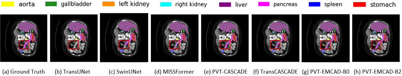
This subsection describes the qualitative results of different methods including our EMCAD. From, the qualitative results on Synapse Multi-organ dataset in Figure 4, we can see that most of the methods face challenges segmenting the left kidney (orange) and part of the pancreas (pink). However, our PVT-EMCAD-B0 (Figure 4g) and PVT-EMCAD-B2 (Figure 4h) can segment those organs more accurately (see red rectangular box) with significantly lower computational costs. Similarly, qualitative results of polyp segmentation on a representative image from ClinicDB dataset in Figure 5 show that predicted segmentation outputs of our PVT-EMCAD-B0 (Figure 5p) and PVT-EMCAD-B2 (Figure 5q) have strong overlaps with the GroundTruth mask (Figure 5r), while existing SOTA methods exhibit false segmentation of polyp (see red rectangular box).
8 Additional Ablation Study
This section further elaborates on Section 5 by detailing five additional ablation studies related to our architectural design and experimental setup.
Architectures Depth-wise convolutions Synapse ClinicDB PVT-EMCAD-B0 Sequential 81.820.3 94.570.2 PVT-EMCAD-B0 Parallel 81.970.2 94.600.2 PVT-EMCAD-B2 Sequential 83.540.3 95.150.3 PVT-EMCAD-B2 Parallel 83.630.2 95.210.2
Architectures Module Params(K) FLOPs(M) Synapse PVT-EMCAD-B0 AG 31.62 15.91 81.74 PVT-EMCAD-B0 LGAG 5.51 5.24 81.97 PVT-EMCAD-B2 AG 124.68 61.68 83.51 PVT-EMCAD-B2 LGAG 11.01 10.47 83.63
8.1 Parallel vs. sequential depth-wise convolution
We have conducted another set of experiments to decide whether we use multi-scale depth-wise convolutions in parallel or sequential. Table 7 presents the results of these experiments which show that there is no significant impact of the arrangements though the parallel convolutions provide a slightly improved performance (0.03% to 0.15%). We also observe higher standard deviations among runs in the case of sequential convolutions. Hence, in all our experiments, we use multi-scale depth-wise convolutions in parallel.
Architectures Pretrain Average Aorta GB KL KR Liver PC SP SM DICE HD95 mIoU PVT-EMCAD-B0 No 77.47 19.93 66.72 81.96 69.41 83.88 74.82 93.45 54.41 88.97 72.85 PVT-EMCAD-B0 Yes 81.97 17.39 72.64 87.21 66.62 87.48 83.96 94.57 62.00 92.66 81.22 PVT-EMCAD-B2 No 80.18 18.83 70.21 85.98 68.10 84.62 79.93 93.96 61.61 90.99 76.23 PVT-EMCAD-B2 Yes 83.63 15.68 74.65 88.14 68.87 88.08 84.10 95.26 68.51 92.17 83.92
DS EM BUSI Clinic Kvasir ISIC18 Synapse ACDC No 95.74 79.64 94.96 92.51 90.74 82.03 92.08 Yes 95.53 80.25 95.21 92.75 90.96 83.63 92.12
Architectures Resolutions FLOPs(G) DICE PVT-EMCAD-B0 0.64 81.97 PVT-EMCAD-B0 0.84 82.63 PVT-EMCAD-B0 1.89 84.81 PVT-EMCAD-B0 3.36 85.52 PVT-EMCAD-B2 4.29 83.63 PVT-EMCAD-B2 5.60 84.47 PVT-EMCAD-B2 12.59 85.78 PVT-EMCAD-B2 22.39 86.53
8.2 Effectiveness of our large-kernel grouped attention gate (LGAG) over attention gate (AG)
Table 8 presents experimental results of EMCAD with original AG [41] and our LGAG. We can conclude that our LGAG achieves better DICE scores with significant reductions in #Params (82.57% for PVT-EMCAD-B0 and 91.17% for PVT-EMCAD-B2) and #FLOPs (67.06% for PVT-EMCAD-B0 and 83.03% for PVT-EMCAD-B2) than AG. The reduction in #Params and #FLOPs is bigger for the larger models. Therefore, our LGAG demonstrates improved scalability with models that have a greater number of channels, yielding enhanced DICE scores.
8.3 Effect of transfer learning from ImageNet pre-trained weights
We conduct experiments on the Synapse multi-organ dataset to show the effect of transfer learning from the ImageNet pre-trained encoder. Table 9 reports the results of these experiments which show that transfer learning from ImageNet pre-trained PVT-v2 encoders significantly boosts the performance. Specifically, for PVT-EMCAD-B0, the DICE, mIoU, and HD95 scores are improved by 4.5%, 5.92%, and 2.54, respectively. Likewise, for PVT-EMCAD-B2, the DICE, mIoU, and HD95 scores are improved by 3.45%, 4.44%, and 3.15, respectively. We can also conclude that transfer learning has a comparatively greater impact on the smaller PVT-EMCAD-B0 model than the larger PVT-EMCAD-B2 model. For individual organs, transfer learning significantly boosts the performance of all organ segmentation, except the Gallbladder (GB).
8.4 Effect of deep supervision
We have conducted an ablation study that drops the Deep Supervision (DS). Results of our PVT-EMCAD-B2 on seven datasets are given in Table 10. Our PVT-EMCAD-B2 with DS achieves slightly better DICE scores in six out of seven datasets. Among all the datasets, the DS has the largest impact on the Synapse Multi-organ dataset.
8.5 Effect of input resolutions
Table 11 presents the results of our PVT-EMCAD-B0 and PVT-EMCAD-B2 architectures with different input resolutions. From this table, it is evident that the DICE scores improve with the increase in input resolution. However, these improvements in DICE score come with the increment in #FLOPs. Our PVT-EMCAD-B0 achieves an 85.52% DICE score with only 3.36G FLOPs when using inputs. On the other hand, our PVT-EMCAD-B2 achieves the best DICE score (86.53%) with 22.39G FLOPs when using inputs. We also observe that our PVT-EMCAD-B2 with 5.60G FLOPs when using inputs shows a 1.05% lower DICE score than PVT-EMCAD-B0 with 3.36G FLOPs. Therefore, we can conclude that PVT-EMCAD-B0 is more suitable for larger input resolutions than PVT-EMCAD-B2.