Embedding classical dynamics in a quantum computer
Abstract
We develop a framework for simulating measure-preserving, ergodic dynamical systems on a quantum computer. Our approach provides a new operator-theoretic representation of classical dynamics by combining ergodic theory with quantum information science. The resulting quantum embedding of classical dynamics (QECD) enables efficient simulation of spaces of classical observables with exponentially large dimension using a quadratic number of quantum gates. The QECD framework is based on a quantum feature map that we introduce for representing classical states by density operators on a reproducing kernel Hilbert space, . Furthermore, an embedding of classical observables into self-adjoint operators on is established, such that quantum mechanical expectation values are consistent with pointwise function evaluation. In this scheme, quantum states and observables evolve unitarily under the lifted action of Koopman evolution operators of the classical system. Moreover, by virtue of the reproducing property of , the quantum system is pointwise-consistent with the underlying classical dynamics. To achieve an exponential quantum computational advantage, we project the state of the quantum system onto a finite-rank density operator on a -dimensional tensor product Hilbert space associated with qubits. By employing discrete Fourier-Walsh transforms of spectral functions, the evolution operator of the finite-dimensional quantum system is factorized into tensor product form, enabling implementation through an -channel quantum circuit of size and no interchannel communication. Furthermore, the circuit features a state preparation stage, also of size , and a quantum Fourier transform stage of size , which makes predictions of observables possible by measurement in the standard computational basis. We prove theoretical convergence results for these predictions in the large-qubit limit, . In light of these properties, QECD provides a consistent, exponentially scalable, stochastic simulator of the evolution of classical observables, realized through projective quantum measurement. We demonstrate the consistency of the scheme in prototypical dynamical systems involving periodic and quasiperiodic oscillators on tori. These examples include simulated quantum circuit experiments in Qiskit Aer, as well as actual experiments on the IBM Quantum System One.
I Introduction
Ever since a seminal paper of Feynman in 1982 [1], the problem of identifying physical systems that can faithfully and efficiently simulate large classes of other systems (performing, in Feynman’s words, universal computation) has received considerable attention. Under the operating principle that nature is fundamentally quantum mechanical, and with the realization that simulating quantum systems by classical systems is exponentially hard, much effort has been focused on the design of universal simulators of quantum systems. Such efforts are based on the axioms of quantum mechanics, with gates connected in quantum circuits performing unitary (and thus reversible) transformations of quantum states [2, 3, 4, 5, 6, 7].
Over the past decades, several numerically hard problems have been identified, for which quantum algorithms are significantly faster than their classical counterparts. A prominent example is the Grover search algorithm, which results in a quadratic speedup over classical search [8]. In a few cases, such as random sampling, quantum computers have solved problems that would be effectively unsolvable with present-day classical supercomputing resources, thus opening the way to quantum supremacy [9]. See also Ref. [10] for a discussion of the result in Ref. [9].
Yet, at least at the level of effective theories, a great variety of phenomena are well described by classical dynamical systems, generally formulated as systems of ordinary or partial differential equations. Since simulating a quantum system by a classical system can be exponentially hard, it is natural to ask whether simulation of a classical system by a quantum system is an exponentially “easy” problem, enabling a substantial increase in the complexity and range of computationally amenable classical phenomena.
The possibility to simulate classical dynamical systems on a quantum computer has attracted growing attention, on par with research on fundamental new quantum algorithms and their practical implementation [11]. Already 20 years ago, for example, Benenti et al. [12] studied the sawtooth map generating rich and complex dynamics. The implementation of an Euler method to solve systems of coupled nonlinear ordinary differential equations (ODEs) was addressed by Leyton and Osborne [13]. A framework for sequential data assimilation (filtering) of partially observed classical systems based on the Dirac–von Neumann formalism of quantum dynamics and measurement was proposed in Ref. [14]. The simulation of classical Hamiltonian systems using a Koopman–von Neumann approach was studied by Joseph [15]. This quantum computational framework was shown to be exponentially faster than a classical simulation when the Hamiltonian is represented by a sparse matrix. More recently, the potential of quantum computing for fluid dynamics, in particular turbulence, was explored in Refs. [16, 17]. This includes, for example, transport simulators for fluid flows in which the formal analogy between the lattice Boltzmann method and Dirac equation is used [18]. Lubasch et al. [19] took a different path inspired by the success of quantum computing in solving optimization problems, modeling the one-dimensional Burgers equation by a variational quantum computing method, made possible by its correspondence with the nonlinear Schrödinger equation. Quantum systems have also been employed in the modeling of classical stochastic processes, where they have shown a superior memory compression [20, 21].
Here, we present a procedure for simulating a classical, measure-preserving, ergodic dynamical system by means of a finite-dimensional quantum mechanical system amenable to quantum computation. Combining operator-theoretic techniques for classical dynamical systems with the theory of quantum dynamics and measurement, our framework leads to exponentially scalable quantum algorithms, enabling the simulation of classical systems with otherwise intractably high-dimensional spaces of observables. Our work thus opens a novel route to the full realization of quantum advantage in the computation of classical dynamical systems.
Another noteworthy aspect of our approach is that it interfaces between classical [22, 23, 24, 25, 26, 27, 28, 29] and quantum [30, 31, 32, 33, 34, 35, 36] machine learning techniques based on kernel methods. Connections with other data-driven, operator-theoretic techniques for classical dynamics [37, 38, 39, 40, 41, 42, 43] are also prevalent. Building on our previous work on quantum mechanical approaches data assimilation [14], the framework presented here offers a mathematically rigorous route to representing complex, high-dimensional classical dynamics on a quantum computer. The primary contributions of this work are as follows.

-
wide
We present a generic pipeline that casts classical dynamical systems in terms amenable to quantum computation. This approach consists of four steps. (a) A dynamically consistent embedding of the classical state space into the state space of an infinite-dimensional quantum system with a diagonalizable Hamiltonian. (b) Eigenspace projection of the infinite-dimensional quantum system onto a finite-dimensional system, whose dynamics are representable by composition of basic commuting unitary transformations, realizable via quantum gates. (c) A preparation process, encoding the classical initial state in to a quantum computational state. (d) A quantum measurement process in the standard basis of the quantum computer to yield predictions for observables. These four steps result in simulations of a -dimensional space of classical observables using qubits and a circuit of size (i.e., number of quantum gates) and depth . We call this framework for encoding a classical dynamical system in terms of a quantum computational system quantum embedding of classical dynamics (QECD).
-
wiide
We develop the principal mathematical tools employed in this construction using Koopman and transfer operator techniques [44, 45] and the theory of reproducing kernel Hilbert spaces (RKHSs) [46, 47] and Banach function algebras on locally compact abelian groups [48, 49, 50]. The connection between the dynamical system and the Koopman operator is illustrated in Fig. 1. Using RKHSs as the foundation to build quantum mechanical models (as opposed to the spaces employed in Ref. [25]) leads to pointwise consistency with the underlying classical dynamical system; that is, consistency for every classical initial condition, rather than in the sense of expectations over initial conditions. This result should be of independent interest in the broader context of representations of classical dynamics in terms of quantum systems, which has received significant attention [51, 52, 53, 54, 55].
-
wiiide
In the particular setting of quantum computation, we establish theoretical convergence results for the finite-dimensional systems generated by the compiler, including asymptotic convergence rates in the large-qubit limit, . The time evolution of the quantum computational systems leverages discrete Fourier-Walsh techniques [56] to efficiently represent the Koopman operator using a circuit of size and depth . The state preparation step, which is a major challenge in quantum computing [57, 58], is also carried with a circuit of size and depth . In particular, we take advantage of the fact that every quantum state associated with a classical initial state in can be reached to any desired accuracy by efficient unitary transformations applied to a uniform-superposition state constructed using Hadamard gates. Meanwhile, the measurement process employs the quantum Fourier transform (QFT) to perform efficient approximate diagonalization of observables with a circuit of size and depth [59, 60].
-
wivde
We demonstrate the QECD framework in simple, analytically solvable examples of classical dynamics, so that all steps of the procedure are fully reproducible. Specifically, we use QECD to simulate the evolution of observables of periodic and quasiperiodic dynamical systems in a one- and two-dimensional phase space, respectively. We employ the gate-based, universal quantum computing toolkit Qiskit Aer [61, 62], using up to qubits. Results from simulated quantum circuit experiments (see Figs. 6 and 8) are found to be in good agreement with the true classical dynamics. In addition, we perform experiments for the periodic system on an actual quantum computer, the IBM Quantum System One, demonstrating the ability of QECD to simulate a classical system on a noisy intermediate-scale quantum (NISQ) device.
We note that the two-dimensional quasiperiodic dynamics in our examples can be straightforwardly extended to higher dimensions, where the dynamics becomes increasingly indistinguishable from a chaotic system. For quasiperiodic dynamics, no interchannel communication is necessary. Circuits of higher complexity that create inter-qubit entanglement may need to be explored for treatment of chaotic dynamics.
The outline of the paper is as follows. First, in Sec. II we give a high-level description of the methodological framework underlying the quantum embedding. In Sec. III, we introduce the class of dynamical systems under study, along with the corresponding RKHSs of classical observables. This is followed in Secs. IV–VIII by a detailed description of the construction of the QECD for this class of systems. In Secs. IX and X, we present our results from simulated and actual quantum computation experiments, respectively. Our primary conclusions are summarized in Sec. XI. The paper contains appendices on RKHS-based quantum mechanical representations of classical systems (Appendix A), Fourier-Walsh factorization of the Koopman generator (Appendix B), and QFT-based approximate diagonalization of observables (Appendix C). In addition, we provide an overview of elements of Koopman operator theory related to this work and associated numerical techniques as supplementary material (SM) [63].
II A route to quantum embedding of classical dynamics
We begin by describing the main components of the QECD framework for representing classical dynamics on a quantum computer. Figure 2 schematically summarizes the successive levels used in the procedure, passing through classical, classical statistical, infinite-dimensional quantum mechanical, finite-dimensional quantum mechanical (referred to as matrix mechanical), and quantum computational levels. This diagram juxtaposes the steps for states and observables side-by-side for easy comparison. In the following subsections, we discuss the individual horizontal and vertical connections (which are maps) on each of the five levels of this diagram.

II.1 Classical and classical statistical levels
Consider a classical dynamical system on a compact metric space , described by a dynamical flow map
| (1) |
as indicated by a horizontal arrow in the left-hand column of Fig. 2. The classical state space is embedded into the space of Borel probability measures (i.e., the classical statistical space) by means of the map sending to the Dirac measure supported at . The dynamics acts naturally on the classical statistical space by the pushforward map on measures,
| (2) |
also known as the transfer or Perron-Frobenius operator [44, 45]. The map has the equivariance property , represented by the top loop in the the left-hand column in Fig. 2.
Associated with the dynamical system are spaces of classical observables, which we take here to be spaces of complex-valued functions on . A natural example is the space of continuous functions, denoted as , which also forms an (abelian) algebra with respect to the pointwise product of functions. The Koopman operator [64, 65], , acts on observables in by composition with the flow map, i.e.,
| (3) |
see also Fig. 1. The horizontal arrow in the first line of the right-hand column in Fig. 2 represents the action of the Koopman operator on a subalgebra that will be described in Sec. II.2 below.
In this context, a simulator of the system can be described as a procedure which takes as an input an observable and an initial condition , and produces as an output a function approximating the evolution of the observable under the dynamics. For instance, if is the flow generated by a system of ODEs on , and is an invariant subset of this flow (e.g., an attractor), a standard simulation approach is to construct a finite-difference approximation of the dynamical flow based on a timestep (using interpolation to generate a continuous-time trajectory), and obtain by evaluating the observable of interest on the approximate trajectory. The scheme then converges in a limit of by standard results in ODE theory and numerical analysis for observables of sufficient regularity.
From an observable-centric standpoint, a simulator of the system corresponds to a linear operator approximating the Koopman operator , giving . For instance, the ODE-based approximation just mentioned can be described in this way for , but note that not every approximation of has to be of the form of a composition operator by a flow. Indeed, “lifting” the task of simulation from states to (classical) observables opens the possibility of using new approximation techniques, which in some cases can resolve computational bottlenecks, e.g., due to high dimensionality () of the ambient state space [66]. Invariably, every practical simulator is restricted to act on a space of observables of finite dimension, (e.g., a subspace of or ). In general, the computation cost of acting with on elements of this space scales as , but can be reduced to if is efficiently represented by a diagonal matrix. The evaluation cost of observables, which corresponds to summation of an -term basis expansion such as a Fourier series, is typically .
In what follows, rather than employing an approximation acting on classical observables, our goal is to simulate the action of using a quantum mechanical system. As we will see, this can be achieved at a logarithmic cost of elementary quantum operations (gates); specifically, QECD allows simulation of spaces of classical observables of dimension using gates.
II.2 Quantum computational representation
The QECD framework effecting the representation of the classical system by a quantum mechanical system employs the following key spaces:
-
1.
The classical state space .
-
2.
A Banach ∗-algebra of classical observables.
-
3.
An infinite-dimensional RKHS .
-
4.
A finite-dimensional Hilbert space associated with the quantum computer.
The Hilbert spaces and have corresponding (non-abelian) algebras of bounded linear operators, and , respectively, acting as quantum mechanical observables. Moreover, states on these algebras are represented by density operators, i.e., trace-class, positive operators of unit trace, acting on the respective Hilbert space. We denote the spaces of density operators on and by and , respectively. Below, represents the number of qubits, thus the dimension of is .
The spaces of classical states and observables and are mapped into the spaces of quantum states and observables and , respectively; see Fig. 2. The following maps on states (left-hand column) and observables (right-hand column) transform the classical system into a quantum-mechanical one on :
-
•
We construct a map from classical states (points) in to quantum states on . By analogy with the RKHS-valued feature maps in machine learning [67], will be referred to as a quantum feature map. To arrive at , the classical statistical space is first embedded into the quantum mechanical state space associated with through a map (see (22) below). The composite map thus describes a one-to-one quantum feature map from into . Next, the infinite-dimensional space is projected onto a finite-dimensional quantum state space associated with a -dimensional subspace by means of a map . We refer to this level of description as matrix mechanical since all quantum states and observables are finite-rank operators, represented by matrices. To arrive at the quantum computational state space, we finally apply a unitary , so that the full quantum feature map from to takes the form .
-
•
We construct a linear map from classical observables in to quantum mechanical observables in . This map takes the form , where is a projection, so that yields a quantum computational representation of classical observables passing through intermediate quantum mechanical and matrix mechanical representations. Here, is one-to-one on real-valued functions in , and is self-adjoint whenever is real.
Next, we describe the maps governing the temporal evolution of states and observables, represented by horizontal arrows in Fig. 2:
-
•
At the quantum mechanical level, states in evolve under the operator (horizontal arrow in the left-hand column) induced by a unitary Koopman operator on . This evolution is generated by a skew-adjoint generator , defined on a dense subspace and possessing a countable spectrum of eigenfrequencies.
-
•
The generator is mapped to a self-adjoint Hamiltonian given by . This Hamiltonian is decomposable as a sum of mutually-commuting operators , each of which is of pure tensor product form, . The latter property enables quantum parallelism in the unitary evolution at the quantum computational level generated by (see horizontal arrow at the bottom of the left-hand column of Fig. 2). One of our main results is that can be implemented via a quantum circuit of size and no interchannel communication (see Figs. 6 and 8).
-
•
The horizontal arrow at the quantum mechanical level represents the action of the Heisenberg evolution operator . Under the assumption that the RKHS is invariant under the Koopman operator, acts on by conjugation with , i.e., .
-
•
The corresponding Heisenberg evolution operator at the quantum computational level, , acting on quantum mechanical observables on the Hilbert space , is represented by the horizontal arrow at the bottom of the right-hand column. This operator is obtained by projection of , viz. .
Given a classical initial condition , the quantum computational system constructed by QECD makes probabilistic predictions of through quantum mechanical measurement of the projection-valued measure (PVM) [4, 68] associated with the quantum register on the quantum state , where . The state is prepared by means of a circuit of size , which is applied to the standard initial state vector of the quantum computer. Furthermore, the measurement step is effected by performing a rotation by a QFT, which is implementable via a circuit of size . An ensemble of such measurements then approximates the quantum mechanical expectation value
| (4) |
The function converges in turn uniformly to the true classical evolution, i.e., , in the large-qubit limit, . We will return to these points in a more detailed discussion in Secs. V–VIII.
In summary, the key distinguishing aspects of QECD are as follows:
-
wide
Dynamical consistency. The predictions made by the quantum quantum computational system via (4) converge to the true classical evolution as the number of qubits increases. In particular, since , the convergence is exponentially fast in .
-
wiide
Quantum efficiency. The full circuit implementation of the scheme, including state preparation, dynamical evolution, and measurement, requires a circuit of size and depth . Since, as just mentioned, the dimension of increases exponentially with , the quantum computational system constructed by QECD has an exponential advantage over classical simulators of the underlying -dimensional subspace of classical observables.
-
wiiide
State preparation. The quantum computational state corresponding to classical state is prepared by passing the standard initial state vector of the quantum computer through a circuit of size and depth . This overcomes the expensive (potentially exponential) state preparation problem affecting many quantum computational algorithms.
-
wivde
Measurement process. The process of querying the system to obtain predictions is a standard projective measurement of the quantum register. Importantly, no quantum state tomography or auxiliary classical computation is needed to retrieve the relevant information.
III Classical dynamics and observables
III.1 Dynamical system
We focus on the class of continuous, measure-preserving, ergodic flows with a pure point spectrum generated by finitely many eigenfrequencies and continuous corresponding eigenfunctions. Every such system is topologically conjugate (for our purposes, equivalent) to an ergodic rotation on a -dimensional torus, so we will set without loss of generality. Using the notation to represent a point , where are canonical angle coordinates, the dynamics is described by the flow map
| (5) |
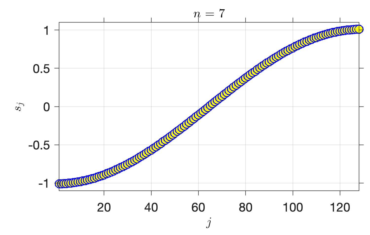
where are positive, rationally independent (incommensurate) frequency parameters. This dynamical system is also known as a linear flow on the -torus, but note that is not a linear space. In dimension , the orbits of the dynamics do not close by incommensurability of the , each forming a dense subset of the torus (i.e., a given orbit passes by any point in at an arbitrarily small distance). The case is shown for two choices of in Fig. 3, illustrating the difference between ergodic and non-ergodic dynamics. In dimension , the flow map corresponds to a harmonic oscillator on the circle, , where each orbit is periodic and samples the whole space.
It is important to note that if the dynamical system is not presented in the form of a torus rotation, then standard constructions from ergodic theory may be used to transform it into the form in (5). These constructions are based entirely on spectral objects (i.e., eigenfunctions and eigenfrequencies) associated with the Koopman operator of the system. See Sec. I D in the SM for further details [63]. The same constructions allow one to treat the case where is a periodic or quasiperiodic attractor of a dynamical flow on a higher-dimensional space . By virtue of these facts, the quantum mechanical framework described in this paper can readily handle simulations of observables of general measure-preserving, ergodic flows with pure point spectrum. Relevant examples include ODE models on with quasiperiodic attractors [69], as well as PDE models where is an infinite-dimensional function space. The latter class includes many pattern-forming physical systems such as thermal convection flows [70], plasmas [71], and reaction-diffusion systems [72] in moderate-forcing regimes.

At any dimension , the flow in (5) is measure-preserving and ergodic for a probability measure given by the normalized Haar measure. The dynamics of classical observables is governed by the Koopman operator , which is a linear operator, acting by composition with the dynamical flow in accordance with (3) [44, 73, 45]. The Koopman operator acts as an isometry on the Banach space of continuous functions on , i.e., , where is the uniform norm. In addition, lifts to a unitary operator on the Hilbert space associated with the invariant measure. That is, using to denote the inner product, we have for all , which implies, in conjunction with the invertibility of , that
Here, denotes the operator adjoint, which is also frequently denoted as . The collection then forms a strongly continuous unitary group under composition of operators 111This implies (i) , (ii) , and (iii) for all and .. See again Fig. 1.
By Stone’s theorem on one-parameter unitary evolution groups [75], the Koopman group on has a skew-adjoint infinitesimal generator, i.e., an operator defined on a dense subspace satisfying
| (6) |
for all . The generator gives the Koopman operator at any time by exponentiation,
| (7) |
Modulo multiplication by to render it self-adjoint, it plays an analogous role to a quantum mechanical Hamiltonian generating the unitary Heisenberg evolution operators.
As already noted, the torus rotation in (5) is a canonical representative of a class of continuous-time continuous dynamical systems on topological spaces with quasiperiodic dynamics generated by finitely many basic frequencies. This means that every such system can be transformed into an ergodic torus rotation of a suitable dimension by a homeomorphism (continuous, invertible map with continuous inverse). By specializing to this class of systems (as opposed to a more general measure-preserving, ergodic flow), we gain two important properties:
-
wide
The dynamics has no mixing (chaotic) component. This implies that the spectrum of the Koopman operator for this system acting on , or a suitable RKHS as in what follows, is of “pure point” type, obviating complications arising from the presence of continuous spectrum as would be the case under mixing dynamics.
-
wiide
The state space is a smooth, closed manifold with the structure of a connected, abelian Lie group. The abelian group structure, in particular, renders this system amenable to analysis with Fourier analytic tools.
Below, we use a -dimensional vector to represent a generic multi-index, and
| (8) |
to represent the Fourier functions on . In Sec. XI, we will discuss possible avenues for extending the framework presented here to other classes of dynamical systems, such as mixing dynamical systems with continuous spectra of the Koopman operators.
III.2 Algebra of observables
According to the scheme described in Sec. II.2, we perform quantum conversion of an (abelian) algebra of classical observables, i.e., a space of complex-valued functions on which is closed under the pointwise product of functions. We construct such that it is a subalgebra of with additional (here, ) regularity and RKHS structure. This structure is induced by a smooth, positive-definite kernel function , which has the following properties for every point and function :
-
1.
The kernel section lies in .
-
2.
Pointwise evaluation, , is continuous, and satisfies
(9) where is the inner product of .
Equation (9) is known as the reproducing property, and underlies the many useful properties of RKHSs for tasks such as function approximation and learning. Note, in particular, that spaces, which are more commonly employed in Koopman operator theory and numerical techniques (see Sec. III.1), do not have a property analogous to (9). In fact, pointwise evaluation is not even defined for the Hilbert space on . See Refs. [76, 46, 47] for detailed expositions on RKHS theory.
Our construction of follows Ref. [50]. We begin by setting parameters and , and defining the map ,
and the functions ,
We then define a kernel via the series
| (10) |
where the sum over converges uniformly on to a smooth function. Intuitively, can be thought of as a locality parameter for the kernel, meaning that as decreases becomes increasingly concentrated near , approaching a -function as .
An important property of the kernel that holds for any is that it is translation-invariant on the abelian group . That is, using additive notation to represent the binary group operation on , we have
| (11) |
In particular, setting , where is the identity element of , and noticing that the dynamical flow from (5) satisfies , we deduce the dynamical invariance property
In Ref. [50] it was shown that for every and , the kernel in (10) is a strictly positive-definite kernel on , so it induces an RKHS, , which is a dense subspace of . One can verify that the collection forms an orthonormal basis of , consisting of scaled Fourier functions, so every observable admits the expansion
where the sum over converges in norm. The above manifests the fact that contains continuous functions with Fourier coefficients decaying faster than any polynomial, implying in turn that every element of is a smooth function in .
It can also be shown that the RKHS induced by acquires an important special property which is not shared by generic RKHSs—namely, it becomes an abelian, unital, Banach ∗-algebra under pointwise multiplication of functions. We list the defining properties for completeness in Appendix A.1. In Ref. [50], the space was referred to as a reproducing kernel Hilbert algebra (RKHA) as it enjoys the properties of both RKHSs and Banach algebras. In particular, a distinguishing aspect of is that it simultaneously has Hilbert space structure (as ) and Banach ∗-algebra structure (as ), while also allowing pointwise evaluation by continuous functionals, (i.e., the reproducing property in (9)). The RKHAs associated with the family of kernels in (10) are examples of harmonic Hilbert spaces on locally compact abelian groups [48], and are also closely related (by Fourier transforms) to weighted convolution algebras [49] on the dual group of .
Table 1 summarizes the properties of and other function spaces on employed in this work. In what follows, we shall let denote the set of self-adjoint elements of , i.e., the elements satisfying . Since the ∗ operation of corresponds to complex conjugation of functions, it follows that contains the real-valued functions in . Note that if is an element of , then its expansion coefficients in the basis satisfy .
Next, we state a product formula for the orthonormal basis functions , which follows directly from their definition, viz.
| (12) |
In the above, we interpret the coefficients as “structure constants” of the RKHA . Figure 4 displays representative matrices formed by the in dimension and 2 for and .


In the special case , we will let be the RKHA on the circle constructed as above. We denote the reproducing kernel of by , and let , , be the corresponding orthonormal basis functions with . It then follows that admits the tensor product factorization
| (13) |
and the reproducing kernel and orthonormal basis functions of similarly factorize as
where , and , are canonical angle coordinates of the points , , respectively (see also (8)).
| Completeness | ✓ | ✓ | ✓ | ✓ | |
| Hilbert space structure | ✓ | ✓ | |||
| Pointwise evaluation | ✓ | ✓ | ✓ | ||
| ∗-algebra structure | ✓ | ✓ | ✓ | ✓ | |
| regularity | ✓ | ✓ |
III.3 Evolution of RKHA observables
From an operator-theoretic perspective, simulating the dynamical evolution of a continuous classical observable can be understood as approximating the Koopman operator on ; for, if were known one could use it to compute for every observable , time , and initial condition (cf. Sec. II). Yet, despite its theoretical appeal, consistently approximating the Koopman operator on is challenging in practice, as this space lacks the Hilbert space structure underpinning commonly employed operations used in numerical techniques, such as orthogonal projections (see Table 1). For a measure-preserving, ergodic dynamical system such as the torus rotation in (5), a natural alternative is to consider the unitary Koopman operator on the Hilbert space associated with the invariant measure . While this choice addresses the absence of orthogonal projections on , lacks the notion of pointwise evaluation of functions, so one must correspondingly abandon the notion of pointwise forecasting in this space.
In light of the above considerations, RKHSs emerge as attractive candidates of spaces of classical observables in which to perform simulation, as they allow pointwise evaluation through the reproducing property in (9) while having a Hilbert space structure. Unfortunately, an obstruction to using RKHSs in dynamical systems forecasting is that a general RKHS on need not be preserved under the dynamics, even if the reproducing kernel is continuous. That is, in general, if lies in an RKHS, the composition need not lie in the same space, and thus the Koopman operator is not well-defined as an operator mapping the RKHS into itself [27]. Intuitively, this is because membership of a function in an RKHS generally imposes stringent requirements in its regularity, as we discussed for example in Sec. IV.1 with the rapid decay of Fourier coefficients, which need not be preserved by the dynamical flow.
An exception to this obstruction occurs when the reproducing kernel is translation-invariant, which holds true for the class of kernels introduced in Sec. III.2 (see (11)). In fact, it can be shown [55] that the RKHA associated with the kernel in (10),is invariant under the Koopman operator for all , and is unitary and strongly continuous. Analogously to the case, the evolution group is uniquely characterized through its skew-adjoint generator , defined on a dense subspace , and acting on observables as displayed in (6).
For the torus rotation in (5), is diagonalizable in the basis of . That is, for , we have
where is a real eigenfrequency given by
| (14) |
Moreover, admits a decomposition into mutually commuting, skew-adjoint generators satisfying
| (15) |
In particular, since is an orthonormal basis, (15) completely characterizes , and we have
| (16) |
It should be noted that the Koopman generator on admits a similar decomposition to (16); see e.g., Ref. [25] for further details. Analogously to the case, the Koopman operator on can be recovered at any from the generator by exponentiation as given in (7).
IV Embedding into an infinite-dimensional quantum system
The initial stages of the QECD procedure outlined in Sec. II involve embedding classical states and observables into states and observables of quantum system associated with an infinite-dimensional RKHS , arriving at the quantum mechanical level depicted in Fig. 2. In this section, we describe the construction of this quantum system and associated embeddings of classical states and observables. First, in Sec. IV.1 we build as a subspace of the RKHA from Sec. III.2. Then, in Secs. IV.2 and IV.3 we establish representation maps and from classical states and observables into quantum mechanical states and observables, respectively, on . Note that the quantum mechanical embedding of states passes through an intermediate classical statistical level associated with probability measures on the classical state space (second row in the left-hand column of Fig. 2). In Secs. IV.4 and IV.5, we establish the classical-quantum consistency and associated dynamical properties of our embeddings.
IV.1 Reproducing kernel Hilbert space
We choose as an infinite-dimensional subspace of the RKHA containing zero-mean functions. For that, we introduce the (infinite) index set
| (17) |
and define as the corresponding infinite-dimensional closed subspace
The space is then an RKHS with the reproducing kernel
| (18) |
In particular, for every , which is necessarily an element of , the reproducing property in (9) reads
where is the section of the kernel at , and denotes the inner product of .
By excluding zero indices from the index set , every element of has zero mean, , as noted above. The reason for adopting this particular definition for , instead of, e.g., working with the entire space , is that later on it will facilitate construction of -dimensional subspaces suitable for quantum computation (see Sec. V). In what follows, will denote the orthogonal projection with . Moreover, we set
where these definitions are independent of the point by (11). We also note that, by construction, is a Koopman-invariant subspace of , so we may define unitary Koopman operators by restriction of from Sec. III.3.
IV.2 Representation of states with a quantum feature map
For our purposes, a key property that the RKHS structure of endows is the feature map, which is the continuous map mapping classical state to the RKHS function
| (19) |
It can be shown that for the choice of kernel in (18), is an injective map, and the functions are linearly independent. It is then natural to think of the normalized feature vectors
| (20) |
as “wavefunctions” corresponding to classical states .
We can generalize this idea by associating every such wavefunction with the pure quantum state . The mapping with
| (21) |
then describes an embedding of the classical state space into quantum mechanical states in , which we refer to as a quantum feature map. Note that there is no loss of information in representing by . Moreover, can be understood as a composition , where maps classical state to the Dirac probability measure , and is a map from classical probability measures on to quantum states on , such that
| (22) |
The map describes an embedding of the state space into the space of probability measures , i.e., the classical statistical level in the left-hand column of Fig. 2. See Ref. [50] for further details on the properties of this map.
By virtue of it being an RKHS, we can also define classical and quantum feature maps for the RKHA . Specifically, we set and , where
| (23) |
and . The feature maps and have analogous properties to and , respectively, which we do not discuss here in the interest of brevity.
IV.3 Representation of observables
The quantum mechanical representation of classical observables in is considerably facilitated by the Banach algebra structure of that space. In Sec. IV.3.1, we leverage that structure to build representation maps from functions in to bounded linear operators in . Then, in Sec. IV.3.2, we consider associated representations mapping into bounded linear operators on the RKHS (which is a strict subspace of ), arriving at the map depicted in the right-hand column of Fig. 2. Additional details on the construction are provided in Appendix A.
IV.3.1 Representation on the RKHA
We begin by noting that the joint continuity of the multiplication operation of Banach algebras (see (81)) implies that for every the multiplication operator is well-defined as a bounded operator in . This leads to the regular representation , which is the algebra homomorphism of into , mapping classical observables in to their corresponding multiplication operator,
| (24) |
This mapping is a homomorphism since
and it is injective (i.e., faithful as a representation) since whenever . However, is not a ∗-representation; i.e., is not necessarily equal to . In particular, need not be a self-adjoint operator in if is a self-adjoint element in . To construct a map from into the self-adjoint operators in , we define with
| (25) |
By construction, is self-adjoint for all , and it can also be shown (see Appendix A.2) that is injective on . That is, provides a one-to-one mapping between real-valued functions in and self-adjoint operators in .


It follows from the product formula in (III.2) that if has the expansion , where , then the corresponding multiplication operator has the matrix elements
and thus
| (26) |
Correspondingly, the matrix elements of the self-adjoint operator are given by
If, in addition, lies in , then we have and the formula above reduces to
| (27) |
Here, of particular interest are the multiplication and self-adjoint operators representing the basis elements of , i.e., and , respectively, for . Since for , it follows from (26) that after a suitable lexicographical ordering of multi-indices (as in Fig. 4), forms a banded matrix with nonzero elements only in the diagonal corresponding to multi-index . Figure 5(a) illustrates the nonzero matrix elements of in the one-dimensional case, . Similarly, the self-adjoint operator is a bi-diagonal matrix with nonzero entries in the diagonals corresponding to , as shown in Fig. 5(b).
We deduce from these observations that if is a bandlimited observable (i.e., expressible as a finite linear combination of Fourier functions ), is represented by a banded matrix, whose -th diagonal comprises of the structure constants multiplied by . The matrix representing is also banded whenever is bandlimited. If, in addition, is real, the -th diagonal of is given by the multiple of with .
IV.3.2 Representation on the RKHS
We now take up the task of defining analogs of the maps and from Sec. IV.3.2, mapping elements of to bounded operators on the RKHS (i.e., the Hilbert space underlying the infinite-dimensional system at the quantum mechanical level). To that end, let be the projection map from to , defined as
| (28) |
where is the orthogonal projection from to introduced in Sec. IV.1. One can explicitly verify that the map is injective, so there is no loss of information in representing by as opposed to . For our purposes, however, in addition to injectivity we require that our representation maps provide value-level consistency between classical and quantum measurements (in a sense made precise in Sec. IV.4 below). For that, it becomes necessary to modify the map , as well as its self-adjoint counterpart , to take into account the contractive effect of the projection .
In Appendix A.3, we construct a self-adjoint, invertible operator , which is diagonal in the basis, and whose role is to counter-balance that contraction. Specifically, we define and with
| (29) |
Here, inflates the expansion coefficients of functions in the basis of , absorbing the contractive action of . Analogously to and , respectively, is one-to-one, and is one-to-one on the real functions in . Moreover, every operator in the range of is self-adjoint. The map provides the representation of classical observables in by self-adjoint operators in at the quantum mechanical level, depicted by vertical arrows in the right-hand column of Fig. 2.
IV.4 Classical–quantum consistency
We now come to a key property of the regular representation and the associated map , which is a consequence of the reproducing property and Banach algebra structure of . Namely, and provide a consistent correspondence between evaluation of classical observables and quantum mechanical expectation values. To see this, for any quantum state and quantum mechanical observable , let
| (30) |
be the standard quantum mechanical expectation functional. Then, it follows from the reproducing property in (9), the definition of the quantum feature map in (23), and the definition of the regular representation in (24) that for any observable and classical state ,
| (31) |
where . The last equality in (31) requires that is a self-adjoint element in ; see Ref. [50] for further details. Equation (31) shows, in particular, that by passing to the quantum mechanical representation we maintain pointwise consistency with the classical measurement processes for special sets of quantum mechanical observables and states. These are the self-adjoint operators and the pure states .
To express these relationships in terms of matrix elements, note first that the quantum state satisfies
| (32) |
Combining this result with (26), we obtain
and this relationship holds irrespective of whether is self-adjoint or not. If is a self-adjoint element in , then we can use the matrix elements of the self-adjoint operator from (27), in conjunction with the fact that is also self-adjoint, to arrive at the expression
Even though is a strict subspace of the RKHA , it is still possible to consistently recover all predictions made for classical observables, as we describe in Appendix A.3. There, we show that the modified versions and of and , respectively (defined in (29)), satisfy the analogous consistency relation to (31), i.e.,
| (33) |
where is the quantum state on obtained from the feature map in (21). As with (31), the first equality in (33) holds for any and the second holds for real-valued elements .
IV.5 Dynamical evolution
In this section, we describe the dynamics of quantum states and observables associated with the RKHA and RKHS , and establish consistency relations between the classical and quantum evolution.
First, recall that the Koopman operators act on as a unitary evolution group. As a result, there is an induced action on quantum mechanical observables in , given by
| (34) |
This action has the important property of being compatible with the action of the Koopman operator on functions in under the regular representation. Specifically, for every and , we have
| (35) |
The unitary evolution in (34) has a corresponding dual action on quantum states, given by
| (36) |
One can verify that this action is compatible with the classical dynamical flow under the feature map , viz.
| (37) |
Using (31), (34), and (36), we arrive at the consistency relationships
| (38) |
with . This holds for every classical observable , initial condition , and evolution time . If, in addition, is a self-adjoint element in , we may compute the evolution using the self-adjoint operator , which is accessible via physical measurements. That is, for we have
| (39) |
In summary, we have constructed a dynamically consistent embedding of the torus rotation from (5) into a quantum mechanical system on the RKHA . For completeness, we note that the matrix elements of the state are given by
Using this formula together with the expressions for the matrix elements of in (27), respectively, we arrive at the expression
which holds for all self-adjoint elements .
Our discussion was thus far based on the RKHA , as opposed to the RKHS . In Appendix A.4, we establish that the dynamics of classical states and observables can be represented consistently through their representatives on using the maps and in (29). Specifically, we show that for any ,
while for any real-valued ,
where . In the above, and are evolution operators on quantum observables and states on , respectively, defined analogously to their counterparts on using the Koopman operator (see Sec. IV.1).
V Projection to finite dimensions
While being dynamically consistent with the underlying classical evolution, the quantum system constructed in Sec. IV is infinite-dimensional, and thus not directly accessible to simulation by a quantum computer. We now describe an approach for projecting the infinite-dimensional quantum system to a finite-dimensional system. In Fig. 2 we refer to this level of representation as matrix mechanical, since all linear operators involved have finite rank and are representable by matrices. Our objectives are to construct this projection such that (a) it is refinable, i.e., the original quantum system is recovered in a limit of infinite dimension (number of qubits); and (b) it facilitates the eventual passage to the quantum computational level (to be described in Sec. VI).
We begin by fixing a positive integer parameter (the number of qubits), chosen such that it is a multiple of the dimension of the classical state space , and defining the index sets
| (40) |
Note that is a subset of from (17) with elements. Next, consider the -dimensional subspace of given by
and let be the orthogonal projection mapping into . When appropriate, we will interpret as a map into its range, i.e., , without change of notation. The subspace has the structure of an RKHS of dimension , associated with the spectrally truncated reproducing kernel
Moreover, is a nested family of subspaces, increasing towards .
By virtue of being spanned by eigenfunctions of the generator , is invariant under the Koopman operator, i.e., for all . Moreover, the projection commutes with both and ,
These invariance properties allow us to define a projected generator
| (41) |
and an associated Koopman operator
such that the following diagram commutes for all :
| (42) |
Similarly, we define a finite-rank Heisenberg operator
where is the projection on defined as . This leads to an analogous commutative diagram to that in (42) viz.,
Next, we introduce a spectrally truncated feature map , defined analogously to (19) as
as well as a corresponding quantum feature map , such that is given by
| (43) |
In the sequel, we will use the states as approximations of the states . These approximations have the following properties.
-
1.
The dynamical evolution of is governed by a finite-rank operator , where
-
2.
As (i.e., in the infinite qubit limit), converges to , in the sense that for any quantum mechanical observable ,
(44) where , and the convergence is uniform with respect to .
In light of the above, we employ the following approximations to the quantum mechanical representation of the evolution of classical observables from Sec. IV.5 (see also Appendix A.4),
| (45) | ||||
By (44), for every function and evolution time , converges as to , uniformly with respect to , whereas converges to if is self-adjoint (real-valued).
VI Representation on a quantum computer
We are now ready to perform the final step in the QECD pipeline, namely passage from the matrix mechanical level to the quantum computational level associated with the -qubit Hilbert space (see bottom row in Fig. 2). We will do so by applying a unitary map, so that the systems in the matrix mechanical and quantum computational levels are isomorphic as quantum systems. However, the key aspects that the quantum computational system provides are that (a) it can be efficiently implemented as a quantum circuit with a quadratic number of gates in ; and (b) information about the evolution of classical observables can be extracted by measurement of the standard projection-valued measure associated with the computational basis. We describe the construction of the unitary map from the matrix mechanical to quantum computational levels and the properties of the resulting quantum system in Secs. VI.1 and VI.2, respectively.
VI.1 Quantum computational system on the tensor product Hilbert space
Being expressible in terms of finite-rank quantum states, observables, and evolution operators, the approximation framework described in Sec. V can be encoded in a quantum computing system operating on a finite-dimensional Hilbert space. In particular, letting denote the 2-dimensional Hilbert space associated with a single qubit, it follows immediately from the fact that is a -dimensional Hilbert space that there exists a unitary map , where
| (46) |
is the tensor product Hilbert space associated with qubits. Under such a unitary, the projected generator from (41) maps to a skew-adjoint operator , inducing a self-adjoint Hamiltonian
| (47) |
and a corresponding unitary evolution operator on . This leads to the commutative diagram
expressing the fact that elements of and evolve consistently under and , respectively. Note that we work here with the self-adjoint Hamiltonian as opposed to the skew-adjoint generator for consistency with the usual convention in quantum mechanics.
In addition, induces a unitary , with , mapping quantum mechanical observables on to quantum mechanical observables on . The restriction of on then induces a continuous, invertible map from quantum states on to quantum states on (which we continue to denote using the symbol ). Moreover, we have the evolution maps
| (48) | ||||
such that the maps for states and observables between and within the matrix mechanical and quantum computational level in Fig. 2 constitute commutative diagrams. In particular, following the vertical arrows in the left- and right-hand columns from the classical level to the quantum computational level gives the maps and , where
| (49) | ||||
The maps and provide the quantum computational representation of classical states and observables, respectively, which are two of the main ingredients of the QECD (see Sec. II). By unitary equivalence, they have analogous convergence properties in the limit as those of their matrix mechanical counterparts and described in Sec. V.We also note that the evolution operator at the quantum computational level can be equivalently obtained as a projection of the Koopman operator on , i.e.,
| (50) |
VI.2 Factorizing the Hamiltonian in tensor product form
In order for the representation of the dynamics on to exhibit robust quantum parallelism, i.e., implementation on a quantum circuit of small depth, it is highly beneficial that the Hamiltonian can be decomposed as a sum of commuting operators in pure tensor product form, i.e.,
| (51) |
where and are mutually-commuting, single-qubit Hamiltonians. With such a decomposition, the unitary operator generated by factorizes as
| (52) |
Thus, can be split into a composition of up to unitaries (depending on the number of nonzero terms in the right-hand side of (51)), which can be applied in any order by commutativity of the . Moreover, each unitary has a generator of pure tensor product form, and thus can be represented as a quantum circuit with at most quantum gates for rotations of the individual qubits.
In fact, as we will now show, using a Walsh operator representation [56], for a dynamical system with pure point spectrum the decomposition in (51) only has nonzero terms , and for each nonzero term, the tensor product factorization has all but one factors equal to the identity. As a result,
and the decomposition in (52) reduces to a tensor product of unitaries,
| (53) |
The key point about (53) is that can be implemented via a quantum circuit of qubit channels with no cross-channel communication. We will return to this point in Sec. VII.
VI.2.1 Walsh-Fourier transform and Walsh operators
Classical states and observables of the dynamical system have been transformed into pure state density operators and self-adjoint operators on the -dimensional Hilbert space which is a tensor product of the single qubit quantum state spaces as given in (46). We will employ the commonly used Dirac bra-ket notation [5] to denote vectors in . We let be the standard orthonormal basis of the single-qubit Hilbert space comprising of eigenvectors of the Pauli operator,
with
Thus, each vector can be expanded in this basis as
| (54) |
In order to arrive at the decomposition in (53), we employ the approach developed in Ref. [56], which is based on discrete Walsh-Fourier transforms, and the associated Walsh operators, as follows. First, for any non-negative integer , we let be its binary expansion; that is,
where is the smallest positive integer such that . For example, we have , , , , and . Moreover, for every real number we let be its dyadic expansion, i.e.,
Note that the most significant digit in is the last one, , whereas the most significant digit in is the first one, .
With this notation, for every we define the Walsh function as
Furthermore, for any and , we define the discrete Walsh function of order , as
It then follows that
Here, is the -digit binary expansion of obtained by padding to the right with zeros, as needed. Moreover,
is the -digit reversed binary representation of . Thus, the exponent in the expression for is given by the inner product between the -digit binary expansion of with the bit-reversed binary expansion of . For example, with and , we have , , , and .
Among the Walsh functions , those with for are called Rademacher functions, , and satisfy
| (55) |
That is, depends only on the -th bit in the dyadic expansion of . Using (55), it follows that for any integer , we have
meaning that we can express the -th bit in the dyadic decomposition of in terms of the -th Rademacher function,
| (56) |
It is known that the set forms an orthonormal basis of the Hilbert space with respect to Lebesgue measure. In the discrete case, we let be the -dimensional Hilbert space, , with respect to the normalized counting measure supported on . Then, the set of discrete Walsh functions of order , , is an orthonormal basis of . One obtains
The map is called the discrete Walsh-Fourier transform of the function .
Next, consider the tensor product basis of with , where the multi-index runs over all binary strings of length . Whenever convenient, we will employ the notation , where . That is, is an integer in the range , whose reversed binary representation is equal to ,
For example, in a system with qubits corresponds to , where the least significant bit is the one to the right. Note that is also the standard quantum computational basis for an -qubit problem in the Qiskit framework [62, 61] that we will employ in Sec. IX 222The qubit ordering in Qiskit is reverse to that in most textbooks on quantum computing..
For every , we define the associated Walsh operator as
By construction, the form a collection of mutually-commuting, self-adjoint operators, which have pure tensor product form and are diagonal in the basis of , i.e.,
where is again a quantum computational basis vector. For example, for qubits, the Walsh operator with , and the basis vector , one obtains
It follows from a counting argument that the collection forms a basis of the vector space of operators in which are diagonal in the basis. In Ref. [56], it was shown that if is such a diagonal operator,
then it admits the expansion
| (57) |
where the expansion coefficients are the complex Walsh-Fourier coefficients of the function with . That is, is equal to the eigenvalue , where is the -digit binary representation of the integer .
VI.2.2 Walsh representation of the Hamiltonian
In order to effect the decomposition in (51) for the generator-induced Hamiltonian from (47), let be the enumeration on the index set from (40) based on the standard order of integers, i.e., . For example, , gives , which is mapped to . The mapping of (for , ) is displayed in first and third columns of Table 2. We define as the unique (unitary) linear map such that for ,
| (58) | ||||
That is, maps the basis element of with multi-index to the tensor product basis element , with given by an invertible binary string encoding of . Here, is obtained as a concatenation of binary strings of length , corresponding to the dyadic decompositions of , respectively. See again Table 2, where we list the mapping for a two-dimensional torus with qubits for each torus dimension.
Since with given by (14), we have
| (59) |
Thus, in order to decompose into Walsh operators as in (57), we need to compute the discrete Walsh transform of the function with
| (60) |
This calculation is detailed in Appendix B. The eigenvalues for the example of a two-dimensional torus with qubits are listed in the fifth column of Table 2.
| 0 | |||
| 1 | |||
| 2 | |||
| 3 | |||
| 4 | |||
| 5 | |||
| 6 | |||
| 7 | |||
| 8 | |||
| 9 | |||
| 10 | |||
| 11 | |||
| 12 | |||
| 13 | |||
| 14 | |||
| 15 |
By virtue of the decomposition in (91), the only nonzero coefficients in the Walsh-Fourier transform are the coefficients with and , . Correspondingly, the only nonzero terms in the Walsh operator expansion from (57) for the Hamiltonian in (59) are those for which the binary string has exactly one bit equal to 1 and the remaining bits equal to 0. In particular, we have
| (61) |
Equation (61) verifies the assertion made earlier that the decomposition of in (51) can be arranged to have nonzero terms, each of which factorizes as a tensor product of operators, with all but one factors equal to the identity. Since
we conclude that
| (62) |
which is consistent with the decomposition in (53).
VII Projective measurement of observables
In the classical setting, the process of obtaining the results of a computation is a straightforward readout of the state of the computer. In contrast, in quantum computing, extracting information from the system is a non-trivial process, as it must invariably confront with the intricacies of quantum measurement. In this section, we describe how the QECD performs probabilistic predictions of the evolution of classical observables through projective measurement of quantum computational observables. First, in Sec. VII.1, we consider an idealized measurement scenario, where one has access to the spectral measure of the observable of interest. Then, in Sec. VII.2 we develop an approximate measurement procedure based on the QFT, which yields asymptotically consistent results with the idealized measurement, while maintaining an exponential quantum advantage. Additional technical results are provided in Appendix C.
VII.1 Idealized quantum measurement
Our goal is to approximate the classical evolution through projective measurement of the quantum mechanical observable on the quantum state
| (63) |
where the representation maps and are defined in (49), and the evolution map is defined in (48) (see also Fig. 2). Since is a finite-rank, self-adjoint operator, it has a spectral resolution
| (64) |
where is the spectrum of , i.e., the set of its eigenvalues, and are the orthogonal projections onto the corresponding eigenspaces. For example, if is an eigenvalue of multiplicity 1 with a corresponding normalized eigenvector , then is the rank-1 projection given by . The collection defines a projection-valued measure (PVM) on , i.e., a map given by
| (65) |
where is the collection (-algebra) of all subsets of , and a set in . A projective measurement of on the quantum state then corresponds to a randomly drawn eigenvalue from the spectrum with probability
The random draws have expectation
which is equivalent with (45) by unitarity of the transformations from the matrix mechanical to quantum computational level.
One can compute a Monte Carlo (ensemble) estimate of by performing a collection of measurements of on independently and identically prepared quantum systems. The number is oftentimes referred to as the number of shots. The ensemble mean,
| (66) |
converges as to the expectation . The latter, converges in turn to the true value in the infinite-qubit limit, ; that is, we have
| (67) |
VII.2 Approximate quantum measurement using quantum Fourier transforms
Despite its theoretical consistency, the quantum measurement process described in Sec. VII.1 is not well-suited for practical quantum computation. The reason is that, in general, a quantum computing platform does not support the measurement of arbitrary PVMs such as in (64), and instead only allows measurement of the PVM associated with the quantum register. For an -qubit system, the latter is defined as the PVM (cf. (65)),
where is the orthogonal projection along the computational basis vector .
In order to transform a measurement of to an equivalent measurement of , one must apply a unitary transformation to the quantum state , where is a unitary map that diagonalizes , i.e., is a diagonal operator in the basis of . Two issues arise with this approach. First, is generally not known in closed form, and must be determined by solving an (exponentially large) eigenvalue problem for . Secondly, even if were known explicitly, it would likely be difficult to implement efficiently in a quantum circuit as it would generally be represented by a fully occupied matrix.
To overcome these challenges, instead of working with directly, we will employ a different unitary map on associated with the QFT. As is well known, the QFT on the -qubit space has a circuit implementation of size and depth [59, 60, 5]. Thus, including it in the QECD pipeline does not result in loss of an exponential advantage in over classical computation. Crucially for our purposes, moreover, the class of operators induced from multiplication operators by classical observables on turns out to be approximately diagonalized by the QFT, with an error that vanishes in a suitable asymptotic limit.
In more detail, for any , let be the Fourier operator on , defined as
| (68) |
where and are again two basis vectors of , parameterized by integers and , respectively, by conversion of the corresponding binary sequences. Moreover, for divisible by the state space dimension , let be the tensor product operator defined as
| (69) |
and the induced operator on quantum computational observables, given by
| (70) |
In Appendix C, we show that is an approximately diagonal operator in the computational basis . In particular, decomposing , where are binary strings of length , and defining the points
| (71) |
with the canonical angle coordinates
we have
| (72) |
Here, is a residual that vanishes as , and is the self-adjoint, diagonal operator defined in Appendix A.3 (see also Sec. IV.3.2). Effectively, the points define a uniform grid on the -torus , indexed by the -digit binary strings . The quantities can thus be interpreted as approximate eigenvalues of , which can be obtained from classical measurement of at the points , avoiding the need to solve an exponentially large eigenvalue problem for .
By virtue of these facts, and since
with
| (73) |
we can approximate a measurement of on the state by a measurement of the PVM on the state . The latter measurement returns a random string with probability
inducing a sample . Analogously to (66), we estimate by forming an ensemble of independent measurements of , and computing the ensemble mean by
| (74) |
Further details on this approximation, such as the proof of asymptotic consistency, can be found in Appendix C. Here, we note that due to errors associated with the QFT-based measurement process, the convergence of to is not unconditional, but requires taking a sequence of decreasing RKHA parameters (unlike the limit in (67) which holds for any ). It should also be noted that it is possible to simulate multiple classical observables using the same circuit and ensemble of quantum measurements . That is, to simulate the evolution of a different observable , we use the to generate samples , and estimate by , analogously to (74).
VIII State preparation
Besides measurement of observables, the preparation, or loading, of the quantum state representing the input (initial conditions) to a quantum computer is challenging. In a typical scenario involving an -qubit computation, the register of a quantum computer is initialized with a state vector associated with an unentangled tensor product state, . The desired initial state must be prepared by applying a unitary transformation (encoder) to , which may in general require a circuit of exponential depth in when the algorithm is broken down to elementary gate operations [57, 58]. This poses a potentially significant obstruction to the scalability of quantum computational algorithms.
In QECD, our task is to prepare the quantum state from (63) associated with the classical initial condition . This state is a pure state,
where the state vector is obtained by application of the unitary from (58) on the normalized RKHS feature vector from (43). Specifically, we have
and thus
| (75) |
We now describe how, in the limit of small RKHA parameter , this state can be prepared to any degree of accuracy using a circuit of size and depth .
First, let be the state vector associated with a uniform superposition of the quantum computational basis vectors,
The state vector can be prepared from using a circuit of depth 1, associated with an -fold tensor product of Hadamard gates, i.e.,
| (76) |
where is the Hadamard gate, represented by the matrix
We will come back to this point in Sec. X when the algorithm is implemented on an actual quantum computer.
Next, recall that the basis functions of have the form , where the are Fourier functions on the abelian group (see Sec. III.2). Since the Fourier functions are characters of the group, they take the value on the identity element (the point with angle coordinates ), and thus
It follows that
| (77) |
and noting that (see (43)), we conclude that, for fixed , converges to as . In particular, since can be efficiently prepared via (76), we can efficiently approximate by to arbitrarily high precision.
We now claim that every state vector from (75) can be reached efficiently from by applying a suitable unitary Koopman operator. Indeed, letting be the shift operator by , i.e.,
we have that , where is the Koopman operator for any time and rotation frequencies such that . Thus, if is the unitary operator induced at the quantum computational Hilbert space by (cf. (50)),
we can implement with a circuit of size and depth using an analogous approach to that used for the Koopman operator. In particular, by translation invariance of the kernel (see (11)), we have , and thus . Therefore, the state vector can be obtained efficiently by application of that circuit to .
Consider now the state vector
| (78) |
We have
where we have used the unitarity of to obtain the last equality. By (77), it follows that as at fixed , converges to . We therefore conclude that for any error tolerance there exists such that the desired initial state vector, , is approximated by with an error of at most in the norm of . Moreover, the state vector can be prepared by passing the initial quantum computational state vector through a circuit of size and depth . As with the QFT-based measurement scheme (see Sec. VII.2 and Appendix C), as , errors due to approximation of by can be controlled by taking a decreasing sequence of RKHA parameters .
IX Simulated quantum circuit experiments
In this section, we demonstrate the performance of the QECD framework with simulated quantum circuit experiments implemented in the ideal Qiskit Aer simulator [62, 61]. We consider a periodic example on the circle (Sec. IX.1), as well as a quasiperiodic system on the 2-torus (Sec. IX.2). In both cases, we compare the mean from an ensemble of quantum measurements with the true dynamical evolution of representative classical observables. The numerical results, displayed in Figs. 6 and 8 for the one- and two-dimensional examples, respectively, are in good agreement with the theory developed in Secs. IV–VII.
IX.1 Circle rotation


According to (5), in dimension the orbits of the dynamics are given by
where is the frequency parameter and the initial condition. We set , so the orbits have period . We seek to approximate the evolution of a real-valued observable on the orbit starting at , which is represented using the Koopman operator as
In this experiment, we consider the bandlimited observable .
The quantum circuit output by the compiler, displayed graphically in Fig. 6(a), consists of the following four logical stages:
-
1.
A load stage, where the initial quantum state is prepared using the quantum feature map in (49).
-
2.
A dynamical evolution stage, which evolves to the state using the evolution operator in (48).
-
3.
A QFT stage, rotating to the state using the Fourier operator in (69).
-
4.
A measurement stage, measuring the quantum-computational PVM on the state . The quantum mechanical approximation of is then obtained as an ensemble mean of independent shots using (74).
The circuit is parameterized by three parameters, namely the RKHA parameters and and the number of qubits . We set , and consider experiments with and qubits, corresponding to the quantum computational Hilbert spaces and of dimension and , respectively. Another input parameter is the evolution time , which we set to integer multiples of a fixed timestep for purposes of visualization.
Since all quantum states in the pipeline are pure, in practice we implement the circuit as a sequence of operators on the corresponding state vectors. First, the initial state is given by
where the state vector is obtained by application of the unitary from (58) on the normalized RKHS feature vector from (43). See also (75). We note that in these experiments the state vector is loaded into the quantum register “exactly”, using an amplitude encoding scheme applied to the initial state vector (see Fig. 6(a)), as opposed to the efficient approximate scheme described in Sec. VIII. In particular, we loaded using the Qiskit function QuantumCircuit.initialize. We will discuss experiments utilizing the preparation approach of Sec. VIII in Sec. X.
The next step is the unitary Koopman evolution, given by
Here, is the unitary operator in (53), which is generated by the Hamiltonian with the Walsh factorization in (61). We have with
Therefore, our circuit implements the transformation , i.e.,
where , and are the Walsh-Fourier coefficients in (61). In more detail, using (96) with and , we obtain that all coefficients are zero except from , , and . For , the seven non-vanishing coefficients are , , , , , , and . The implementation of this second step on the quantum computer is done for each qubit channel separately, as seen in Fig. 6(a), by a rotation gate given by
Specifically, we have
The third step is the application of the QFT, which results to
where . We again operate at the level of state vectors, effecting the transformation using a standard QFT circuit. The subsequent measurement of the PVM on the state represented by for shots leads to an empirical probability distribution over the binary strings (which index the basis vectors ), depicted in Fig. 6(b) for a representative evolution time . In Fig. 6(c), we display the time evolution of this probability distribution for shots and and qubits. Notice that as increases, the probability distribution becomes increasingly concentrated around straight lines that periodically fold wrap around the set indexing the vectors. This is a manifestation of the fact that the time-dependent quantum state “tracks” the underlying classical state .
Figure 6(d) displays the true () and simulated () evolution of the observable over the time interval starting from the initial condition . The simulated evolution , which is again obtained using shots, is seen to be in good agreement with the true signal for qubits. The simulation fidelity for qubits is clearly degraded, exhibiting higher variance near the extrema of the true signal, but nevertheless captures an approximately sinusoidal waveform with the correct frequency.
To gain intuition on the expected fidelity of the quantum computational model as a function of the number of qubits, in Fig. 7 we show the spectra of eigenvalues and representative corresponding eigenfunctions of the self-adjoint operator from (45) for and 7 qubits. Recall, in particular, that is an approximation of the multiplication operator by , with its spectrum of eigenvalues providing a discretization of the (continuous) range of values of , i.e., in this case the interval . Moreover, is unitarily equivalent to the quantum computational observable , which is in turn approximately unitarily equivalent to the Fourier-transformed observable that our circuit approximately measures. In Fig. 7, it is evident that as increases, samples the interval with increasingly high density, exhibiting a clustering of eigenvalues near the boundary points . This concentration of density is consistent with the distribution of induced by a fixed-frequency rotation on the circle. Meanwhile, as increases, the eigenfunctions exhibit increasingly high localization, with eigenfunction concentrated on points such that is close to the corresponding eigenvalue . This is seen in the right-hand column of the figure for representative eigenfunctions . Thus, intuitively, as the number of qubits increases, the PVM associated with (which we approximate by the quantum computational PVM ) provides a representation of the classical observable of increasingly high resolution.
IX.2 Quasiperiodic dynamics on the 2-torus
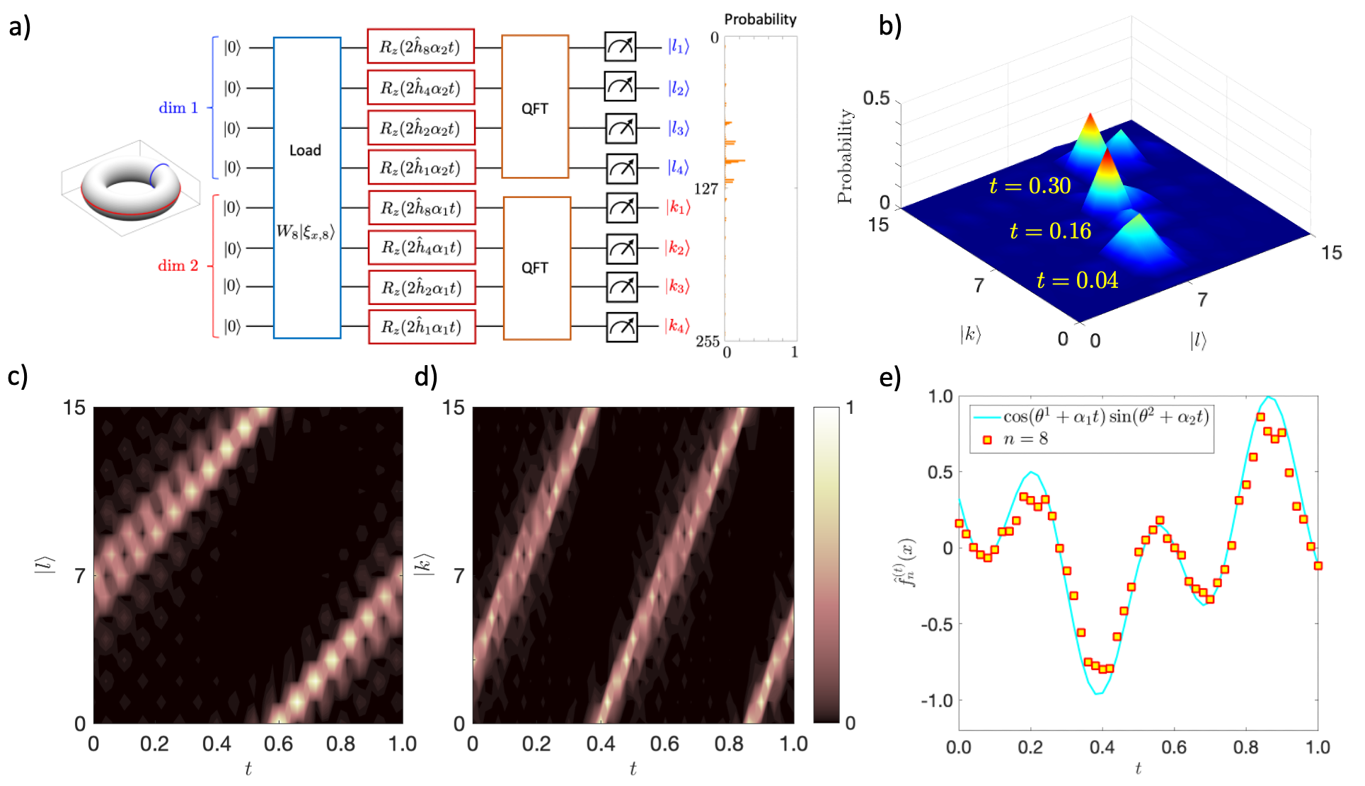
The two-dimensional case proceeds along similar lines as the one-dimensional example in Sec. IX.1, so we mainly focus on the points that are different from the one-dimensional example. The classical dynamical orbit on the 2-torus is now given by
where and are the frequency parameters and is the initial condition. We choose the (rationally independent) values and , leading to an ergodic flow on . We again seek to approximate the evolution of a bandlimited classical observable , in this case . The evolution of this observable is given by
To perform quantum simulation, we set the RKHA parameters as in Sec. IX.1, and use a total of cubits, which corresponds to 4 qubits allocated to each torus dimension. The quantum computational Hilbert space, , is thus 256-dimensional, and admits the tensor product factorization
| (79) |
For convenience in the notation, we will label the basis vectors for each of the factors in (79) as and , where and are 4-digit binary strings. Note that the factorization in (79) is compatible with the tensor product structure of the infinite-dimensional RKHA in (13), in the sense that each factor corresponds to the image space under a projection of the spaces in (13). See also Appendix B, and in particular (96). A similar tensor product structure applies for the quantum feature map, dynamical evolution, and QFT operators,
| (80) | ||||
so we can form the entire circuit by composing two 4-qubit circuits from the one-dimensional case; see Fig. 8(a) for an illustration. In (80), -superscripts and -subscripts denote maps inherited from the one-dimensional case.
As in the one-dimensional example of Sec. IX.1, all quantum states occurring in our scheme are pure, so we implement the circuit in Fig. 8(a) at the level of the vectors (normalized RKHS feature vectors), (initial state vectors), (Koopman-evolved state vectors), and (state vectors after application of the QFT). Note that the normalized feature vector associated with classical state takes the form
with and
See again Table 2 for an example of the ordering of the multi-index and its mapping to the computational basis in the case (the table would have 256 rows in the current example). We also note that our example has nonzero Walsh-Fourier expansion coefficients: , , , and for each torus dimension.
Figure 8(b) displays snapshots of the empirical joint probability distribution of the indices at representative evolution times , obtained from ensembles of measurements of the quantum computational PVM on the state represented by for the initial condition . The locality of the distributions is indicative of the fact that the quantum computing model successfully tracks the orbit of the underlying classical dynamical system. Figs. 8(d) and 8(d) show marginals of these distributions over the and index spaces as a function time , where periodic evolution at the generating frequencies and , respectively, is apparent.
In Fig. 8(e) we compare the approximate evolution of the observable computed from the same ensembles of quantum measurements against the true evolution . Despite the modest number of qubits allocated to each torus dimension, reproduces the quasiperiodic behavior of to an adequate degree of accuracy, with more pronounced errors occurring near the extrema of the true signal. As in the one-dimensional example of Fig. 6(d), we expect such discrepancies to rapidly diminish as the number of qubits increases. Similarly, from this example it becomes clear how one can generalize the dynamics to a torus of dimension .
X Experiments on the IBM Quantum System One

The circle rotation algorithm for qubits was also implemented on the IBM Quantum System One to demonstrate the readiness of QECD on a real NISQ device. This system has a quantum volume (an empirical metric that quantifies the capability and error rates of a quantum device) of 32. The corresponding program was again written in Qiskit (see Sec. IX), and then transpiled (translated) into a sequence of appropriate elementary gate operations acting on the physical superconducting qubits via microwave channels at the hardware level. No error correction was used in our simulation. As mentioned in Sec. VIII, the encoding of (complex) amplitudes that represent the feature vector associated with classical state in an -qubit quantum register can lead to an exponential growth of gates. To give a concrete example for : amplitude encoding using QuantumCircuit.initialize with no circuit optimization is transpiled into a sequence of 84 elementary quantum gates. This conversion results to 52 elementary gates for a higher transpiler optimization level of 2.
To circumvent this expensive amplitude encoding of classical data, it was shown in Sec. VIII that the initial state vector can also be obtained to any degree of accuracy with a circuit of size and depth . In the particular case (i.e., the point with canonical angle coordinates ), the encoding reduces to a uniform superposition state for -qubits, , which is obtained via Hadamard gates applied to the standard basis quantum state (see (76)). This step reduces the number of gates, and thus the circuit depth, significantly to 33 and 30 for the transpiler optimization levels 0 and 2, respectively. This depth is close to the quantum volume of the computer.
Figure 9 directly compares the results of an ideal Qiskit Aer simulator for and with an experiment on the IBM Quantum System One for the observable and an initial uniform superposition state (approximating ). Despite the noise caused by decoherence, the evolution of probability densities (Fig. 9(b)) and expectation values (Fig. 9(c)) obtained from the NISQ device remain consistent with the Qiskit simulation (Fig. 9(a,c)). The number of shots, which is limited to 8192 on the Quantum System One, was enhanced to by aggregating results from multiple jobs.
Unfortunately, increasing the number of qubits beyond led to noticeable degradation of the results on the quantum computer relative to the Qiskit simulations, despite our best efforts to manage noise and decoherence with the tools available to us. Still, to our knowledge, the results reported in this section constitute the first successful simulation of an observable of a classical dynamical system on a manifold by an actual NISQ device. We expect that as the coherence characteristics, error mitigation and/or circuit optimization schemes for quantum computation improve, the QECD framework presented in this paper will successfully scale to higher qubit numbers.
XI Summary and outlook
We have developed a framework for approximating the evolution of observables of a classical dynamical system by a finite-dimensional quantum system implementable on an actual quantum computer. The procedure, which we refer to as quantum embedding of classical dynamics (QECD), takes the classical system as an input, and passes through intermediate classical statistical, infinite-dimensional quantum mechanical, and finite-dimensional quantum mechanical (matrix-mechanical), representations, ultimately arriving at an -qubit quantum computational representation of the system. We have thus addressed the full pipeline starting from the classical dynamical system all the way to its experimental verification on a real quantum computer, the IBM Quantum System One.
For the class of dynamical systems under study (i.e., measure-preserving, ergodic dynamical systems with pure point spectra), QECD provides an exponential quantum advantage over classical computation, in the sense of being able to simulate a -dimensional Hilbert space of classical observables using circuits of size and depth . In addition, the quantum state encoding the initial classical quantum state is efficiently prepared, and predictions from the quantum computational system are extracted through projective measurement in the standard computational basis without requiring postprocessing techniques such as quantum state tomography.
One of the mathematical underpinnings of our approach is the theory of reproducing kernel Hilbert spaces (RKHSs). RKHS theory is widely used in kernel methods for machine learning, but was employed here to construct quantum mechanical analogs of feature maps that behave consistently under classical function evaluation and quantum mechanical expectation. A further foundational ingredient is the operator-theoretic description of dynamical systems, which utilizes linear Koopman operators to characterize the action of a (nonlinear) dynamical system on observables.
We described how QECD proceeds along two composite mappings, one taking state variables to density operators on an -qubit Hilbert space, , and another one taking classical observables to self-adjoint operators on . A key aspect of the resulting quantum system is a tensor product factorization of its Hamiltonian in terms of Walsh operators, yielding quantum circuits of low size and depth. In particular, it was shown that for an ergodic dynamical system with finitely-generated pure point spectrum, this results in a circuit of size and no cross-channel communication, implementing unitary Koopman evolution. The QECD framework also includes a state preparation stage of size , as well as a quantum Fourier transform (QFT) stage of size to enable information retrieval through measurement in the computational basis.
The scheme exhibits three types of approximation error, all of which can be controlled, as we have shown, in appropriate asymptotic limits:
-
1.
Finite-dimensional approximation errors due to projection of the infinite-dimensional quantum system on the RKHS to the finite-dimensional quantum computational system on . These errors vanish as , and the convergence is unconditional on the defining parameters of if idealized state preparation and measurement is employed (see Sec. V).
- 2.
-
3.
Monte Carlo errors associated with approximation of quantum mechanical expectations with a finite number of measurement shots (see Sec. VII.2). These errors vanish as the number of shots, , increases at fixed and .
We illustrated our approach with periodic and quasiperiodic dynamical systems on the circle and 2-torus, respectively, where many aspects of the quantum embedding of classical dynamics can be directly validated against closed-form solutions. Our numerical experiments were based on simulated quantum circuits of up to qubits, implemented using the Qiskit framework. In addition we demonstrated the ability of our framework to deal with a classical dynamical system on a real noisy quantum computer. The results demonstrated high-fidelity simulation of the evolution of classical observables through ensemble averages of independent quantum measurements. Our approach is straightforwardly generalizable to quasiperiodic dynamics of arbitrarily large intrinsic dimension through parallel composition of quantum circuits.
The work presented in this paper should be considered a first step, particularly given its focus on systems with pure point spectra. Applications of the procedure to mixing (chaotic) dynamical systems will invariably have to deal with the continuous spectrum of the Koopman operator, potentially generating quantum circuits of higher connectivity than for quasiperiodic dynamics. Studies in this direction are currently underway using RKHS-based spectral discretization approaches for Koopman operators [29] (see Sec. II C 2 in the SM), which are able to consistently approximate, in a spectral sense, measure-preserving, ergodic dynamical flows of arbitrary spectral character (pure point spectrum, mixed spectrum, and continuous spectrum) by unitary evolution groups with pure point spectra. A possible route to generalize QECD to this class of systems is to employ the scheme of Ref. [29] to first approximate the Koopman group on by a unitary evolution group on an RKHS with a discrete spectrum, and then apply the quantum computational techniques developed in this paper to simulate the discrete-spectrum system.
Another avenue of future research is to develop data-driven formulations of the present quantum embedding framework, using kernel methods to build orthonormal bases from dynamical trajectory data, and employ these bases to represent quantum mechanical states and observables [25] (see Sec. II in the SM [63]). This line of research should lead to a systematic development of quantum machine learning algorithms that can describe classical dynamical systems on NISQ devices. This comprises not only classification and regression tasks [36], but also the development of data-driven quantum algorithms for modeling nonlinear dynamics in high-dimensional phase spaces. A longer-term goal would be to explore applications of quantum mechanical methodologies to perform simulation and forecasting of real-world systems such as climate dynamics [78] and turbulent fluid flows [79].
Acknowledgements.
We wish to thank Sachin Bharadwaj for helpful discussions. We acknowledge the use of IBM Quantum services for this work. The views expressed are those of the authors, and do not reflect the official policy or position of IBM or the IBM Quantum team. In this paper we used ibmq_ehningen, which is one of the IBM Quantum Falcon Processors. We thank the Fraunhofer Gesellschaft (Germany) for support. D. Giannakis acknowledges support from the US National Science Foundation under grants 1842538 and DMS-1854383, the US Office of Naval Research under MURI grant N00014-19-1-242, and the US Department of Defense under Vannevar Bush Faculty Fellowship grant N00014-21-1-2946. The work of A. Ourmazd was supported by the US Department of Energy, Office of Science, Basic Energy Sciences under award DE-SC0002164 (underlying dynamical techniques), and by the US National Science Foundation under awards STC 1231306 (underlying data analytical techniques) and DBI-2029533 (underlying analytical models). P. Pfeffer is supported by the Deutsche Forschungsgemeinschaft with project SCHU 1410/30-1 and by the project “DeepTurb – Deep Learning in and of Turbulence” of the Carl Zeiss Foundation (Germany). J. Slawinska acknowledges support from the core funding of the Helsinki Institute for Information Technology (HIIT) and the Institute for Basic Sciences (IBS), Republic of Korea, under IBS-R028-D1.Appendix A Quantum mechanical representation of classical observables
In this appendix, we state various properties and results on the representation of classical observables by quantum mechanical operators employed in the main text.
A.1 Banach ∗-algebra structure of
The fact that the RKHA from Sec. III.2 is an abelian, unital, Banach ∗-algebra under pointwise multiplication of functions means that it has the following defining properties:
-
1.
is closed under pointwise multiplication of functions, i.e., the function with lies in whenever and lie in . Thus, is an algebra, and is clearly abelian since .
-
2.
is equipped with an antilinear involution operation given by complex conjugation of functions, i.e. . Thus, is also a ∗-algebra.
-
3.
There exists a constant such that for every the relationships
(81) hold. Thus, is a Banach ∗-algebra.
-
4.
The function equal everywhere to 1 lies in and satisfies for all . Thus, finally is also unital.
A.2 Injectivity of the map
We verify the assertion made in Section IV.3 that the map is injective on . For that, it is enough to show that if for , then . By definition of , implies that , or, equivalently
| (82) |
Expanding , and setting in (82), we get
However, because is real, we have , and since is nonzero we conclude that , and thus .
A.3 Consistency of representations based on the reproducing kernel Hilbert space
Recall the construction of the RKHS in Sec. IV.1. Even though is a strict subspace of the RKHA , the quantum feature map from (21) allows us to consistently recover all predictions made for classical observables obtained via the feature map of in (23), as we now describe.
First, observe that by definition of and , we have
| (83) |
where is the projector onto , defined in (28). As a result, if is a quantum mechanical observable whose range is included in (so that is well-defined as an operator on ), and whose nullspace includes the orthogonal complement in , we have
| (84) |
Indeed, since every observable in this class satisfies , using (83) and the cyclic property of the trace, we get
which verifies (84). Thus, for all observables satisfying
| (85) |
expectation values with respect to can be recovered from expectation values with respect to up to a constant scaling factor. For our purposes, this means that the quantum mechanical observables and obtained through the projections and of and from (24) and (25), respectively, satisfy (84).
As noted in Sec. IV.3.2, in order to reach consistency between classical function evaluation and quantum mechanical expectation, analogously to (31), we introduce the modified representation maps and in (29) to account for scaling errors. We reproduce the definitions here for convenience:
We define as the self-adjoint, diagonal operator satisfying the eigenvalue equation
| (86) |
where is the index set defined as
Note that by construction of , the numbers are strictly positive, and have the maximum value . Moreover, the attain their smallest value, , when , i.e., the multi-index has exactly one entry equal to and all other entries equal to 0. As a result, is an invertible operator with bounded inverse, satisfying
Since , we deduce that acts by inflating the expansion coefficients of elements of in the basis.
We then have:
Proposition 1.
The following classical–quantum consistency relation holds for every and :
Moreover, if is a real-valued observable in , we have
Proof.
Suppose that for some , and let , where is the multiplication operator by . Then, satisfies (85), and using (84), we get
| (87) |
Meanwhile, an application of (31) for gives
| (88) |
and combining (87) and (88) we arrive at
| (89) |
where . Since the basis vector was arbitrary, it follows by linearity that (89) holds for every . Setting, in particular, yields
which confirms the first claim of the proposition. The second claim, , follows similarly under the additional assumption that . ∎
A.4 Dynamics on the reproducing kernel Hilbert space
By construction, the RKHS is a Koopman-invariant subspace of , i.e., for all . As a result, we can define a generator with , a corresponding Koopman operator , and corresponding evolution maps on observables, , and states, analogously to the corresponding operators associated with . These operators satisfy the compatibility relations (cf. (35) and (37))
for every , , and , where is the map on observables in (29) and the quantum feature map in (21). In addition, using the consistency relations in Proposition 1 and (39), we get
| (90) | ||||
where was defined in (29), and the equalities in the second line hold for real-valued functions in . It follows from (90) that we can consistently represent the evolution of classical observables in (which is a dense subspace of ) by quantum mechanical evolution of observables in , even though is a non-dense subspace of .
Appendix B Walsh operator representation of the Koopman generator
Here, we lay out the calculation of the discrete Walsh transform of the spectral function of the Hamiltonian induced by the Koopman generator of a quasiperiodic dynamical system, defined in (60). In particular, we show that is expressible as a linear combination of Rademacher functions (without contributions from more general Walsh functions), leading to the factorization of in (61).
First, by (14) and (60), for any we have
| (91) |
where are integers in the set , defined uniquely by the property that the concatenated binary strings give the dyadic decomposition of ,
| (92) |
We can express the left-hand side of (92) in terms of Rademacher functions using (56), viz.
| (93) |
Meanwhile, setting and using again (56), the right-hand side of (92) becomes
| (94) |
Substituting for and in (92) using (93) and (94), respectively, we deduce that for each and
| (95) |
for all .
Observe now that for ,
where we used (95) to obtain the last line. Substituting the above in (91), we obtain
We therefore conclude that for a quasiperiodic system, the spectral function of the generator is expressible as a linear combination of Rademacher functions. Explicitly, we have
| (96) |
with
which is consistent with the factorization of the Hamiltonian in (61).
Appendix C Approximate diagonalization of observables using the quantum Fourier transform
In this appendix, we perform an analysis of approximate diagonalization of quantum mechanical observables induced at the quantum computational level from classical observables through the use of the QFT. In Appendices C.1 and C.2, we describe how such quantum mechanical observables become increasingly diagonal as the number of qubits increases, and provide explicit bounds verifying the approximate eigenvalue equation (72). In Appendix C.3, we show that quantum mechanical expectation values of the approximately diagonalized observables converge to the true expectation values in a limit of infinite qubit number and vanishing RKHA parameter . Appendices C.4 and C.5 contain proofs of two auxiliary lemmas, Lemma 2 and 4, which are stated in Appendices C.1 and C.3, respectively.
C.1 Approximate diagonalization in dimension
We begin with the one-dimensional case, , where . In this case, the index set in (17) becomes with , and the map in (69) reduces to the standard -qubit QFT, . We also recall that and are the parameters associated with the RKHA .
C.1.1 Diagonalization using the regular representation
Fixing , consider the regular representer (multiplication map) of basis vector , the associated quantum computational observable
and the Fourier-transformed observable
| (97) |
First, note that by definition of the projection , is the zero operator (and thus trivially diagonal) whenever . This is a manifestation of an effective “Nyquist limit” on the wavenumber of classical observables that can be resolved by the finite-dimensional system on . Here, we are interested in characterizing the behavior of in the “well-resolved” regime, . The following lemma provides a bound showing that (a) such well-resolved observables are approximately diagonal in the quantum computational basis ; and (b) the diagonal part approximately recovers the values of at particular points on the circle .
Lemma 2.
With the notation of (97), the observable satisfies
where , and is a residual obeying the bound
for a constant independent of , , , , , and .
A proof of Lemma 2 will be given in Appendix C.4. Using this basic result, we can derive error estimates for more general quantum mechanical observables than those induced by the individual basis functions .
First, note that the terms , , are bounded by a constant that depends on and (and diverges as either of these parameters tends to 0). Moreover, since , is bounded by a constant times . Thus, for every and there exists a constant such that for all ,
This means that we can simplify the estimate for in Lemma 2 to (the less precise) bound
| (98) |
Using (98), we estimate the square norm of the residual
as
giving
| (99) |
Thus, so long as , the norm of the residual converges to zero as , uniformly with respect to .
We next generalize to bandlimited observables, i.e., observables for which there exists such that , where the are the Fourier functions on , and the are complex expansion coefficients. We denote the vector space of such bandlimited observables on by . Note that is a dense subalgebra of , and is also a dense subalgebra of for any and (in the respective norms). In particular, viewed as an element of , can be equivalently expressed as , where .
By linearity, every such observable is represented at the quantum computational level by
and after application of the QFT by
| (100) |
Thus, using Lemma 2 and (99), we obtain
where the residual can be estimated as
We thus conclude that for bandlimited observables the off-diagonal residual vanishes as at fixed and , uniformly with respect to . For later convenience, we set
so that
| (101) |
Analogously to (99) we can bound the norm of the residual as
| (102) |
and we deduce that the residual vanishes as if .
Suppose now that is not bandlimited. Then, for any there exists such that the bandlimited observable satisfies
| (103) |
Defining
| (104) |
and by (100), we get
To bound the terms in the right-hand side of the last inequality, note first that the operators , , , , and all have unit norm. Using this fact, it follows that
Moreover, it follows from the reproducing property of that
Using these bounds and (101), we obtain
In particular, for large-enough we have
and thus
| (105) |
Since was arbitrary, we conclude that as , converges to 0, i.e., the matrix elements of the quantum mechanical observable are consistently approximated by the matrix elements of the diagonal observable associated with the values . Note that unlike the bandlimited case we do not have an explicit rate for this convergence.
Consider now the residual
| (106) |
In order to examine the asymptotic behavior of as , it is useful to view the spaces as a nested family of subspaces of the sequence space , i.e., . With this identification, is an orthonormal basis of , and is a bounded sequence in . According to (105), for any , this sequence satisfies
It then follows from standard Hilbert space results that as , converges to zero in the weak topology of . That is, for any , we have
| (107) |
where is the orthogonal projection of onto .
C.1.2 Diagonalization using the self-adjoint representation
Using the estimates obtained in Appendix C.1.1, we now derive approximate diagonalization results for the self-adjoint observables induced by the map in (25). For any , consider the self-adjoint observable with
| (108) |
where is defined in (104). Then, we have
and we can use the results of Appendix C.1.1 to bound the two terms in the last line. In particular, if is bandlimited, then it follows from (101) that
and for general ,
with the same notation as (105). Moreover, convergence results for the residual can be derived analogously to those for in Appendix C.1.1.
C.2 Approximate diagonalization in dimension
We can extend the results in Appendix C.1 to dimension by taking advantage of the tensor product structure of the RKHA on and the maps effecting the transformations from the classical to the quantum computational level. Following the notation of Sec. III.2, we will use -superscripts to distinguish vector spaces, vectors, and linear maps associated with the circle ; see, e.g., (13). With this notation, the representation map for dimension decomposes as , and similarly we have , , and with , , and , where we have assumed that the number of qubits is an integer multiple of . We also recall the definition of the tensor product QFT operator in (70), i.e.,
Given any tensor product element , we have
where
Meanwhile, for any binary string with associated evaluation point from (71) we have
Thus, for any two computational basis vectors and of with and we have
and we can use the results of Appendix C.1 to bound the right-hand side. In particular, it follows from (105) that converges to 0 as , so that is consistently approximated by a diagonal observable with eigenvalues equal to the values of at the points . Moreover, the residual is analogously to (102) if is bandlimited, and converges weakly to zero as increases in the sense of (107).
The extension to elements of which are not of tensor product form follows by linearity. We omit the details of these calculations in the interest of brevity.
Note now that for every , the spectrum of the corresponding multiplication operator consists precisely of the range of values of , i.e., [50]. In particular since the elements of are all continuous functions, has nonempty continuous spectrum, unless is constant. Define and as the diagonal operators satisfying
| (109) |
where is self-adjoint. The following theorem summarizes the properties of the quantum computational observables approximating and obtained in Appendices C.1 and C.2.
Theorem 3.
Let be arbitrary, and consider the operators and defined as in (104) and (108) for dimension . Consider also the diagonal operators in (109). Then, the following hold as .
-
a.
The matrix elements of converge to the matrix elements of .
-
b.
The matrix elements of converge to the matrix elements of .
-
c.
For each basis vector , the residuals and converge to zero weakly. Moreover, if is bandlimited, the convergence is strong and the norms of the residuals are .
-
d.
For every element there exists a sequence of eigenvalues of and a sequence of eigenvalues of such that and .
C.3 Convergence of quantum mechanical expectations
Thus far, we have established that every element of can be consistently approximated in a spectral sense by operators which are diagonal in the computational basis. By construction (see Theorem 3) the spectra of are subsets of the range of values of . As a result, quantum measurement of (which can be equivalently realized by measurement of the PVM associated with the computational basis as described in Sec. VII.2) yields outcomes consistent with values that takes on classical states in . While this is a desirable property to have, it does not in itself guarantee that the quantum mechanical measurements are consistent with the value of on the particular classical state that the system happen to have. Establishing this type of consistency is the goal of this appendix.
The convergence results that we derive will turn out to hold for a decreasing sequence of RKHA parameters , as opposed to fixed values in Appendices C.1 and C.2. Thus, in what follows, we will use the notation to make the dependence of the RKHAs on explicit. By construction, the spaces form an increasing nested family as decreases to 0; that is, for every and we have and . We also introduce explicit subscripts in our notation for the RKHSs and and the operators , , , and . subscripts will also be introduced in our notation for elements of , , and the associated operator spaces as appropriate.
As in Appendices C.1 and C.2, we consider first the one-dimensional case, , and an observable equal to a basis vector of . We define the diagonal operator with
analogously to (109), and also set with
We also define
| (110) |
as in (97). For any , we consider the quantum computational state and the state after application of the QFT,
| (111) |
We then have:
Lemma 4.
With notation as above, the limit of the expected difference between measurements of and on the state exists, and satisfies
A proof of Lemma 4 can be found in Appendix C.5. For our purposes, a key implication of the result is that while the bias in measuring (instead of ) need not vanish as , it can be made arbitrarily small for a suitable choice of . In particular, for any there exists such that for all we have , and thus
| (112) |
Since , the choice will suffice for (112) to hold.
Next, we consider bandlimited observables of the form . Let
| (113) |
be the corresponding quantum computational observable, and let be the diagonal observable approximating ,
| (114) |
Using Lemma 4 and following a similar approach as in Appendix C.1, we find
| (115) |
where
Again, for any , there exists such that
| (116) |
In this case, the choice is sufficient for the bound to hold.
To generalize to non-bandlimited observables, we must take into account the fact that the error bounds in (112) and (116) imply convergence on a decreasing sequence of RKHA parameters , as opposed to the diagonalization results in Appendix C.1 which hold for fixed . With that in mind, we consider a space of classical observables that contains the RKHAs for all admissible values of the parameters and . In particular, we consider observables in the Wiener algebra of , i.e., the space of functions with absolutely convergent Fourier series, which we denote here by . The Wiener algebra is a dense subalgebra of . Moreover, the RKHAs employed in this work are all dense subalgebras of . Thus, we have the following relationships between algebras of classical observables (which also hold in dimension ):
Suppose then that is an arbitrary element of , where the sum over converges uniformly on . Then, for any there exists such that for every the bandlimited observable satisfies
| (117) |
The bandlimited observable is an element of for any , with RKHA norm satisfying
| (118) |
We will also need the observable
as an intermediate approximation associated with the bias correction introduced in Sec. IV.4 and Appendix A.3 to take into account the projection from to . Here, is operator introduced in (86) and are its eigenvalues, where we have again used subscripts to make dependencies on that parameter explicit. We have
where
Note that to obtain the last result we used the fact that lies in the interval ; see Appendix A.3. In particular, as , converges to 0 since converges to 1 and tends to infinity. Proceeding as in the derivation of (118) to bound the sum , we arrive at
| (119) |
Next, define the quantum computational observable as
| (120) |
where , and are operators defined as in (110). Define also the diagonal observable
| (121) |
Letting be an arbitrary point in , defining the quantum state as in (111), and using (117) and (119) we get
We can now bound the second, third, and fourth terms in the right-hand side of the last inequality. In particular, it follows by applying Proposition 1 to the observable that
Then, using the above in conjunction with the fact that , it follows that for any there exists such that for all we have, simultaneously,
| (122) |
and thus
Since was arbitrary, we conclude that there exists a decreasing sequence of RKHA parameters such that the quantum mechanical expectation converges to the classical value in the iterated limit of (infinite bandwidth) after (infinite qubits), and the convergence is uniform with respect to .
Having established this convergence result in dimension , we can extend it to higher dimensions using tensor product arguments analogous to those in Appendix C.2. It is also straightforward to derive analogous results using the symmetrized map , inducing the self-adjoint quantum computational observable (cf. (120))
and the diagonal observable
| (123) |
We do not reproduce the details of these analyses in the interest of brevity. The following theorem summarizes the asymptotic convergence of our approach in these settings.
Theorem 5.
Let be a classical observable in the Wiener algebra of . For , , and , define the bandlimited observable and the corresponding diagonal quantum mechanical observables and from (121) and (123), respectively. Then, there exists a sequence , decreasing to 0, such that for any ,
uniformly with respect to .
The fact that quantum states at the quantum computational level evolve compatibly with the underlying classical dynamics, i.e., , leads to the following corollary of Theorem 5, which establishes the asymptotic consistency of QECD in simulating the evolution of classical observables.
Corollary 6.
With the notation of Theorem 5 and for any , let with
be the function representing the expected value of the time- simulation of by the quantum computer, given initial conditions . Then,
where the convergence is uniform with respect to and in compact sets. Moreover, if is real-valued, the analogous result holds for
Before closing this section, we note that while the convergence results in Theorem 5 and Corollary 6 hold for observables in the Wiener algebra with absolutely convergent Fourier series, the fact that is a dense subspace of means that any observable can be approximated to arbitrarily high precision in uniform norm by an observable , whose dynamical evolution can in turn be simulated to arbitrarily high precision using the quantum compiler as established in Corollary 6. The function may be constructed by several means available from signal processing, e.g., by convolution of by an appropriate smoothing kernel. A detailed study of this topic is beyond the scope of the present work.
C.4 Proof of Lemma 2
Using the definition of the map in (58) and the QFT in (68), we get
leading to
Therefore, the operator has the matrix elements
where
Observe now that if , then . Therefore, since whenever , we get
Thus, defining
and
we get
Note that we used standard properties of discrete Fourier transforms to arrive at the last line. It then follows by definition of the basis vectors and gridpoints that
as claimed in the statement of the lemma.
We now proceed to bound the remainder , assuming, for now, that . Letting , we have
| (124) |
where
Next, to bound the term, consider the function . Since , is strictly concave on the positive real line. Thus, for and , we have
| (125) |
Consider also the function on the interval with . The function is strictly convex, so
Therefore, for and , we obtain
| (126) |
Note that we have used (125) and the fact that (which follows from the same equation).
C.5 Proof of Lemma 4
We have
By the results in Sec. V and Appendix A, it follows that
| (130) |
where we recall the definition of the index set ,
Moreover, we have
In the above, the function can be expressed as
As , the summation in the parentheses in the last line converges to a continuous Fourier transform,
As a result, we have
and upon evaluation at ,
| (131) |
Therefore, combining (130) and (131), we obtain
and thus
Note now that for fixed , the largest value of over occurs for . That is, we have
so that
proving the lemma. ∎
References
- Feynman [1982] R. P. Feynman, Simulating physics with computers, Int. J. Theor. Phys. 21, 467 (1982).
- Lloyd [1996] S. Lloyd, Univeral quantum simulators, Science 273, 1073 (1996).
- Berry et al. [2007] D. W. Berry, G. Ahokas, R. Cleve, and B. C. Sanders, Efficient quantum algorithms for simulating sparse Hamiltonians, Commun. Math. Phys. 270, 359 (2007).
- Barnett [2009] S. Barnett, Quantum Information, Oxford Master Series in Atomic, Optical and Laser Physics (Oxford University Press, Oxford, 2009).
- Nielsen and Chuang [2010] M. A. Nielsen and I. L. Chuang, Quantum Computation and Quantum Information (Cambridge University Press, Cambridge, UK, 2010).
- Preskill [2018] J. Preskill, Quantum computing in the NISQ era and beyond, Quantum 2, 79 (2018).
- Deutsch [2020] I. H. Deutsch, Harnessing the power of the second quantum revolution, Phys. Rev. X Quantum 1, 020101 (2020).
- Grover [2001] L. K. Grover, From Schrödinger’s equation to quantum search algorithm, Am. J. Phys. 69, 769 (2001).
- Arute et al. [2019] F. Arute, K. Arya, R. Babbush, D. Bacon, et al., Quantum supremacy using a programmable superconducting processor, Nature 574, 505 (2019).
- Zhou et al. [2020] Y. Zhou, E. M. Stoudenmire, and X. Waintal, What limits the simulation of quantum computers?, Phys. Rev. X 10, 041038 (2020).
- Meyer [2002] D. A. Meyer, Quantum computing classical physics, Phil. Trans. R. Soc. A 360, 395 (2002).
- Benenti et al. [2001] G. Benenti, G. Casati, S. Montangero, and D. L. Shepelyansky, Efficient quantum computing of complex dynamics, Phys. Rev. Lett. 87, 227901 (2001).
- Leyton and Osborne [2008] S. K. Leyton and T. J. Osborne, A quantum algorithm to solve nonlinear differential equations (2008), arXiv:0812.4423 .
- Giannakis [2019a] D. Giannakis, Quantum mechanics and data assimilation, Phys. Rev. E 100, 032207 (2019a).
- Joseph [2020] I. Joseph, Koopman-von Neumann approach to quantum simulation of nonlinear classical dynamics, Phys. Rev. Research 2, 043102 (2020).
- Bharadwaj and Sreenivasan [2020] S. Bharadwaj and K. R. Sreenivasan, Quantum computation of fluid dynamics, Indian Acad. Sci. Conf. Ser. 3, 77 (2020).
- Gaitan [2020] F. Gaitan, Finding flows of a Navier–Stokes fluid through quantum computing, npj Quantum Inf. 6, 61 (2020).
- Mezzacapo et al. [2015] A. Mezzacapo, M. Sanz, L. Lamata, I. Egusquiza, S. Succi, and E. Solano, Quantum simulator for transport phenomena in fluid flows, Sci. Rep. 5, 13153 (2015).
- Lubasch et al. [2020] M. Lubasch, J. Joo, P. Moinier, M. Kiffner, and D. Jacksch, Variational quantum algorithms for nonlinear problems, Phys. Rev. A 101, 010301(R) (2020).
- Elliot and Gu [2018] T. J. Elliot and M. Gu, Superior memory efficiency of quantum devices for the simulation of continuous-time stochastic processes, npj Quantum Inf. 4, 18 (2018).
- Elliott et al. [2020] T. J. Elliott, C. Yang, F. C. Binder, A. J. P. G. Garner, J. Thompson, and M. Gu, Extreme dimensionality reduction with quantum modeling, Phys. Rev. Lett. 125, 260501 (2020).
- Berry et al. [2015] T. Berry, D. Giannakis, and J. Harlim, Nonparametric forecasting of low-dimensional dynamical systems, Phys. Rev. E. 91, 032915 (2015).
- Giannakis et al. [2015] D. Giannakis, J. Slawinska, and Z. Zhao, Spatiotemporal feature extraction with data-driven Koopman operators, J. Mach. Learn. Res. Proceedings 44, 103 (2015).
- Kawahara [2016] Y. Kawahara, Dynamic mode decomposition with reproducing kernels for Koopman spectral analysis, in Advances in Neural Information Processing Systems (Curran Associates, 2016) pp. 911–919.
- Giannakis [2019b] D. Giannakis, Data-driven spectral decomposition and forecasting of ergodic dynamical systems, Appl. Comput. Harmon. Anal. 62, 338 (2019b).
- Berry et al. [2020] T. Berry, D. Giannakis, and J. Harlim, Bridging data science and dynamical systems theory, Notices Amer. Math. Soc. 67, 1336 (2020).
- Das and Giannakis [2020] S. Das and D. Giannakis, Koopman spectra in reproducing kernel Hilbert spaces, Appl. Comput. Harmon. Anal. 49, 573 (2020).
- Klus et al. [2020] S. Klus, F. Nüske, S. Peitz, J.-H. Niemann, C. Clementi, and C. Schütte, Data-driven approximation of the Koopman generator: Model reduction, system identification, and control, Phys. D 406, 132416 (2020).
- Das et al. [2021] S. Das, D. Giannakis, and J. Slawinska, Reproducing kernel Hilbert space quantification of unitary evolution groups, Appl. Comput. Harmon. Anal. 54, 75 (2021).
- Schuld et al. [2015] M. Schuld, I. Sinayskiy, and F. Petruccione, An introduction to quantum machine learning, Contemp. Phys. 56, 172 (2015).
- Biamonte et al. [2017] J. Biamonte, P. Wittek, N. Pancotti, N. Wiebe, and S. Lloyd, Quantum machine learning, Nature 549, 195 (2017).
- Ciliberto et al. [2018] C. Ciliberto, M. Herbster, A. D. Ialongo, M. Pontil, A. Rocchetto, S. Severini, and L. Wossnig, Quantum machine learning: A classical perspective, Proc. R. Soc. A 474, 20170551 (2018).
- Schuld and Killoran [2019] M. Schuld and N. Killoran, Quantum machine learning in feature Hilbert spaces, Phys. Rev. Lett. 122, 040504 (2019).
- Havlíček et al. [2019] V. Havlíček, A. D. Córcoles, K. Temme, A. W. Harrow, A. Kandala, J. M. Chow, and J. M. Gambetta, Supervised learning with quantum-enhanced feature spaces, Nature 567, 209 (2019).
- Blank et al. [2020] C. Blank, D. K. Park, J.-K. K. Rhee, and F. Petruccione, Quantum classifier with tailored quantum kernel, npj Quantum Inf. 6, 41 (2020).
- Schuld [2021] M. Schuld, Supervised quantum machine learning models are kernel methods (2021), arXiv:2101.11020 .
- Dellnitz and Junge [1999] M. Dellnitz and O. Junge, On the approximation of complicated dynamical behavior, SIAM J. Numer. Anal. 36, 491 (1999).
- Dellnitz and Froyland [2000] M. Dellnitz and G. Froyland, On the isolated spectrum of the Perron–Frobenius operator, Nonlinearity 13, 1171 (2000).
- Mezić [2005] I. Mezić, Spectral properties of dynamical systems, model reduction and decompositions, Nonlinear Dyn. 41, 309 (2005).
- Rowley et al. [2009] C. W. Rowley, I. Mezić, S. Bagheri, P. Schlatter, and D. S. Henningson, Spectral analysis of nonlinear flows, J. Fluid Mech. 641, 115 (2009).
- Williams et al. [2015] M. O. Williams, I. G. Kevrekidis, and C. W. Rowley, A data-driven approximation of the Koopman operator: Extending dynamic mode decomposition, J. Nonlinear Sci. 25, 1307 (2015).
- Klus and Koltai [2016] S. Klus and C. Koltai, P. Schütte, On the numerical approximation of the Perron-Frobenius and Koopman operator, J. Comput. Dyn. 3, 51 (2016).
- Brunton et al. [2017] S. L. Brunton, B. W. Brunton, J. L. Proctor, E. Kaiser, and J. N. Kutz, Chaos as an intermittently forced linear system, Nat. Commun. 8, 10.1038/s41467-017-00030-8 (2017).
- Baladi [2000] V. Baladi, Positive Transfer Operators and Decay of Correlations, Advanced Series in Nonlinear Dynamics, Vol. 16 (World scientific, Singapore, 2000).
- Eisner et al. [2015] T. Eisner, B. Farkas, M. Haase, and R. Nagel, Operator Theoretic Aspects of Ergodic Theory, Graduate Texts in Mathematics, Vol. 272 (Springer, 2015).
- Ferreira and Menegatto [2013] J. C. Ferreira and V. A. Menegatto, Positive definiteness, reproducing kernel Hilbert spaces, and beyond, Ann. Funct. Anal. 4, 64 (2013).
- Paulsen and Raghupathi [2016] V. I. Paulsen and M. Raghupathi, An Introduction to the Theory of Reproducing Kernel Hilbert Spaces, Cambridge Studies in Advanced Mathematics, Vol. 152 (Cambridge University Press, Cambridge, 2016).
- Feichtinger et al. [2007] H. G. Feichtinger, S. S. Pandey, and T. Werther, Minimal norm interpolation in harmonic Hilbert spaces and Wiener amalgam spaces on locally compact abelian groups, J. Math. Kuoto Univ. 47, 65 (2007).
- Kuznetsova and Molitor-Braun [2012] Y. Kuznetsova and C. Molitor-Braun, Harmonic analysis of weighted -algebras, Expo. Math. 30, 124 (2012).
- Das and Giannakis [2019] S. Das and D. Giannakis, On harmmonic Hilbert spaces on compact abelian groups (2019), arXiv:1912.11664 .
- Mauro [2002] D. Mauro, On Koopman–von Neumann waves, Int. J. Mod. Phys. A 17, 1301 (2002).
- Klein [2018] U. Klein, From Koopman–von Neumann theory to quantum theory, Quantum Stud.: Math. Found. 5, 219 (2018).
- Bondar et al. [2019] D. I. Bondar, F. Gay-Balmaz, and C. Tronci, Koopman wavefunctions and classical–quantum correlation dynamics, Proc. Roy. Soc. A 475, 20180879 (2019).
- Morgan [2020] P. Morgan, An algebraic approach to Koopman classical mechanics, Ann. Phys. 414, 168090 (2020).
- Giannakis [2020] D. Giannakis, Quantum dynamics of the classical harmonic oscillator, J. Math. Phys. 62, 042701 (2020).
- Welch et al. [2014] J. Welch, D. Greenbaum, S. Mostame, and A. Aspuru-Guzik, Efficient quantum circuits for diagonal unitaries without ancillas, New J. Phys. 16, 033040 (2014).
- Benedetti et al. [2019] M. Benedetti, E. Lloyd, S. Sack, and M. Fiorentini, Parametrized quantum circuits as machine learning models, Quantum Sci. Technol. 4, 043001 (2019).
- Marković and Grollier [2020] D. Marković and J. Grollier, Quantum neuromorphic computing, Appl. Phys. Lett. 117, 150501 (2020).
- Coppersmith [1994] D. Coppersmith, An Approximate Fourier Transform Useful in Quantum Factoring, Tech. Rep. (IBM, 1994) arXiv:quant-ph/0201067 .
- Moore and Nilsson [2001] C. Moore and M. Nilsson, Parallel computation and quantum codes, SIAM J. Comput. 31, 799 (2001).
- Anis et al. [2021] M. S. Anis, H. Abraham, and et al., Qiskit: An open-source framework for quantum computing (2021).
- Abraham et al. [2019] H. Abraham et al., Qiskit: An open-source framework for quantum computing (2019).
- Giannakis et al. [2021] D. Giannakis, A. Ourmazd, P. Pfeffer, J. Schumacher, and J. Slawinska, Supplementary information – embedding classical dynamics in a quantum computer (2021).
- Koopman [1931] B. O. Koopman, Hamiltonian systems and transformation in Hilbert space, Proc. Natl. Acad. Sci. 17, 315 (1931).
- Koopman and von Neumann [1931] B. O. Koopman and J. von Neumann, Dynamical systems of continuous spectra, Proc. Natl. Acad. Sci. 18, 255 (1931).
- Wang et al. [2020] X. Wang, J. Slawinska, and D. Giannakis, Extended-range statistical ENSO prediction through operator-theoretic techniques for nonlinear dynamics, Sci. Rep. 10, 2636 (2020).
- Schölkopf et al. [1998] B. Schölkopf, A. Smola, and K. Müller, Nonlinear component analysis as a kernel eigenvalue problem, Neural Comput. 10, 1299 (1998).
- Peres [2002] A. Peres, Quantum Theory: Concepts and Methods, Fundamental Theories of Physics, Vol. 72 (Kluwer Academic Publishers, New York, 2002).
- Grebogi et al. [1985] C. Grebogi, E. Ott, and J. A. York, Attractors on an -torus: Quasiperiodicity versus chaos, Phys. D 15, 354 (1985).
- Ecke et al. [1991] R. E. Ecke, R. Mainieri, and T. S. Sullivan, Universality in quasiperiodic Rayleigh-bénard convection, Phys. Rev. A 44, 8103 (1991).
- Weixing et al. [1993] D. Weixing, H. Wei, W. Xiagong, and C. X. Yu, Quasiperiodic transition to chaos in a plasma, Phys. Rev. E 70, 170 (1993).
- Kalogirou et al. [2015] A. Kalogirou, E. E. Keaveny, and D. T. Papageorgiou, An in-depth numerical study of the two-dimensional Kuramoto-Sivashinsky equation, Proc. R. Soc. A 471, 20140932 (2015).
- Budisić et al. [2012] M. Budisić, R. Mohr, and I. Mezić, Applied Koopmanism, Chaos 22, 047510 (2012).
- Note [1] This implies (i) , (ii) , and (iii) for all and .
- Stone [1932] M. H. Stone, On one-parameter unitary groups in Hilbert space, Ann. Math 33, 643 (1932).
- Cucker and Smale [2001] F. Cucker and S. Smale, On the mathematical foundations of learning, Bull. Amer. Math. Soc. 39, 1 (2001).
- Note [2] The qubit ordering in Qiskit is reverse to that in most textbooks on quantum computing.
- Slawinska et al. [2019] J. Slawinska, A. Ourmazd, and D. Giannakis, A quantum mechanical approach for data assimilation in climate dynamics, in Workshop on “Climate Change: How Can AI Help?”, 36th International Conference on Machine Learning (ICML)” (Long Beach, California, 2019).
- Giannakis et al. [2018] D. Giannakis, A. Kolchinskaya, D. Krasnov, and J. Schumacher, Koopman analysis of the long-term evolution in a turbulent convection cell, J. Fluid Mech. 847, 735 (2018).
- Wermer [1954] J. Wermer, On a class of normed rings, Ark. Mat. 2, 537 (1954).
- Brandenburg [1975] L. Brandenburg, On identifying the maximal ideals in Banach algebras, J. Math. Anal. App. 50, 489 (1975).
- Feichtinger [1979] H. G. Feichtinger, Gewichtsfunktionen auf lokalkompakten Gruppen, Sitzber. d. österr. Akad. Wiss. 188, 451 (1979).
- Gröchenig [2007] K. Gröchenig, Weight functions in time-frequency analysis, in Pseudodifferential Operators: Partial Differential Equations and Time-Frequency Analysis, Fields Inst. Commun., Vol. 52, edited by L. Rodino et al. (American Mathematical Society, Providence, 2007) pp. 343–366.