October 1, 2022
Embedding and correlation tensor for XRP transaction networks
Abstract
Cryptoassets are growing rapidly worldwide. One of the large cap cryptoassets is XRP. In this article, we focus on analyzing transaction data for the 2017–2018 period that consist one of the significant XRP market price bursts. We construct weekly weighted directed networks of XRP transactions. These weekly networks are embedded on continuous vector space using a network embedding technique that encodes structural regularities present in the network structure in terms of node vectors. Using a suitable time window we calculate a correlation tensor. A double singular value decomposition of the correlation tensor provides key insights about the system. The significance of the correlation tensor is captured using a randomized correlation tensor. We present a detailed dependence of correlation tensor on model parameters.
1 Introduction
Cryptoassets are digital assets, which use cryptography and depend on distributed ledger technology, also known as blockchain. The cryptomarket consists of many cryptoassets, namely, Bitcoin, Etherium, and XRP etc. Recently, we have witnessed increase in investor attention on cryptoassets. However, the risk for investing in cryptoassets is generally high due to the high volatility of their market price. Moreover, as the growing cryptoassets market can disrupt the financial market and the possibility of money laundering, policymakers in different countries have already started enacting regulations for its use. The cryptoassets have also attracted attention from researchers of different fields to study the fluctuation in price, transaction patterns of users, and efficiency, robustness of the underlying blockchain technology. While there are many studies on Bitcoin and Etherium [1, 2, 3], there are very few studies on XRP [4, 5]. In this work, we focus on analyzing XRP transactions.
Time series analysis comprises different methods to characterize and extract crucial insights for various time series data in the stock markets [6, 7, 8], foreign exchange markets [9, 10] or even in medical recordings [11]. The cross correlation is one of the popular methods to analyze time series data [6, 7, 8, 11]. The simplest way to measure correlation is the Pearson correlation, which is defined for a pair of variables as . Here is the no of observations or the length of the time series. The mean and standard deviations of and are represented as , and . The applications of cross correlation method with random matrix theory on time series data have provided valuable insights for different systems.
Recently, inspired by the cross correlation analysis of time series, A. Chakraborty et al. have developed a method of correlation tensor spectra for dynamical XRP transaction networks [12] to capture price burst. Following this article, we show the details of the embedding method for weekly directed weighted XRP networks. Using the embedded node vectors, we calculate the correlation tensors for XRP transaction netwokrs. The significance of the elements of the correlation tensor and its spectra is shown by comparing with randomized correlation tensor. Furthermore, We uncover the dependence of the correlation tensor on various model parameters, such as the embedding dimension, and the time window in detail.
2 Data description
Our data consist of the direct transactions between different XRP wallets from October 2, 2017 to March 4, 2018. The dataset was recorded as ledger data using the Ripple Transaction Protocol. We divided this dataset into groups based on different weeks. We constructed a weekly directed weighted network of XRP transactions by aggregating all the transactions for a week. In this network, XRP wallets are the nodes and a link represents the flow of XRP from a source wallet to a destination wallet. The total amount of weekly XRP flow between a pair of wallets represents the link weight. The XRP transactions data were collected from the ripple data API at https://xrpl.org/data-api.html.
3 Embedding of XRP transaction networks
Network embedding is a technique for representation of a network in low dimensional vector space by preserving key network features, which is useful for downstream tasks, such as network visualization, network analysis, link predication etc. The DeepWalk [13] and node2vec [14] are the two well-known methods for network embedding with structural information. We briefly describe these two methods below.
3.1 DeepWalk
Following the natural language models [15], B. Perozzi et al. developed the DeepWalk algorithm [13], which maps each node of a network as a vector in a dimensional continuous space by modeling a set of truncated random walks. The algorithm encodes the network community structure into a vector representation of the nodes. Many short random walk are used to compute local community structure information efficiently. These walks correspond to short sentences in language modeling. More specifically, it uses many random walks of length from each node. For each node, the algorithm generates a random walk of length and uses it to update the SkipGram algorithm in accordance with an objective function. The objective function maximizes the co-occurrence probability with other nodes present in the short random walk sequence. For a mapping function , the objective function can be written as
| (1) |
where is the window size, is the node set generated by the random walks from and represents the on the vector space. The algorithm uses the hierarchical softmax [16] to speed up the optimization procedure.
3.2 node2vec
A. Grover et al. further generalized the Deepwalk method by modifying the random walks as second order biased random walks. This method can encode more complex regularities of the network, such as functional relationships into the vector representation of nodes, depending on the tuning parameters and for the walks . It becomes equivalent to DeepWalk method when .
Here we have used node2vec with to embed weighted directed weekly XRP transactions networks.
4 Correlation tensor from embedded XRP transaction networks

We embed each of these weeekly weighted directed networks using node2vec with . It gives vector representations for each node , where ; ; . Here represents the dimension of the embedding space and is the total number of nodes in the -th week network. We identify that there are nodes that carry out at least one transaction each week. We call these nodes, regular nodes. The regular nodes play key role in the XRP trading market as they carry out frequent and consistent transactions. Considering the embedded vectors of regular nodes , where , we calculate the correlation tensor as follows
| (2) |
where is taken over weekly networks. The and represents mean and standard deviation of over a time window of networks.
The correlation tensor has elements. To uncover the crucial insights from the correlation tensor, we use a double singular value decomposition (SVD) technique as follows:
As a first step, we conduct the diagonalization of in terms of -index
| (3) |
and as a second step, we perform the digonalization in terms of -index successively
| (4) |
Then, using Eq. 3 and Eq. 4 we have
| (5) |
Here represents the generalized real and positive singular values as the correlation tensor is real.
5 Results

We show the daily XRP/USD price between 2017, May 18 and 2022 October 13 in Fig. 1. The period consists several peaks of XRP/USD price. The most extraordinary rise and fall of XRP/USD price is observed around January 2018. So we focus our study between October 2, 2017 and March 4, 2018, which covers 22 weeks.
We construct a weekly network of XRP transactions by aggregating all the transactions among the wallets. Wallets are the node and a directed link is formed between a source wallet and a destination wallet. The total flow of XRP between two wallets represents the link-weight. We show the temporal variation of number of nodes, links and value of total link-weight in Fig. 2. We observe that the number of nodes in the weekly networks increases rapidly around December 2017 and started decreasing again from the second week of January 2018, as shown in Fig. 2 (a). Fig. 2 (b) shows that the number of links per node, also known as average in-degree or out-degree decreases from to during October, 2017-March 04, 2018. The variation of the total transaction volume which represents total link-weight in weekly networks, is shown in Fig. 2 (c). We observe three sudden peaks in the transactions volume, which may be associated with the XRP price bubble during January 2018.
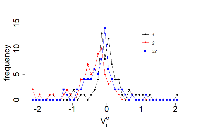
The distributions for the components of the node vector for all regular nodes for three different values of are shown in Fig. 3 for the week 2017, October 02 to October 08. The distributions have a peak indicating that the nodes are not embedded randomly on the vector space but capture the regularities of the network.


We calculate auto-correlation for each component of the node vectors . The auto-correlation is defined as the Pearson correlation for a time series as a function of the time lag. The auto-correlation function for the different components for different values of , and is shown in Fig 4. It is evident that the components do not have any significant auto correlation.
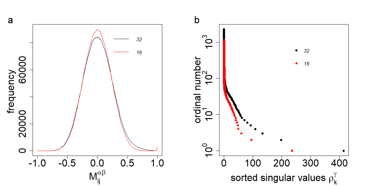
We show the distributions for the elements of correlation tensors with different time windows in Fig. 5 (a). It is observed that the peak of the distribution becomes sharper as we increase the time window and approaches a saturation form. We also notice that if we consider the time window , the distribution appears with two more peaks at due to high noise. The correlation tensor contains more noise as we decrease the values of the time window . The singular values of correlation tensors with different time windows is shown in Fig. 5 (b). We observe that the largest singular value decreases as the time window increases.
To understand the significance of the correlation tensor, we need a reference correlation tensor. We consider the following null hypothesis for the reference correlation tensor. We assign uniform random numbers between to the components of the embedding node vectors. We then calculate the randomized correlation tensor from these components of the embedding node vectors. We compare the distributions for the elements of the empirical correlation tensor and randomized correlation tensor in Fig. 6 (a). We observe that the distribution for the randomized correlation tensor has a higher peak and it is symmetric around zero. The distribution for the empirical correlation tensor is asymmetric and has a positive mean.
We further compare the singular values of the empirical and randomized correlation tensors in Fig. 6 (b). We observe that the largest singular value of the empirical correlation tensor lies significantly beyond the largest singular value of the randomized correlation tensor.
We show the dependence of the correlation tensor on the dimension of embedding vector space in Fig. 7. The distribution of the elements of the correlation tensor becomes narrower as we increase the dimension, as shown in Fig. 7 (a). The corresponding singular values of the correlation tensors are shown in Fig. 7 (b). The largest singular value increases as we embed the weekly networks in a higher dimension.
6 Conclusion
We have analyzed the XRP transactions focusing during the period between October, 02, 2017 and March 04, 2018. During this period, a significant price burst of XRP was observed. We have constructed weekly directed networks from XRP transactions. We have embedded these weekly networks in vector space, which capture the community structure information of the weekly networks in the embedded node vectors. The correlation tensor and its spectra are calculated using different time windows. It is observed that the the correlation tensor is sensitive to the time window. Lower the values of time window, it contains more noise. As we increase the time window, the distribution of the elements of correlation tensor approaches to the fixed form. The results were compared with randomized counterpart. It is observed that the distribution for the elements of empirical correlation tensor differs significantly. The largest singular value of the empirical correlation tensor appears well above the largest singular value of the randomized correlation tensor. Furthermore, we have presented the dependence of the correlation tensor on model parameters in detail.
This method is very useful and can capture valuable insights about the dynamical properties of the XRP transaction networks [12]. The embedding of the nodes encodes the community structure in the node vectors. The correlation is calculated between the components of the regular node vectors. Therefore, the spectra of the correlation tensors can capture whether there is a change in the community structure of the XRP transaction networks.
Acknowledgements
We thank the members of the Kyoto Univ.- RIKEN blockchain study group for discussions. YI acknowledges the grant, ”University Blockchain Research Initiative”, provided by Ripple, Inc. to Kyoto University for partial support to this work.
References
- [1] J. Wu, J. Liu, Y. Zhao, and Z. Zheng, J. Netw. Comput. Appl. 190, 103139 (2021).
- [2] D. Kondor, M. Pósfai, I. Csabai, and G. Vattay, PloS one 9, e86197 (2014).
- [3] S. Ferretti, and G. D’Angelo, Concurr. Comput. Pract. Exp. 32, e5493 (2020).
- [4] Y. Ikeda, In Digital Designs for Money,Markets, and Social Dilemmas, 203–220 (Springer, 2022).
- [5] H. Aoyama, Y. Fujiwara, Y. Hidaka, and Y. Ikeda, PloS one 17, e0273068 (2022).
- [6] L. Laloux, P. Cizeau, J. P. Bouchaud, and M Potters, PRL, 83, 1467 (1999).
- [7] V. Plerou, P. Gopikrishnan, B. Rosenow, L. A. N. Amaral, and H. E. Stanley, PRL 83, 1471 (1999).
- [8] V. Plerou et al., PRE 65, 066126 (2002).
- [9] A. Chakraborty, S. Easwaran, and S. Sinha, Phys. A: Stat. Mech. its Appl. 509, 599 (2018).
- [10] A. Chakraborty, S. Easwaran, and S. Sinha, Acta Phys. Polonica A 138, 105 (2020).
- [11] K. Schindler, H. Leung, C. E. Elger, and K. Lehnertz, Brain 130, 65–77 (2007).
- [12] A. Chakraborty, T. Hatsuda, and Y. Ikeda Scientific Reports 13, 4718 (2023).
- [13] B. Perozzi, R. Al-Rfou, and S. Skiena, Proc. ACM SIGKDD int. conf. Know. dis. and data mining 20, 701 (2014).
- [14] A. Grover, and J. Leskovec, Proc. ACM SIGKDD int. conf. on Know. dis. and data mining 22 855 (2016).
- [15] R. Collobert, and J. Weston, Proc. Int. Conf. Mach. Learn. 25, 160 (2008).
- [16] A. Mnih, and G. E. Hinton, Adv. neur. info. proc, sys. 21 (2009).