Embedded solitons in second-harmonic-generating lattices

For $\epsilon\gg 1$, equations (3a) and (3b) may be approximated by their continuous counterparts:

The variational approximation, which may be efficiently used to construct soliton-like solutions of discrete equations [22, 23, 24], does not apply to Eqs. (3a), (3b), as well as to their continuous-limit counterparts (8a), (8b), because these systems cannot be derived from Lagrangians, except for the case of $\gamma_{1}=2\gamma_{2}$ (numerical results are produced below for the case of $\gamma_{1}=\gamma_{2}$, when the Lagrangian representation is not available). Nevertheless, it is possible to apply the averaging method [21], which uses an adopted ansatz, such as the one introduced below in Eq. (9), as an “optimal” approximate localized solution of Eqs. (3a), (3b). The averaging method amounts to the variational one if the underlying equation is Lagrangian [21].

Motivated by the example of the exact embedded soliton found in Ref. [9], we assume that localized solutions of Eqs. (8a) and (8b) may be approximated by

Following the averaging method, we substitute the ansatz in Eqs. (8a), (8b), multiply the first equation by $\partial U/\partial A$ and the second one by $\partial V/\partial B$, and integrate the resulting expressions over $-\infty<x<+\infty$, to derive the following relations between parameters of the ansatz:

Because of the possible presence of the nonvanishing tail in the SH component, we seek for solutions in the form of

where $V_{0}$ is approximated by Eq. (9), $C$ is a constant, and the asymptotic form of the tail has the form of $V_{1}\sim e^{\pm ikx}$ at $x\rightarrow\pm\infty$, where wavenumber $k$ is given by dispersion relation following from the linearization of Eq. (8b), i.e.,

Making use of the averaging method once again, we multiply Eq. (8b) by $\partial V/\partial C$, substitute $C=0$ in the resulting expression (as we want to identify a DES), and integrate the equation over $-\infty<x<\mathbb{+\infty}$, to derive the orthogonality condition

where $U_{0}$ is ansatz (9) for the approximate localized solution, and

The integral in Eq. (13) can be evaluated by means of residues of the analytically continued integrand,

where the summation is to be performed over all poles that lie in the upper complex half-plane of $x$. The analytical function written in Eq. (9) has infinitely many poles at imaginary values of the integration variable, $x=\left(1+2n\right)i\pi/\sqrt{\omega}$, $n=0,1,2,\dots$. However, the asymptotic limit is determined solely by the contribution from the lowest pole with $n=0$, which yields

Thus, Eqs. (10a), (10b), (12) and (16) predict values of parameters for DESs in the continuum limit, $\epsilon\gg 1$.

In the anti-continuum limit, weakly coupled solutions of Eqs. (3a), (3b) may be approximated by the simplest ansatz [22],

where amplitudes $A$ and $B$ are free parameters, and $\alpha$ is determined by the condition that the ansatz must agree with a solution of the linearized version of Eq. (3a) for the tail of the FF component [25], i.e., with the first equation of system (4), in which $\alpha=ik$ is substituted:

Next, we determine values of $A$ and $B$ in ansatz (17), again using the averaging method: the ansatz is substituted in Eqs. (3a), (3b), multiplying the first equation by $\partial U_{n}/\partial A$, the second one by $\partial V_{n}/\partial B$, and performing the summation over $-\infty<n<+\infty$, to obtain

Alternatively, the value of $B$ may also be approximated by demanding that, if the ansatz is inserted in Eq. (3b), the tail of the SH component must be “locked” to the squared FF tail at $|n|\rightarrow\infty$ (i.e., the tails of both components must jointly solve the asymptotic form of the equation):

However, the latter approximation overestimates the role of the DES’ tails in comparison to its core region, which limits the applicability of the approximation, therefore we do not employ it here.

Similar to the situation considered above, Eqs. (19a) and (19b) do not select true DESs, while the appropriate selection is provided by the condition of the orthogonality of the soliton ansatz to the nonvanishing tail. To this end, the ansatz including the tail is written as $V_{n}=B\exp\left(-2\alpha|n|\right)+C\widetilde{V}_{n}$, where $C$ is a constant, $\widetilde{V}_{n}\sim\cos(nk)$ as $n\rightarrow\pm\infty$, and $k$ is determined by the second equation of the system of dispersion relations 4, cf. Eq. (11). Also similar to what was done above, the orthogonality condition is obtained by multiplying expression (3b) by $\widetilde{V}_{n}$ and performing the summation over $n$:

The infinite sum in Eq. (21) can be calculated by means of the following formula:

where $G_{j}=\sinh\left(j\alpha\right)/\left[\cosh\left(j\alpha\right)-\cos(k)e^{-j\alpha}\right]$. Thus, Eq. (21) gives rise to the following selection condition for DES:

The form of Eq. (23) clearly demonstrates that that this condition may be satisfied only in the case of the combined $\chi^{(2)}:\chi^{(3)}$ nonlinearity: if the cubic terms are absent, i.e., $\gamma_{2}=0$, Eq. (23) cannot hold.

Thus, Eqs. (19a), (19b) and (23) predict parameter values for DESs in the anti-continuum limit, $|\epsilon|\ll 1$.

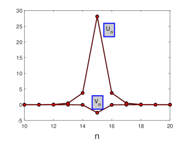
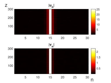
First, in Fig. 1(a) we display an example of a numerically found DES, obtained in the lattice built of $N=100$ sites, and its counterpart. produced by means of the approximation based on Eqs. (9), (10a), (10b), (13), and (12), (16), for values of parameters in Eqs. (1a), (1b) $\epsilon=10$, $q=1$, $\gamma_{1}=\gamma_{2}=-0.05$ (recall that $\gamma_{1,2}<0$ implies the defocusing sign of the $\chi^{(3)}$ nonlinearity) and propagation constant $\omega=0.7$. Because DES is a solution of the codimension-one type, for these arbitrarily chosen parameters the numerical solution can be found only for a specially selected value of the remaining one, viz., the relative strength of the lattice coupling for the SH wave, $\delta\approx 0.9391$, while the analytical approximation yeilds $\delta\approx 0.8645$ [recall that $\delta>0$ implies opposite signs of the SH and FF lattice couplings in Eqs. (1a) and (1b)]. At these values of the parameters, the gap in the linear spectrum of the SH component, as given by Eq. (6), is $0.5<\omega<19.3$, hence $\omega=0.7$ indeed belongs to the band (sitting close to its edge), confirming that the discrete soliton is of the embedded type.

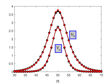
The use of the above approximation, corresponding to the continuum limit, is relevant here, as $\epsilon=10$ is large enough for this purpose. Note also that the relatively small value of the propagation constant, $\omega=0.7$, makes the DES broad enough [as per Eq. (9)], which additionally justifies the use of the quasi-continuum formalism in this case. It is remarkable that the analytical approximation produces a virtually exact DES solution in Fig. 1(a).

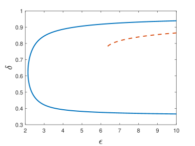
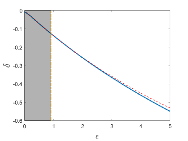
Fixing parameters $q=1$ and $\gamma_{1,2}=-0.05$, and propagation constant $\omega=0.7$ as above, the variation of $\epsilon$ makes it possible to produce two branches of numerical solutions of Eqs. (3a), (3b) in the $\left(\epsilon,\delta\right)$ plane, as shown in Fig. 1(b) by the solid curve with a turning point at $\epsilon=\epsilon_{\min}\approx 2.14$, at which the two branches merge. Thus, Fig. 1(b) shows that the continuation of the DES families does not exist if the coupling constant falls below the minimum value. Note that, for the currently fixed values, $q=1$ and $\omega=0.7$, the SH band, given by Eq. (6), amounts to $\epsilon\delta>0.1$. Obviously, the entire solid curve in Fig. 1(b) belongs to this area. It is also worthy to note that both branches exist at $\delta>\delta_{\min}\approx 0.36$ [in particular, DESs do not exist at $\delta<0$, when the coupling constants in the FF and SH sublattices have the same signs, see Eqs. (1a) and (1b)].

The analytical approximation based on Eqs. (9), (10a), (10b), (13), and (16) produces a single existence branch, shown by the dashed line in Fig. 1(b), which cannot be extended beyond the left end point, i.e., the approximation predicts, in a qualitatively correct form, only one branch of the DES solutions. We assume that this happens because ansatz (9) is not sifficiently versatile to capture the other branch of the solutions. A better ansatz may be tried, but it would lead to an extremely cumbersome analysis.

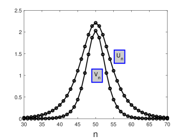
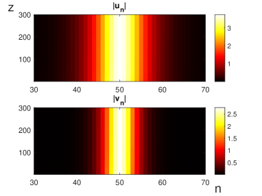
The above results were obtained for a situation close to the continuum limit. Figure 2 presents typical findings for the opposite case, close to the anti-continuum limit, in the lattice composed of $N=30$ sites. First, an example of a strongly discrete embedded soliton is displayed in panel (a) for parameters of Eqs. (1a) and (1b) chosen as $\epsilon=5$, $q=60$, $\gamma_{1}=\gamma_{2}=0.05$, and propagation constant $\omega=29$, while the value of coefficient $\delta$, at which the nongeneric DES is found numerically, is $\delta\approx-0.5496$. Note that the negative sign of $\delta$ implies identical signs of the inter-site coupling in the FF and SH sublattices, on the contrary to the case displayed above in Fig. 1. At these values of the parameters, the SH band, defined by Eq. (7), is $24.5<\omega<30$, to which $\omega=29$ indeed belongs, sitting close to its edge.

The analytical approximation for the strongly discrete DES, based on Eqs. (17), (18), and (23) is also displayed, for the same parameters, in Fig. 2(a). It is seen to be virtually identical to the numerical counterpart.

In a still simpler approximation, which may be applied to a strongly discrete soliton, its FF and SH amplitudes, $U_{0}$ and $V_{0}$, can be found by completely neglecting the coupling of the central site, $n=0$, to the adjacent ones, $n=\pm 1$ [28]. In this limit, Eqs. (3a), (3b) yield, in the expectation of having $U_{0}^{2}\gg V_{0}^{2}$, the following values:

which are close enough to ones observed in Fig. 2(a).

A family of DES modes, produced by the numerical solution of Eqs. (3a), (3b) for the same parameters as in Fig. 2(a), i.e., $q=60$, $\gamma_{1,2}=0.05$, and $\omega=29$, but with a varying coupling constant $\epsilon$, and $\delta$ adjusted accordingly, is displayed in Fig. 2(b), along with its counterpart produced by the above-mentioned analytical approximation, based on Eqs. (17), (18), and (23), It is clearly seen that the approximation is very accurate in this case, even for relatively large values of $\epsilon$, for which the applicability of the anti-continuum formalism is not evident. Unlike the family shown above in Fig. 1, with identical signs of the FF and SH components, the present one always features opposite signs.

Lastly, we note that, for the parameters chosen in Fig. 2(b), Eq. (7) defines the SH band as the area with $|\delta|\epsilon>0.5$. This condition means that the family presented in this figure belongs to the band at $\epsilon>\epsilon_{0}\approx 0.9098$, while its extension to $\epsilon<\epsilon_{0}$ immerses into the bandgap, as a family of regular solitons (non-embedded ones). In the figure, the existence region of the regular solitons is shaded.

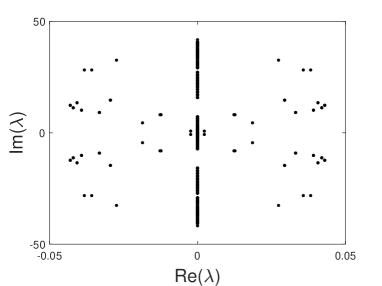
We address the stability of DESs by numerically solving the eigenvalue problem (24a). First, we consider the case of opposite signs of the coupling constant in the SH and FF lattices, i.e., $\delta>0$ in Eq. (1b). The first result is that the solution branches in Fig. 1b are completely unstable. As an illustration, the spectrum of the eigenvalues displayed in Figs. 1a and 1c is shown in Fig. 3. In these cases, the oscillatory instability is accounted for by quartets of complex eigenvalues.

Having established the instability of the DESs shown in Fig. 1a, we display simulations of their dynamics, under the action of two different perturbations, in Fig. 4. First, Fig. 4a demonstrates that the soliton, in spite of the presence of many unstable eigenvalues in its perturbation spectrum, as seen in Fig. 3a, is actually quite robust in direct simulations which include small random perturbations in the initial conditions. In this connection, we note that, with $\epsilon=10$ and $\delta$ close to $1$ (the values used in Fig. 1), and the soliton’s width $W\sim 10$ (as seen in the same figure), the characteristic diffraction (Rayleigh) length is $Z_{\mathrm{diffr}}\sim W^{2}/\epsilon\sim 10$, i.e., the total propagation distance displayed in Fig. 4(a) is $\sim 30$ diffraction lengths, which is actually a very large value in a real experiment [3]-[6]. On the other hand, if the initial state is perturbed merely by multiplying it by factor $0.99$, the DES originally stays nearly intact, over the distance $Z\simeq 60\sim 6Z_{\mathrm{diffr}}$, and then quickly decays, as shown in Fig. 4b. The latter dynamical scenario is typical for the “one-sided” semistability of embedded solitons [9], initiated by slow sub-exponential growth of perturbations, which eventually leads to fast destructiom of the solitons. The perturbed evolution of the DES displayed in Fig. 1c exhibits similar dynamical behavior (not shown here in detail).

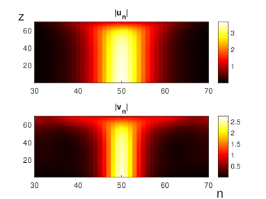
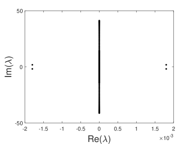
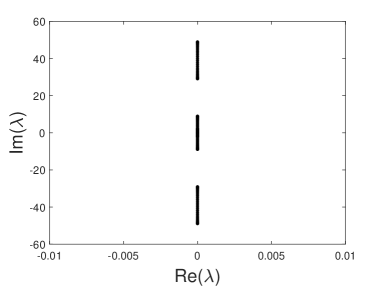
Next, we consider the case of $\delta<0$, i.e., opposite signs of the intersite linear couplings in the FF and SH lattices in Eqs. (1a) and (1b). For the DES shown in Fig. 2a, its linear-perturbation spectrum is plotted in Fig. 5a, which does not include unstable eigenvalues (the spectrum is purely imaginary). This is the case with all DESs along the existence curve plotted in Fig. 2b. Direct simulations of the evolution of the soliton subjected to the scaling perturbation, similar to that which led to the destruction of the semistable soliton in Fig. 4(b), but actually much stronger (with the initial scaling factor $0.9$ instead of $0.99$), demonstrate perfect stability. Under the action of random perturbations, the same soliton is perfectly stable as well (not shown here in detail). Thus, the system of equations (1a) and (1b) with $\delta<0$ produces fully stable DESs, which were not reported before..

References

- [1] Y. R. Shen, The Principles of Nonlinear Optics (Wiley: New York, 1984).
- [2] Y. N. Karamzin and A. P. Sukhorukov, Nonlinear interaction of diffracted light beams in a medium with quadratic nonlinearity – mutual focusing of beams and limitation on efficiency of optical frequency converters, Pisma Zh. Exp. Teor. Fiz. 20, 730 (1974) [JETP Lett. 20, 338 (1975)].
- [3] W. E. Torruellas, Z. Wang, D. J. Hagan, E. W. van Stryland, G. I. Stegeman, L. Torner, and C. R. Menyuk, Observation of 2-dimensional spatial solitary waves in quadratic medium, Phys. Rev. Lett. 74, 5036 (1995).
- [4] G. I. Stegeman, D. J. Hagan, and L. Torner, cascading phenomena and their applications to all-optical signal processing, mode-locking, pulse compression and solitons, Opt. Quantum Electron. 28, 1691-1740 (1996).
- [5] C. Etrich, F. Lederer, B. A. Malomed, T. Peschel, and U. Peschel, Optical solitons in media with a quadratic nonlinearity, Prog. Opt. 41, 483-568 (2000).
- [6] A. V. Buryak, P. Di Tripani, D. V. Skryabin, and S. Trillo, Optical solitons due to quadratic nonlinearities: from basic physics to futuristic applications Phys. Rep. 370, 63-235 (2002).
- [7] M. A. Karpierz, Coupled solitons in waveguides with second- and third-order nonlinearities, Opt. Lett. 20, 1677-1679 (1995).
- [8] A. V. Buryak, Y. S. Kivshar, and S. Trillo, Optical solitons supported by competing nonlinearities, Opt. Lett. 20, 1961-1963 (1995).
- [9] J. Yang, B. A. Malomed, and D. J. Kaup, Embedded solitons in second-harmonic-generating systems, Phys. Rev. Lett. 83, 1958-1961 (1999).
- [10] A. R. Champneys and M. D. Groves, A global investigation of solitary waves solutions to a two-parameter model for water waves, J. Fluid Mech. 342, 199-229 (1997).
- [11] J. Fujioka and A. Espinosa, Soliton-like solution of an extended NLS equation existing in resonance with linear dispersive waves, J. Phys. Soc. Jpn. 66, 2601-2607 (1997).
- [12] A. R. Champneys, B. A. Malomed, J. Yang, and D. J. Kaup. “Embedded solitons”: solitary waves in resonance with the linear spectrum. Physica D 152-153, 340-354 (2001).
- [13] G. Haller, A variational theory of hyperbolic Lagrangian coherent structures, Physica D 240, 574-598 (2011).
- [14] J. K. Yang, Stable embedded solitons, Phys. Rev. Lett. 91, 143903 (2003).
- [15] R. Iwanow, R. Schiek, G. I. Stegeman, T. Pertsch, F. Lederer, Y. Min, and W. Sohler, Observation of discrete quadratic solitons, Phys. Rev. Lett. 93, 113902 (2004).
- [16] F. Lederer, G. I. Stegeman, D. N. Christodoulides, D. N. Christodoulides, G. Assanto, M. Segev, and Y. Silberberg, Discrete solitons in optics, Phys. Rep. 463, 1-126 (2008).
- [17] K. Yagasaki, A. R. Champneys, and B. A. Malomed, Discrete embedded solitons, Nonlinearity 18, 2591-2613 (2005).
- [18] H. S. Eisenberg Y. Silberberg, R. Morandotti, A. Boyd, and J. S. Aitchison, Diffraction management Phys. Rev. Lett. 85, 1863-1866 (2000).
- [19] T. Pertsch, Y. Silberberg, U. Peschel, and F. Lederer, Anomalous refraction and diffraction in discrete optical systems, Phys. Rev. Lett. 88, 093901 (2002).
- [20] D. Cai, A. R. Bishop, and N. Grønbech-Jensen, Localized states in discrete nonlinear Schrödinger equations, Phys. Rev. Lett. 72, 591-595 (1994).
- [21] J. H. Dawes and H. Susanto, Variational approximation and the use of collective coordinates, Phys. Rev. E 87, 063202 (2013).
- [22] B. A. Malomed and M. I. Weinstein, Soliton dynamics in the discrete nonlinear Schrödinger equation, Phys. Lett. A 220, 91-96 (1996).
- [23] D. J. Kaup, Variational solutions for the discrete nonlinear Schrödinger equation, Math. Comp. Simul. 69, 322-333 (2005).
- [24] B. A. Malomed, D. J. Kaup, and R. A. Van Gorder, Unstaggered-staggered solitons in two-component discrete nonlinear Schrödinger lattices, Phys. Rev. E 85, 026604 (2012).
- [25] D. J. Kaup and B. A. Malomed, Embedded solitons in Lagrangian and semi-Lagrangian Systems, Physica D 184, 153-161 (2003).
- [26] M. Syafwan, H. Susanto, S. M. Cox, and B. A. Malomed, Variational approximations for traveling solitons in a discrete nonlinear Schrödinger equation, J. Phys. A: Math. Theor. 45(7), 075207 (2012).
- [27] R. Rusin, R. Kusdiantara, and H. Susanto, Variational approximations using Gaussian ansatz, false instability, and its remedy in nonlinear Schrödinger lattices, J. Phys. A: Math. Theor. 51(47), 475202 (2018).
- [28] S. Aubry, Breathers in nonlinear lattices: Existence, linear stability and quantization, Physica D 103, 201-250 (1997).