Elastic Coupled Co-clustering for Single-Cell Genomic Data
Abstract
The recent advances in single-cell technologies have enabled us to profile genomic features at unprecedented resolution and datasets from multiple domains are available, including datasets that profile different types of genomic features and datasets that profile the same type of genomic features across different species. These datasets typically have different powers in identifying the unknown cell types through clustering, and data integration can potentially lead to a better performance of clustering algorithms. In this work, we formulate the problem in an unsupervised transfer learning framework, which utilizes knowledge learned from auxiliary dataset to improve the clustering performance of target dataset. The degree of shared information among the target and auxiliary datasets can vary, and their distributions can also be different. To address these challenges, we propose an elastic coupled co-clustering based transfer learning algorithm, by elastically propagating clustering knowledge obtained from the auxiliary dataset to the target dataset. Implementation on single-cell genomic datasets shows that our algorithm greatly improves clustering performance over the traditional learning algorithms. The source code and data sets are available at https://github.com/cuhklinlab/elasticC3
Keywords: Co-clustering, Unsupervised transfer learning, Single-cell genomics
1 Introduction
Clustering aims at grouping a set of objects such that objects in the same cluster are more similar to each other compared to those in other clusters. It has wide applications in many areas, including genomics, where single-cell sequencing technologies have recently been developed. For the analysis of single-cell genomic data, most clustering methods are focused on one data type: SIMLR (Wang et al.,, 2017), SC3 (Kiselev et al.,, 2017), DIMM-SC (Sun et al.,, 2017), SAFE-clustering (Yang et al.,, 2018) and SOUP (Zhu et al.,, 2019) are developed for scRNA-seq data, and chromVAR (Schep et al.,, 2017), scABC (Zamanighomi et al.,, 2018), SCALE (Xiong et al.,, 2019) and cisTopic (Gonzalez-Blas et al.,, 2019) are developed for scATAC-seq data. A more comprehensive discussion is presented in Lin et al., (2019). Some methods are developed for the integrative analysis of single-cell genomic data, including Seurat (Butler et al.,, 2018; Stuart et al.,, 2019), MOFA (Argelaguet et al.,, 2018), coupleNMF (Duren et al.,, 2018), scVDMC (Zhang et al.,, 2018), Harmony (Korsunsky et al.,, 2019), scACE(Lin et al.,, 2019) and MOFA+ (Argelaguet et al.,, 2020). David et al., (2020) presented a more comprehensive discussion on integration of single-cell data across samples, experiments, and types of measurement. In real-world applications, for instance, we may better cluster scATAC-seq data by using the knowledge from scRNA-seq data, or better cluster scRNA-seq data from mouse by inference from human data. This raises a critical question on how can we apply knowledge learned from one dataset in one domain to cluster another dataset from a different domain.
In this paper, we focus on the problem of clustering single-cell genomic data across different domains. For example, we may typically have an auxiliary unlabeled dataset A from one domain (say, scRNA-seq data from human), and a target unlabeled dataset T from a different domain (say, scRNA-seq data from mouse). The two datasets follow different distributions. Target data T may consist of a collection of unlabeled data from which it is hard to learn a good feature representation - clustering directly on T may therefore perform poorly. It may be easier to learn a good feature representation from auxiliary data A, which can be due to its larger sample size or less noise than T. Therefore, incorporating the auxiliary data A, we may achieve better clustering on the target data T. This problem falls in the context of transfer learning, which utilizes knowledge obtained from one learning task to improve the performance of another (Caruana,, 1997; Pan and Yang,, 2009), and it can be considered as an instance of unsupervised transfer learning (Teh et al.,, 2006), since all of the data are unlabeled.
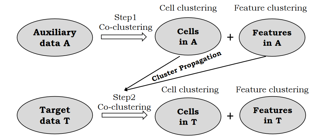
In this work, we propose a novel co-clustering-based transfer learning model to address this problem. A schematic plot of our proposed model is shown in Figure 1. Auxiliary data A and target data T can be regarded as two matrices with cells in the rows and genomic features in the columns. The co-clustering framework (Dhillon et al.,, 2003), which clusters cells and features simultaneously, is utilized in this work. Our proposed approach is composed of two steps: in Step 1, we co-cluster auxiliary data A and obtain the optimal clustering results for cells and features; in Step 2, we co-cluster target data T by transferring knowledge from the clusters of cells and features learned from A. The degree of cluster propagation is elastically controlled by learning adaptively from the data, and we refer to our model as elastic coupled co-clustering (elasticC3). If auxiliary data A and target data T are highly related, the degree of cluster propagation will be higher. On the contrary, if A and T are less related, the degree of knowledge transfer will be lower. The contributions of this paper are as follows:
-
•
To the best of our knowledge, this is the first work introducing unsupervised transfer learning for clustering single-cell genomic data across different data types.
-
•
To ensure wide application, the model proposed in this paper can elastically control the degree of knowledge transfer and is applicable when cluster numbers of cells in auxiliary data and target data are different.
-
•
Our algorithm significantly boosts clustering performance on single-cell genomic data over traditional learning algorithms.
2 Problem Formulation
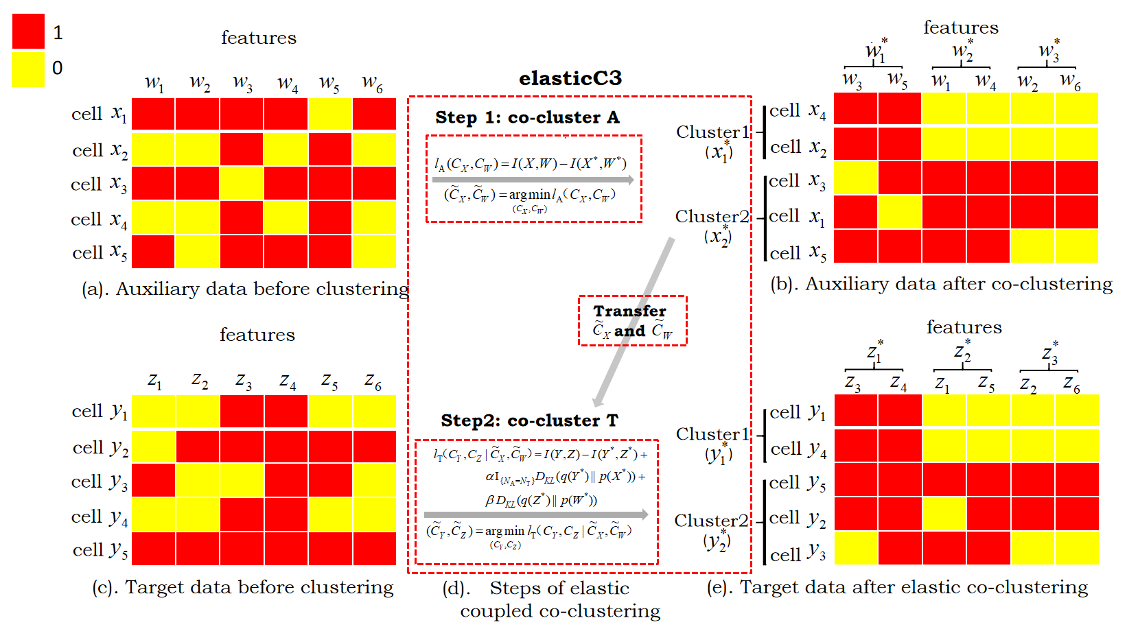
We first use a toy example (Figure 2) to illustrate our method. We regard two matrices as the auxiliary data (denoted as A) and the target data (denoted as T), respectively, with all matrix elements being either 1 or 0. Let and be discrete random variables taking values from the sets of cell indexes in the auxiliary data A and in the target data T, respectively. Let and be discrete random variables for the respective feature spaces of these data, taking values from the sets of feature indexes and . Take the auxiliary data in Figure 2(a) as an example: means the selected cell is the -th cell among the cells and means the selected feature is the -th feature among the features. The meanings of and (Figure 2(c)) are the same as that for and .
Let be the joint probability distribution for and , which can be represented by an matrix. represents the probability of the -th gene being active: the -th gene is expressed in scRNA-seq data or the -th genomic region is accessible in scATAC-seq data in the -th cell. The probability is estimated from the observed auxiliary data A, and we have where the are elements of auxiliary data observations: if the -th feature is active in the -th cell, and otherwise. The marginal probability distributions are then expressed as and . For the target data, is the observed data matrix. is the joint probability distribution for and . and are the marginal probabilities calculated similarly to that in the auxiliary data.
Our goal is to group similar cells and features into clusters (Figure 2(b) and Figure 2(e)). Suppose we want to cluster the cells in auxiliary data A and target data T into and clusters 222Often the number of clusters is unknown, and we usually combine other exploratory analysis including visualization with clustering to determine the number of clusters in practice.correspondingly, and cluster the features in A and T into clusters. Let and be discrete random variables that take values from the sets of cell cluster indexes and , respectively. Let and be discrete random variables that take values from the sets of feature cluster indexes and , respectively. We use and to represent the clustering functions for auxiliary data and indicates that cell belongs to cluster and indicates that feature belongs to cluster . For the target data, the clustering functions and are defined in the same way as that for the auxiliary data. The tuples and are referred to as co-clustering (Dhillon et al.,, 2003).
Let be the joint probability distribution of and , which can be represented as an matrix. This distribution can be expressed as
| (1) |
The marginal probability distributions are then expressed as and . For the target data, , and are defined and calculated similarly to those for the auxiliary data.
The goal of elastic coupled co-clustering in this work is to find the optimal cell clustering function on the target data T by co-clustering the target data and utilizing the information of learned from auxiliary data A (Figure 2(d)).
3 Elastic Coupled Co-clustering Algorithm
In this section, we first present our elastic coupled co-clustering (elasticC3) algorithm, and then discuss its theoretical properties.
3.1 Objective Function
Based on the information theoretic co-clustering (Dhillon et al.,, 2003), the objective function of co-clustering between instances and features is defined as minimizing the loss in mutual information after co-clustering. For auxiliary data A, the objective function of co-clustering can be expressed:
| (2) |
where denotes the mutual information between two random variables:
(Cover and Thomas,, 1991). In practice, we only consider the elements satisfying .
We propose the following objective function for elastic coupled co-clustering of the target data T:
| (3) |
where equals to 1 if and 0 otherwise, , and denotes the Kullback-Leibler divergence between two probability distributions (Cover and Thomas,, 1991), where . The term measures the loss in mutual information after co-clustering for the target data T. and are two distribution-matching terms between A and T after co-clustering, in terms of the row-dimension (cells) and the column-dimension (features), respectively. When the numbers of cell clusters are different between auxiliary data A and target data T (), the distribution-matching term for the row-dimension disappears. and are non-negative hyper-parameters that elastically control how much information should be transferred, and both tend to be higher if the auxiliary data are more similar to the target data. How the parameters and are tuned is discussed in the following section.
3.2 Optimization
The optimization for the objective function in Equation (3) can be divided into two separate steps. In Step 1, as shown at the top of Figure 2(d), we use the co-clustering algorithm by Dhillon et al., (2003) to solve the following optimization problem:
| (4) |
Details are given in A. In Step 2, we transfer the estimated and from Step 1, as shown at the bottom of Figure 2(d), to solve the following optimization problem:
| (5) |
We first rewrite the term in Equation (3) in a similar manner as rewriting in Equations (11), (12) and (13) in A, and we have
| (6) |
where and .
We can iteratively update and to minimize . First, given , minimizing is equivalent to minimizing , where
We iteratively update the cluster assignment for each cell in the target data, fixing the cluster assignment for the other cells:
| (7) |
Second, given , minimizing is equivalent to minimizing
where
We iteratively update the cluster assignment for each feature in the target data, fixing the cluster assignment for the other features:
| (8) |
Summaries of Steps 1 and 2 are given in Algorithm 1. Note that our model has three hyper-parameters: the non-negative and , and K (the number of clusters in feature spaces W and Z). We perform grid-search to choose the optimal combination of parameters, and we will show grid search performs well in both simulated data and real data in Section 4.
3.3 Theoretical Properties
First, we give the monotonically decreasing property of the objective function of the elasticC3 algorithm in the following theorem:
Theorem 1.
Let the value of objective function in the -th iteration be
| (9) |
Then, we have
| (10) |
The proof of Theorem 1 is given in B. Because the search space is finite and the objective function is non-increasing in the iterations, Algorithm 1 converges in a finite number of iterations. Second, our proposed algorithm converges to a local minimum, since finding the global optimal solution is NP-hard.
Finally, we analyze the computational complexity of our algorithm. Suppose the total number of cell-feature co-occurrences (means 1 within data matrices) in the auxiliary dataset is and in the target dataset is . For each iteration, updating and in Step 1 takes , while updating and in Step 2 takes . The number of iterations is in Step 1 and in Step 2. Therefore, the time complexity of our elasticC3 algorithm is . In the experiments, it is shown that is enough for convergence in Figure 3. We may consider the number of clusters , and as constants; thus the time complexity of elasticC3 is . Because our algorithm needs to store all of the cell-feature co-occurrences, it has a space complexity of .
4 Experiments
To evaluate the performance of our algorithm, we conduct experiments on simulated datasets and two single-cell genomic datasets.
4.1 Data Sets
To generate the simulated single-cell data, we follow the simulation setup given in Lin et al., (2019). We set the scATAC-seq data as the auxiliary data A and set the scRNA-seq data as the target data T. We set the number of clusters . Details for generating A and T are given in the C. We set the number of cells in both A and T as , and set the number of features as . We assume that only a subset of features are highly correlated in scRNA-seq and scATAC-seq data, and the other features have no more correlation than random. We vary the percentage of the highly correlated features (percentage = 0.1, 0.5, and 0.9)(details the first column in Table 1).
Our experiment also contains two real single-cell genomic datasets. Real data 1 includes human scRNA-seq data as the auxiliary data and human scATAC-seq data as the target data, where 233 K562 and 91 HL60 scATAC-seq cells are obtained from Buenrostro et al., (2015), and 42 K562 and 54 HL60 deeply sequenced scRNA-seq cells are obtained from Pollen et al., (2014). True cell labels are used as a benchmark for evaluating the performance of the clustering methods. Real data 2 includes human scRNA-seq data as the auxiliary data and mouse scRNA-seq data as the target data. There are three cell types and the datasets are downloaded from panglaodb.se (Fran et al.,, 2019). For the mouse data, 179 pulmonary alveolar type 2 cells, 99 clara cells and 14 ependymal cells are obtained under the accession number SRS4237518. For the human data, 193 pulmonary alveolar type 2 cells, 113 clara cells and 58 ependymal cells are obtained under accession number SRS4660846. We use the cell-type annotation (Angelidis et al.,, 2019) as a benchmark for evaluating the performance of the clustering methods. For each real data, we also consider the setting where by removing one cell type from the auxiliary data, referred as Setting 2 (details in the first column in Table 2).
4.2 Experimental Results
For the simulation analysis, we compare our method with the classic unsupervised transfer clustering method STC (Dai et al.,, 2008) and -means clustering. For real data analysis, we implement variable selection before performing clustering, and select 100 most variable features for each real dataset (D). After variable selection, we binarize the data matrices by setting the non-zero entries to 1. For real data analysis, we compare our method with STC (Dai et al.,, 2008), co-clustering (Dhillon et al.,, 2003) and two commonly used clustering methods for single-cell genomic data, including SC3 (Kiselev et al.,, 2017) and SIMLR (Wang et al.,, 2017). 333For our method elasticC3, we use grid search to tune the hyper-parameters , and K . We choose the search domains , and . The methods STC and co-clustering require input to be binary. Both SC3 and SIMLR use log2(TPM+1) as input for the real scRNA-seq data. The hyper-parameters in STC and co-clustering are also tuned by grid search, as presented in their original publication. Note that the method co-clustering is the same as implementing elasticC3 with and , and no knowledge is transferred between auxiliary data and target data. We use four criteria to evaluate the clustering results, including normalized mutual information (NMI), adjusted Rand index (ARI), Rand index (RI) and purity.
| Simulated Data Setting | Methods | NMI | ARI | RI | purity | |||||
|---|---|---|---|---|---|---|---|---|---|---|
| Setting 1 | elasticC3 | 0.214 | 0.262 | 0.631 | 0.752 | |||||
| STC | 0.142 | 0.172 | 0.586 | 0.701 | ||||||
| -means | 0.116 | 0.136 | 0.568 | 0.671 | ||||||
| Setting 2 | elasticC3 | 0.282 | 0.345 | 0.674 | 0.796 | |||||
| STC | 0.208 | 0.255 | 0.628 | 0.753 | ||||||
| -means | 0.229 | 0.263 | 0.632 | 0.748 | ||||||
| Setting 3 | elasticC3 | 0.379 | 0.454 | 0.727 | 0.837 | |||||
| STC | 0.374 | 0.440 | 0.720 | 0.830 | ||||||
| -means | 0.211 | 0.241 | 0.621 | 0.735 |
| Real Data Sets | Methods | NMI | ARI | RI | purity | |||||
|---|---|---|---|---|---|---|---|---|---|---|
| Real data 1 | elasticC3 (Setting1) | 0.610 | 0.743 | 0.875 | 0.933 | |||||
| A: human scRNA-seq data | elasticC3 (Setting2) | 0.535 | 0.658 | 0.832 | 0.908 | |||||
| T: human scATAC-seq data | STC (Setting1) | 0.495 | 0.616 | 0.811 | 0.895 | |||||
| Setting 1: complete data | STC (Setting2) | 0.472 | 0.587 | 0.796 | 0.885 | |||||
| () | Co-clustering | 0.502 | 0.617 | 0.811 | 0.895 | |||||
| Setting 2: K562 removed from A | SC3 | 0.000 | 0.001 | 0.504 | 0.710 | |||||
| () | SIMLR | 0.025 | 0.046 | 0.525 | 0.710 | |||||
| Real data 2 | elasticC3 (Setting1) | 0.564 | 0.682 | 0.841 | 0.880 | |||||
| A: human scRNA-seq data | elasticC3 (Setting2) | 0.515 | 0.629 | 0.815 | 0.863 | |||||
| T: mouse scRNA-seq data | STC (Setting1) | 0.454 | 0.434 | 0.718 | 0.836 | |||||
| Setting 1: complete data | STC (Setting2) | 0.397 | 0.425 | 0.714 | 0.788 | |||||
| () | Co-clustering | 0.510 | 0.625 | 0.813 | 0.860 | |||||
| Setting 2: alveolar type 2 removed from A | SC3 | 0.378 | 0.318 | 0.661 | 0.849 | |||||
| () | SIMLR | 0.405 | 0.244 | 0.618 | 0.709 |
4.2.1 Performance
We present in Table 1 the clustering results for the simulated scRNA-seq data (target data T). Across different settings, the trends are similar for the four clustering criteria, including NMI, ARI, RI and purity. When the percentage of highly correlated features increases from 0.1 to 0.9, more information is shared among the feature space W for the auxiliary data and the feature space Z for the target data. The clustering results for elasticC3 and STC are improved, because they can transfer more informative knowledge from the auxiliary data to improve clustering of the target data. When the features W and Z are less similar (percentage = 0.1 and 0.5), STC does not perform as well as our method elasticC3, because STC assumes that W and Z are the same, while elasticC3 assumes that W and Z are different and elastically controls the degree of knowledge transfer by introducing the term in Equation (3). When W and Z are more similar (percentage = 0.9), STC is comparable to elasticC3. We also note that our algorithm elasticC3 can adaptively learn the degree of knowledge transferring from the data because the parameters and increase as the similarity of the auxiliary data and target data increases. In Setting 1, the features W and Z are less related and the tuning parameter in elasticC3. Finally, because -means clustering cannot transfer knowledge from auxiliary data to target data, it does not work as well as elasticC3 and STC.
The clustering results for the target data in two real single-cell genomic datasets are shown in Table 2. We see that elasticC3 performs better in Setting 1 than in Setting 2 in the two datasets, because one cell type is removed from the auxiliary data in Setting 2, thereby losing information that can be transferred. Knowledge transfer improves clustering of the target data as elasticC3 outperforms the methods that do not incorporate knowledge transfer, including co-clustering, SC3 and SIMLR in both datasets. The distributions of the features are likely different in the auxiliary data and target data: in real data 1, the distribution of gene expression is likely different from the distribution of promoter accessibility; in real data 2, the distributions of gene expression may be different between human and mouse. STC treats the features in the auxiliary data and target data as the same and performs knowledge transfer. In both datasets, the performance of STC is not as good as that of elasticC3, and it is even worse than that of co-clustering, especially for real data 2. The degree of shared information is likely lower in real data 2, as indicated by the smaller values in and when we implement elasticC3. In summary, elasticC3 adaptively learns the degree of knowledge transfer in auxiliary data and target data, and it outperforms methods that do not allow for knowledge transfer (co-clustering, SC3 and SIMLR) and methods that do not control the degree of knowledge transfer (STC). In addition, elasticC3 works well even when the number of cell clusters differ between auxiliary data and target data, ensuring its wider application.
4.2.2 Convergence
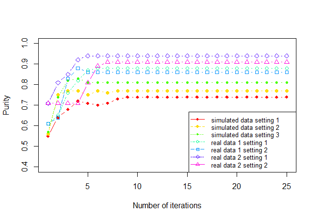
We have proven the convergence of elasticC3 in Theorem 1, and now we show its convergence property empirically. Figure 3 shows the curve of purity vs number of iterations on the seven datasets (For simulated data, we randomly select one run for each setting). Our algorithm elasticC3 converges within 10 iterations. Using the other three clustering criteria gives similar convergence results.
5 Conclusion and Future Work
In this paper, we have developed elasticC3 for the integrative analysis of multiple single-cell genomic datasets. Our proposed method, elasticC3, was developed under the unsupervised transfer learning framework, where the knowledge learned from an auxiliary data is utilized to improve the clustering results of target data. Our algorithm consists of two separate steps. In Step 1, we cluster both the cells and features (i.e. co-cluster) in the auxiliary data, and in Step 2 we co-cluster the target data by elastically transferring the knowledge learned in Step 1. We prove the convergence of elasticC3 to a local optimum. Our algorithm outperforms other commonly used clustering methods in single-cell genomics. Because the framework of elasticC3 is general, we plan to explore its application to other areas, including text mining.
Broader Impact
This work does not present any foreseeable societal consequences and ethical issues.
Acknowledgement
This work has been supported by the Chinese University of Hong Kong direct grant 2018/2019 No. 4053360, the Chinese University of Hong Kong startup grant No. 4930181, and Hong Kong Research Grant Council Grant ECS No. CUHK 24301419.
References
- Angelidis et al., (2019) Angelidis, I., Simon, L. M., Fernandez, I. E., Strunz, M., and Mayr, C. H. (2019). An atlas of the aging lung mapped by single cell transcriptomics and deep tissue proteomics. Nat. Commun, 10(963).
- Argelaguet et al., (2020) Argelaguet, R., Arnol, D., Bredikhin, D., and so on (2020). Mofa+: a statistical framework for comprehensive integration of multi-modal single-cell data. Genome Biol, 21(111).
- Argelaguet et al., (2018) Argelaguet, R., Velten, B., Arnol, D., Dietrich, S., Marioni, J. C., and so on (2018). Multi-omics factor analysis-a framework for unsupervised integration of multi-omics data sets. Mol Syst Biol, 14.
- Buenrostro et al., (2015) Buenrostro, J. D., Wu, B., Litzenburger, U. M., Ruff, D., Gonzales, M. L., Snyder, M. P., Chang, H. Y., and Greenleaf, W. J. (2015). Single-cell chromatin accessibility reveals principles of regulatory variation. Nature, (523):486–490.
- Butler et al., (2018) Butler, A., Hoffman, P., Smibert, P., Papalexi, E., and Satija, R. (2018). Integrating single-cell transcriptomic data across different conditions, technologies and species. Nat. Biotechnol., 36:411–420.
- Caruana, (1997) Caruana, R. (1997). Multitask learning. Machine Learning, 28:41–75.
- Cover and Thomas, (1991) Cover, T. M. and Thomas, J. A. (1991). Elements of information theory. Wiley-Interscience.
- Dai et al., (2008) Dai, W. Y., Yang, Q., Xue, G. R., and Yu, Y. (2008). Self-taught clustering. Proceedings of the 25th international Conference on Machine Learning.
- David et al., (2020) David, L., Johannes, K., Ewa, S., and so on (2020). Eleven grand challenges in single-cell data science. Genome Biol, 21(31).
- Dhillon et al., (2003) Dhillon, I. S., Mallela, S., and Modha, D. S. (2003). Information-theoretic co-clustering. Proceedings of the Ninth ACM SIGKDD International Conference on Knowledge Discovery and Data Mining, pages 89–98.
- Duren et al., (2018) Duren, Z., Chen, X., Zamanighomi, M., Zeng, W., Satpathy, A., Chang, H., Wang, Y., and Wong, W. H. (2018). Integrative analysis of single cell genomics data by coupled non-negative matrix factorizations. Proc. Natl. Acad. Sci., (115):7723–7728.
- Fran et al., (2019) Fran, O., Gan, G. M., and Johan, L. M. B. (2019). Panglaodb:a web serer for exploration of mouse and human single-cell rna sequencing data. Database.
- Gonzalez-Blas et al., (2019) Gonzalez-Blas, C. B. et al. (2019). cistopic: cis-regulatory topic modeling on single-cell atac-seq data. Nat. Methods, 16:397–400.
- Kiselev et al., (2017) Kiselev, V. Y., Kirschner, K., Schaub, M. T., Andrews, T., Yiu, A., Chandra, T., Natarajan, K. N., Reik, W., Barahona, M., et al. (2017). Sc3: Consensus clustering of single-cell rna-seq data. Nat. Methods, 14(483).
- Korsunsky et al., (2019) Korsunsky, I., Millard, N., Fan, J., Slowikowski, K., Zhang, F., and so on (2019). Fast, sensitive and accurate integration of single-cell data with harmony. Nat.Methods., 16(12):1289–1296.
- Lin et al., (2019) Lin, Z. X., Zamanighomi, M., Daley, T., Ma, S., and Wong, W. H. (2019). Model-based approach to the joint analysis of single-cell data on chromatin accessibility and gene expression. Stat. Sci.
- Love et al., (2014) Love, M. I., Huber, W., and Anders, S. (2014). Moderated estimation of fold change and dispersion for rna-seq data with deseq2. Genome Biol, 15(550).
- Pan and Yang, (2009) Pan, S. J. and Yang, Q. (2009). A survey on transfer learning.
- Pollen et al., (2014) Pollen, A. A., Nowakowski, T. J., Shuga, J., Wang, X., and Leyrat, A. A. (2014). Low-coverage single-cell mrna sequencing reveals cellular heterogeneity and activated signaling pathways in developing cerebral cortex. Nat. Biotechnol, (32):1053–1058.
- Schep et al., (2017) Schep, N. A., Wu, B., Buenrostro, J. D., and Greenleaf, W. J. (2017). chromvar: inferring transcription-factor-associated accessibility from single-cell epigenomic data. Nat. Methods, 14:975–978.
- Stuart et al., (2019) Stuart, T., Butler, A., Hoffman, P., and so on (2019). Comprehensive integration of single-cell data. Cell, 177(7):1888–1902.
- Sun et al., (2017) Sun, Z., Wang, T., Deng, K., Wang, X. F., Lafyatis, R., Ding, Y., Hu, M., and Chen, W. (2017). Dimm-sc: A dirichlet mixture model for clustering droplet-based single cell transcriptomic data. Bioinformatics, (34):139–146.
- Teh et al., (2006) Teh, Y. W., Jordan, M. I., Beal, M. J., and Blei, D. M. (2006). Hierarchical dirichlet processes. J. Am. Stat. Assoc, (101):1566–1581.
- Wang et al., (2017) Wang, B., Zhu, J., Pierson, E., Ramazzotti, D., and Batzoglou, S. (2017). Visualization and analysis of single-cell rna-seq data by kernel-based similarity learning. Nat. Methods, 14:414–416.
- Xiong et al., (2019) Xiong, L., Xu, K., Tian, K., Shao, Y., Tang, L., Gao, G., Zhang, M., Jiang, T., and Zhang, Q. C. (2019). Scale method for single-cell atac-seq analysis via latent feature extraction. Nat. Commun, 10(4576).
- Yang et al., (2018) Yang, Y., Huh, R., Culpepper, H. W., Lin, Y., Love, M. I., and Li, Y. (2018). Safe-clustering: Single-cell aggregated(from ensemble)clustering for single-cell rna-seq data. Bioinformatics.
- Zamanighomi et al., (2018) Zamanighomi, M., Lin, Z., Daley, T., Chen, X., Duren, Z., Schep, A., Greenleaf, W. J., and Wong, W. H. (2018). Unsupervised clustering and epigenetic classification of single cells. Nat. Commun, 9(2410).
- Zhang et al., (2018) Zhang, H., Lee, C. A. A., Li, Z., and the others (2018). A multitask clustering approach for single-cell rna-seq analysis in recessive dystrophic epidermolysis bullosa. PLoS Comput Biol, 14(4).
- Zhu et al., (2019) Zhu, L., Lei, J., Klei, L., Devlin, B., and Roeder, K. (2019). Semisoft clustering of single-cell data. Proc. Natl. Acad. Sci. USA, 116:466–471.
Appendix A Details of Step 1 in elasticC3 algorithm
The optimization problem
is non-convex and challenging to solve. We rewrite this objective function in the form of KL divergence, since the reformulated objective function is easier to optimize. To be more specific,
| (11) |
where is expressed as
| (12) |
The distributions , , , , are estimated as in Section 2 in the text. Further, we have
| (13) |
where and . The relations in Equations (11) and (13) have been proven by Dhillon et al., (2003) and Dai et al., (2008).
To minimize , we can iteratively update and as follows.
-
•
Fix and iteratively update the cluster assignment for each cell in the auxiliary data, while fixing the cluster assignments for the other cells:
(14) -
•
Fix and iteratively update the cluster assignment for each feature in the auxiliary data, while fixing the cluster assignments for the other features:
(15)
Appendix B Proof of Theorem 1
Appendix C Steps of data generation in simulation study
Similar to the simulation scheme in Lin et al., (2019), we generate data in simulation study as in the following:
-
1.
Generate and .
. ;.
-
2.
Generate and . The cluster labels are generated with equal probability 0.5.
-
3.
Generate and . if , where if ; otherwise.
-
4.
Generate and . if , where if ; otherwise; .
-
5.
Generate and . if and if ; if and if .
-
6.
Generate target data T and auxiliary data A. if and otherwise; if and otherwise.
More details on the notations and the simulation scheme is presented in Lin et al., (2019). In our simulation, the difference on the steps of data generation from that in Lin et al., (2019) is the addition of Step 6, which generates binary data. means gene is expressed in cell , and otherwise. means the promoter region for feature is accessible in cell , and otherwise.
Appendix D Details of feature selection for real data
In the experiment, we implement variable selection for real single-cell genomic datasets before performing clustering, for the purpose of speeding up computation and balances the number of variables among different data types. For real data 1, we apply clustering to the individual datasets (Zamanighomi et al.,, 2018) and then select cluster-specific features (Love et al.,, 2014; Zamanighomi et al.,, 2018). Using the R toolkit Seurat (Butler et al.,, 2018; Stuart et al.,, 2019), we select 100 most variable cluster-specific genes in each of scATAC-seq and scRNA-seq data. For real data 2, we also use Seurat to select the 100 most variable homologs from each of the mouse and human scRNA-seq data.