Einstein metrics of cohomogeneity one with as principal orbit
Abstract
In this article, we construct non-compact complete Einstein metrics on two infinite series of manifolds. The first series of manifolds are vector bundles with as principal orbit and as singular orbit. The second series of manifolds are with the same principal orbit. For each case, a continuous 1-parameter family of complete Ricci-flat metrics and a continuous 2-parameter family of complete negative Einstein metrics are constructed. In particular, metrics and discovered by Cvetič et al. in 2004 are recovered in the Ricci-flat family. A Ricci flat metric with conical singularity is also constructed on . Asymptotic limits of all Einstein metrics constructed are studied. Most of the Ricci-flat metrics are asymptotically locally conical (ALC). Asymptotically conical (AC) metrics are found on the boundary of the Ricci-flat family. All the negative Einstein metrics constructed are asymptotically hyperbolic (AH).
1 Introduction
A Riemannian manifold is Einstein if its Ricci curvature satisfies for some constant . A Riemannian manifold is of cohomogeneity one if a Lie Group acts isometrically on with principal orbit of codimension one. The Einstein equations of a cohomogeneity one manifold is reduced to a dynamic system.
In this article we focus on constructing non-compact cohomogeneity one Einstein metrics. Known examples include the first inhomogeneous Einstein metric in [Cal75], which has Kähler holonomy. More non-compact Kähler–Einstein metrics of cohomogeneity one were constructed in [BB82][DW98][WW98][DS02]. Non-compact cohomogeneity one and metrics, which are motivations to this article, were constructed in [BS89][GPP90][CGLP04][FHN18]. Fixing the principal orbit , we aim to look into the full dynamic system of cohomogeneity one Einstein metrics without imposing any special holonomy condition. Odd dimensional cohomogeneity one Einstein metrics with generic holonomy include those constructed in [BB82][WW98][Che11]. The case where the isotropy representation of the principal orbit consists of exactly two inequivalent irreducible summands was studied in [Böh99][Win17]. Examples where the principal orbit is a product of irreducible homogeneous spaces was constructed in [Böh99]. In [Chi19b], Ricci-flat metrics with Wallach spaces as principal orbits were constructed. The isotropy representation of Wallach spaces consists of three inequivalent irreducible summands, two of which are from the singular orbit, allowing the singular orbit to be squashed. In this article, the principal orbit also consists of three irreducible summands. Our main results are the following.
Theorem 1.1.
Let be the -bundle over given by the group triple . There exists a continuous -parameter family of smooth Einstein metrics of cohomogeneity one on . Specifically,
-
1.
is a continuous 1-parameter family of complete Ricci-flat metrics on . A metric in this family is AC if , it is ALC otherwise. For , each has holonomy on . For , each with has generic holonomy.
-
2.
with is a continuous 2-parameter family of complete AH negative Einstein metrics on .
Some known Einstein metrics are recovered in this family. In the case where , is the metric in [BS89][GPP90]. The 1-parameter family of metrics was constructed in [CGLP04]. For all , metrics are of two summands type. They were constructed in [Böh99][Win17]. All the other metrics in are new to the author.
On , we have the following.
Theorem 1.2.
There exists a continuous -parameter family of smooth Einstein metrics of cohomogeneity one on . Specifically,
-
1.
is a continuous 1-parameter family of complete Ricci-flat metric on . A metric in this family is AC if , it is ALC otherwise. For , is on and all the other Ricci-flat metrics have generic holonomy. For , each with has generic holonomy.
-
2.
with is a continuous 2-parameter family of complete AH negative Einstein metric on . In particular, is the hyperbolic cone with base the standard .
Although not included in the theorem above, the parameter can be the origin for . The metric represented is the Euclidean metric on , as shown in Section 3. Metrics are of two summand type. They first appeared in [BB82]. Metrics is also of two summands type. They were constructed in [Chi19a]. In the case where , is the metric with the opposite chirality to the metric constructed in [CGLP04]. All the other metrics in are new to the author.
In some sense, the 2-dimensional parameter in Theorem 1.1 and Theorem 1.2 controls the asymptotic limit of the metric represented. The non-vanishing of in gives the ALC asymptotics. The parameter also describes how the principal orbit is squashed near the singular orbit. More details are discussed in Section 3. The non-vanishing of gives the AH asymptotics. As discussed in Section 2, the dynamic system of the negative Einstein metrics has a subsystem that can represent the Ricci-flat system. Integral curves with are solutions of this subsystem.
New Taub-NUT metrics on with conical singularity at the origin are also constructed.
Theorem 1.3.
There exists a continuous -parameter family of Einstein metrics of cohomogeneity one on . They all have conical singularity at the origin. Specifically,
-
1.
a singular ALC Ricci-flat metric on . For , the metric is on . For , the metric has generic holonomy.
-
2.
with is a continuous 1-parameter family of singular AH negative Einstein metric on .
Consider the holonomy of the Ricci-flat metrics in Theorems 1.1-1.3. Combining our Lemma 6.5 with Theorem 2.1 in [Hit74] and [Wan89], we obtain the following.
Theorem 1.4.
In particular for , the continuous family of Ricci-flat metrics has the metric lies in the interior and all the other Ricci-flat metrics have generic holonomy. Hence the parallel spinor on is not preserved under a continuous deformation of Ricci-flat metrics through the family . Such a phenomenon also occurs for holonomy [Chi19b]. Parallel spinors are preserved under a continuous deformation of Ricci-flat metrics if the manifold is compact. Please see Theorem A in [Wan91] for more details.
Principal orbit of manifolds studied in this article are from the group triple given by
The principal orbit is the total space of quaternionic Hopf fibration
| (1.1) |
Take as the space of unit quaternionic vector in . The fibration is given by . The transitive action of on is given by
| (1.2) |
for each . The isotropy group for is . The action of passes down to the base. The isotropy group for is . Therefore, the quaternionic Hopf fibration is indeed the homogeneous fibration More details of the isotropy representation are discussed in the next section.
Let be the cohomogeneity one manifold with principal orbit and singular orbit . Then is an bundle over . A cohomogeneity one metric on has the form of , where is an invariant metric on each with and it collapse to an invariant metric on as . We also construct cohomogeneity one Einstein manifolds where the singular orbit for these manifolds is a singleton. In that scenario, the homogeneous part vanishes as . Since the principal orbit is , the cohomogeneity one manifold is topologically .
One feature of the case in this article that differs from the one in [Chi19b] is that the singular orbit is irreducible and the fiber is of two irreducible summands. Moreover, irreducible summands in all have different dimensions, as shown in Section 2. The cohomogeneity one dynamic systems have less symmetry than the one in [Chi19b]. It is worth mentioning that the cohomogeneity one equation in the article shares some degree of similarity with the one that appears in [Rei11]. The study may help shed some light on the global existence question of metric with an Aloff–Wallach space as the principal orbit.
Remark 1.5.
There exists an intermediate group between and . With the same group action (1.2) of , we can see that the group triple gives the complex Hopf fibration
| (1.3) |
Let be the vector bundle with principal orbit and singular orbit . It is a natural question to ask if there are more complete cohomogeneity one Einstein metrics on besides those constructed in [BB82]. Specifically, isotropy representation of has two irreducible summands that allow each with to be squashed and is a -invariant metric on a circle bundle over a squashed .
The Einstein metrics constructed and recovered in this article have three kinds of asymptotic behaviors. We give definitions in the following.
Definition 1.6.
Let be a Riemannian manifold of dimension . Let be an -dimensional Riemannian manifolds and be the metric cone with base . Let denote the tip of the cone. is asymptotically conical (AC) if for some , we have in the pointed Gromov–Hausdorff sense.
Remark 1.7.
Note that if in Definition 1.6 is a standard sphere , the metric is the Euclidean metric on . Then is asymptotically Euclidean (AE).
Definition 1.8.
Let be a Riemannian manifold of dimension . Let be an -dimensional Riemannian manifolds and be the metric cone with base . is asymptotically locally conical (ALC) if for some , we have in the pointed Gromov–Hausdorff sense, where is some -bundle over and is a constant.
Definition 1.9.
Let be a Riemannian manifolds of dimension with a boundary . is conformally compact if there exists a positive function such that extends to a smooth metric on .
In Definition 1.9, it can be checked that sectional curvature of approaches to near . If is negative Einstein, then the sectional curvature must approach to a constant near . With normalization, we fix . Hence a conformally compact Einstein manifold is also called an asymptotically hyperbolic (AH) manifold.
This article is structured as the following. In Section 2, we derive the cohomogeneity one Einstein equation with principal orbit . Then finding a cohomogeneity one Einstein metric is equivalent to finding an integral curve defined on . Then we apply coordinate change inspired by the one in [DW09a][DW09b]. In the new coordinate, initial conditions and the asymptotic limits of the original system are transformed to critical points. Then the construction of Einstein metrics boils down to finding integral curves that emanate from one critical point and tend to the other. Proving the completeness of the metric is equivalent to showing that the new integral curve is defined on .
In Section 3, we compute linearizations of some critical points with geometric significance of the new system. There are three critical points that represents different initial conditions. One of them gives the smooth extension of the metric to ; one gives the smooth extension of the metric to the origin of ; and third one gives the singular extension to the origin of . There are two types of critical points that represent different asymptotic limits. One of them represents the ALC limit and the other type serves as the AH limit for the integral curves.
In Section 4, we construct a compact invariant set that contains sellected critical points in the previous section on its boundary. Linearization in the previous section helps to prove that some integral curves that emanate from these points are in the compact invariant set initially. Hence the completeness of the represented metrics follows. The technique we use is very similar to the one in [Chi19a].
2 Einstein Equation
We derive the Einstein equation in this section. We first introduce some notation regarding representation theory. Let be the trivial representation. Let be the matrix multiplication representation (over complex numbers) of . Let denote the -th symmetric tensor power of the matrix multiplication representation (over complex numbers) of (hence ). Let denote the complex representation of of weight . Define the inner product for as . Note that is non-degenerate on and equal to a multiple of the Killing form of when restricted to .
The action of on is equivalent to the adjoint action of on . Let . We have the following -orthogonal decomposition for .
| (2.1) |
Consider and embed in . Identify with . The isotropy representation of hence has a -orthonormal basis , where
| (2.2) |
and each is given by
with
The trivial representation is spanned by , which is orthogonal to . Note that , where and are respectively the Killing form for and . We abuse the notation by using to denote the invariant metric on that is induced by the inner product. Take as the background metric. By Schur’s Lemma, an invariant metric on has the form of
| (2.3) |
By Corollary 7.39 in [Bes08], the formula of the scalar curvature for is
Compute the first variation of the Hilbert–Einstein functional on . The Ricci endomorphism is given by
| (2.4) |
Note that and are both -diffeomorphic to . We construct Einstein metrics by setting as a geodesic and assign -invariant metric on each . Then (2.3) becomes a -valued function on , where is the space of -invariant symmetric 2-tensor. By [EW00], the cohomogeneity one Einstein system is
| (2.5) |
with conservation law
| (2.6) |
There are three possible initial conditions for (2.5). The first possibility is having as the singular orbit. The cohomogeneity one manifold is an -bundle over . The principal orbit becomes the zero section as . In order to smoothly extend the metric on the tubular neighbourhood around , we have the following proposition.
Proposition 2.1.
The necessary and sufficient conditions for the metric to extend smoothly to a metric in a tubular neighborhood of is
| (2.7) |
for some .
Proof.
Since the unit sphere in is generated by , and . It is clear that is the standard metric for . The initial condition is then derived by Lemma 9.114 in [Bes08]. ∎
Another possible initial condition is collapsing to a singleton as . Since , the cohomogeneity one manifold is topologically . In order to extend the metric on the neighborhood of the origin of , we have the following proposition.
Proposition 2.2.
The necessary and sufficient conditions for the metric to extend smoothly to a metric in a tubular neighborhood of origin in is
| (2.8) |
Proof.
The unit sphere is generated by and ’s. Therefore, if
is the flat metric on . The initial condition is obtained by Lemma 9.114 in [Bes08]. ∎
Note that admits two homogeneous Einstein metrics. Hence for a cohomogeneity one metric of Taub-NUT type, can also degenerate to a point as a Jensen sphere [Jen73]. Then the corresponding initial condition is given by
| (2.9) |
where . In other words, if
then is a singular cone metric on with the Jensen sphere as its base.
As pointed out in Remark 2.9 in [Chi19b], in the Ricci-flat case, changing in (2.7) is essentially the homothetic change of the solution around . Moreover, (2.7) does not fully determine the metric in a tubular neighborhood of . This is also the case for (2.8). Using Lemma 1.1 in [EW00], we can prove that there exists a free parameter for of order 3 for (2.7) and (2.8). We consider (2.7) bellow. Statements concerning (2.8) can be obtained without substantial change of the argument.
We first rephrase Lemma 1.1 in [EW00] for below.
Lemma 2.3 ([EW00]).
Let be the slice representation for . Let be the space of -equivariant homogeneous polynomials of degree . Consider a smooth curve with Taylor expansion around . The curve can be smoothly extended to as a symmetric 2-tensor if and only if each is an evaluation of some element in at .
Since and are inequivalent, we have decomposition
By induction, we have
| (2.10) |
as -modules. In particular, we have
We also have
| (2.11) |
where . Hence it is clear that
Proposition 2.4.
For initial condition (2.7), there exists a free parameter for of order 3.
Proof.
Identify as a map , where and . In that way, the standard inner product on each fiber is given by .
The Taylor expansion can be written as
| (2.12) |
Since for and is spanned by the identity matrix, we learn that is determined by . Hence no free variable of higher order comes from the component.
The generator for is the identity matrix . Hence one of the generators of is . Note that the identity map in is clearly -equivariant. Hence the matrix , where is another generator of . By straightforward computation, the third generator of is the projection map from to the 3-dimensional subspace of .
Evaluate these three generators at and take into account that is a unit speed geodesic. We learn that and is a multiple of
for some . Since , there are in principle two free variables for to extend smoothly around as a 2-tensor. However, with the geometric setting that is a unit geodesic, the parameter is determined. Therefore, can be extended smoothly around if
| (2.13) |
where for some . ∎
Remark 2.5.
Proposition 2.4 can be carried over to (2.8) by thinking as a vector bundle over a singleton. In this case, is the isotropy representation at . The space to consider is , where is the slice representation by the action of . Lemma 2.3 can then be applied with no extra difficulties. Besides the discussion above, there is an alternative procedure to derive the smoothness condition. More details are presented in [VZ20].
Inspired by [DW09a][DW09b], we apply coordinate change . The quantity is the trace of the shape operator of the hypersurface orbit. Define
| (2.14) |
Define functions on
| (2.15) |
Let ′ denote the derivative with respect to . The Einstein equations (2.5) become a polynomial system
| (2.16) |
with conservation law (2.6) becomes
| (2.17) |
It is clear that from the definition of coordinate change. In fact, let
one can check that is a flow-invariant -dimensional manifold in with a -dimensional boundary .
Remark 2.6.
For (2.16) with , the variable and functions , and are recovered by
| (2.18) |
Remark 2.7.
If we assume in (2.20). Since in this case, we have
Since , the variable and functions , and can be recovered without . Therefore, for cohomogeneity one Ricci-flat metrics, we consider the vector field on the 4-dimensional invariant manifold
given by with all terms deleted.
On the other hand, it is clear (2.16) has a subsystem restricted on . Consider the map by . It is clear that and are -related. Therefore, cohomogeneity one Ricci-flat metrics can be represented by integral curves on , even though the quantity does not actually vanish on the Ricci-flat manifold.
Remark 2.8.
Note that (2.5) is not invariant under homothety change if . We fix in this article to fix the homothety for negative Einstein metrics.
If in (2.5), then the original system is invariant under homothety change. The homothety change is transformed to the shifting of for an integral curve, while the graph of the integral curve remains unchanged. Combining with Remark 2.7, we know that each integral curve for restricted on represents a solution in the original coordinate up to homothety.
For a technical reason that is further discussed in Remark 3.1 in Section 3, instead of studying system (2.16) on , we study a dynamic system that is equivalent to (2.16). Remark 2.6, Remark 2.7 and Remark 2.8 are carried over.
On , define
It is a -dimensional surface in with a boundary. Define
| (2.19) |
by sending to . It is straightforward to check that is a diffeomorphism. On , define function . Consider the dynamic system
| (2.20) |
on . By straightforward computation, we have
| (2.21) |
from which we deduce
Therefore, the boundary
is flow-invariant. Moreover, and are -related. We have the following commutative diagram.
| (2.22) |
The variable and functions , and can be recovered by replacing with in Remark 2.6 and Remark 2.7. By Remark 2.7 and Remark 2.8, we fix in in order to fix the homothety for negative Einstein metrics. Each integral curve for restricted on represents a Ricci-flat solution in the original coordinate up to homothety. Define . It is clear that is flow-invariant. By the discussion above, it is justified to denote as .
Proposition 2.9.
Proof.
The Ricci-flat case was proven in Lemma 5.1 [BDW15]. As for the negative Einstein case, since along the corresponding integral curve, it is clear that is increasing along the curve. Hence we have . The proof is complete. ∎
To some extent, by the proposition above, the problem of constructing a cohomogeneity one Einstein metric on is transformed to finding an integral curve of (2.20) on that is defined on . The initial conditions at are transformed to limits of these integral curves as . In Section 3, we see that initial conditions (2.7), (2.8) and (2.9) are transformed to critical points of the new system. Hence the next step is to show that integral curves that emanate from theses critical points are defined on .
There are some integral curves already known to be defined on . These curves lie in several subsystems of (2.20) besides . We give a short summary in the following.
Straightforward computation shows that
is flow-invariant. Integral curves on this set represents metrics with imposed. Hence the 3-sphere is round (hence the subscript “Rd”) and the subsystem is of two summands type. This case is studied in [Win17][Böh99]. Furthermore, for , there exists an integral curve that represents the metric in [BS89][GPP90]. The metric can be represented by a straight line in terms of variables in (2.14).
One can also see that
is flow-invariant. Integral curves on this set represents cohomogeneity one metrics with imposed. Under this setting, the homogeneous metric on is the Fubini–Study metric and it is Kähler–Einstein. The imposed equation is also part of the Kähler condition shown in [DW98]. The circle bundle over is classified by the multiple of an indivisible integral cohomology class in . For our case in , the principal orbit is the circle bundle over the Kähler–Einstein . This case is included in [BB82].
The reduced system on the invariant set
carries two pieces of information. On one hand, if while at the infinity of some cohomogeneity one Einstein metrics, variables and converge to zero along the corresponding integral curve. Hence serves as the “invariant set of ALC limit”. On the other hand, the subsystem on is essentially the one that appears in [Win17][Böh99] with respect to the group triple . For , there exists a metric on the cohomogeneity one space [BS89][GPP90]. The metric can be represented by a straight line in terms of variables in (2.14).
Finally, for , there exists a pair of invariant sets that represent the conditions of positive/negative chirality. This case is studied in [CGLP04] and a continuous 1-parameter family of metrics is discovered. On one boundary of this family lies the metric in [BS89][GPP90]. This case is discussed in more details in Section 6.3.
3 Critical Points
We study critical points of vector field in (2.20) in this section. Let be a critical point of . If an integral curve defined on has as its limit as , then the coordinates of represent the initial condition for the metric as up to the first order. Indeed, we see that initial conditions (2.7), (2.8) and (2.9) are transformed to critical points. On the other hand, if the integral curve has as its limit as , then represents the asymptotic limit for the metric as up to first order. A critical point can carry these two pieces of information simultaneously.
Through computing linearizations at these points, we are able to prove the existence of Einstein metrics that are defined on a tubular neighbourhood around and a neighbourhood around the origin of . The proof for the completeness of these metrics then boils down to showing that these integral curves are defined on .
On , where the function vanishes, we have the following critical points and boundary conditions.
-
1.
-
2.
-
(a)
-
(b)
-
(a)
-
3.
-
(a)
-
(b)
-
(a)
-
4.
-
5.
-
6.
-
7.
On , we have the following.
-
1.
-
2.
-
3.
In this article, we mainly focus on critical points , , , and . With the help of the software Maple, we compute the linearization of (2.20) at these critical points and compute the eigenvalues and eigenvectors. As we only consider system (2.20) restricted on . We only focus on eigenvectors that are tangent to , i.e., orthogonal to the normal vector field on . Note that is the intersection of and the algebraic surface . Therefore, for integral curves that stay in , eigenvectors are orthogonal to the normal vector field on the algebraic surface in addition to . We have
3.1
For an integral curve that emanates from , one can show that the point is (2.7) under the new coordinate (2.20). Integral curves emanating from this point represent smooth Einstein metrics on the tubular neighbourhood of . The linearization at the point is
| (3.1) |
Eigenvalues, along with their respective eigenvectors that are tangent to , are the following.
| (3.2) |
Hence the general linearized solution emanating from is of the form
| (3.3) |
for some constants . Note that the correspondence between germs of linearized solution (3.3) and is not 1 to 1. For example, and give the same linearized solution. The redundancy is cut out by fixing . By Hartman–Grobman theorem, there is a 1 to 1 correspondence between each choice of and an actual solution curve that emanates . Hence we can use to denote the actual solution that approaches to (3.3) near . Moreover, by the unstable version of Theorem 4.5 in [CL55], there is some that
| (3.4) |
Remark 3.1.
Here we explain the advantage of using system (2.20) instead of (2.16). The linearization of (2.16) at has two distinct positive eigenvalues. Hence the error term of a linearized solution may dominates terms with the smaller eigenvalues, which create extra difficulties in estimating a function near . In (3.4), we only have one positive eigenvalue. As the error of the linearized solution is dominated near , we can safely make an estimate using the linearized solution.
In this article, we consider with and . In order the let enter initially, we must have so that is positive initially along the curve. The geometric meaning of having is to allow to be squashed in a way that for . Whether there exists a complete metric that is represented by with is to be known. In order to let enter initially, we must have .
It is clear that . Since is parallel to
one can check that and are orthogonal to . Therefore, the 1-parameter family stays in the invariant set . Hence each near in represents a Ricci-flat metric defined on the tubular neighborhood around . Each with near represents a negative Einstein metric defined on the tubular neighborhood around .
There are some known to be defined on . Note that lies on . These integral curves are of two summands type. By [Win17][Böh99], we know that each is an integral curve on that originates from and tends to and each with is an integral curves that originates from and tend to . with in the case were studied in [CGLP04]. These integral curves all tend to . In Section 4, we construct a compact invariant set that contains all with .
3.2 and
Consider It is clear that the point corresponds to the initial condition (2.8). We have
| (3.5) |
Eigenvectors, along with their respective eigenvalues, that are tangent to are the following.
| (3.6) |
Therefore, there exists a 2-parameter family of integral curves with that emanate from such that
| (3.7) |
In this article, we consider with . The choice for is to allow the in to be squashed in a way that for . The geometric meaning of having is the same as the one for . In order the let enter initially, we must have .
One can check that . Since is parallel to
it is clear that is a 1-parameter family of integral curves that stay in . Hence one obtain a 1-parameter family of Ricci-flat metrics and a 2-parameter family of negative Einstein metrics on the neighborhood around the origin in .
Some are known to be defined on . A trivial example is that represent the standard Euclidean metric. With and , stays in , with and for [Chi19a]. Moreover, is simply the hyperbolic cone with the standard sphere as its base. It is also known that stays in . In particular, is the almost Kähler–Einstein metric with as its limit [BB82][Bes08, Theorem 9.130]. For , we know that for some . As shown in Section 6.2, there also exists an isolated example for another value of , which is the quaternionic Kähler metric constructed in [Swa91].
As for , where and , the point corresponds to initial condition (2.9). Moreover, by Lemma 4.4 in [Chi19b], we know that if an integral curve defined on converges to , then the Einstein metric represented has an AC asymptotic limit as
where .
Eigenvalues of , whose corresponding eigenvectors are tangent to , are
where are two roots of
and are two roots of
The eigenvectors that correspond to and are respectively
It is straightforward to check that and is orthogonal to . Therefore there exists an integral curve on such that
On the other hand, it is easy to check that is the hyperbolic cone with Jensen sphere as its base. In fact, the critical point is actually a sink in the subsystem restricted on and is the only unstable eigenvector for in the subsystem . In order to obtain new integral curves, we consider linearized solution in the form of
for some . If some actual solution corresponds to the linearized solution with , then as discussed in Remark 3.1, we have
for some . However, the third term can possibly be merged into since it is possible that . In that way, the value of is difficult to trace.
3.3 and
Einstein metrics constructed in this article are represented by integral curves that emanate from , and . In Section 5, we show that most of the integral curves of Ricci-flat metrics converges to .
Recall that We claim the following.
Proposition 3.2.
If an integral curve defined on converges to , then the Einstein metric represented is ALC.
Proof.
By the assumption, we have
Hence it is necessary that . The metric represented has asymptotic limit as
for some constant ∎
Proposition 3.3.
is a sink in
Proof.
We prove the proposition by computing the linearization of (2.20) at and then show that all unstable eigenvectors are not tangent to . Let . The linearization of (2.16) at this point is
| (3.8) |
Eigenvalues are the following.
where are roots of
Since is a 4-dimensional invariant set, four of the eigenvectors must be tangent to . Since is the only non-negative eigenvalue, in order to show that is a sink in , it is sufficient to show that the eigenvector corresponds to is not tangent to . Indeed, computation shows that the eigenvector corresponds to and normal vector field of at are
which are not orthogonal. Hence the vector is not tangent to . The proof is complete. ∎
It is straightforward to verify that the set of all is a 1-dimensional invariant set in the interior of . For any fix , we have
| (3.9) |
Eigenvectors, along with their respective eigenvalues, that are tangent to are the following.
Therefore, is a 1-dimensional invariant stable manifold.
We say a critical point is a -saddle if has unstable direction of dimension and stable direction of dimension . In summary, we have the following lemma.
Lemma 3.4.
In the subsystem of (2.20) restricted on :
-
1.
is a -saddle.
-
2.
is a -saddle. is a -saddle.
-
3.
is a sink.
Lemma 3.5.
In system of (2.20) on :
-
1.
is a -saddle.
-
2.
is a -saddle. is a -saddle.
-
3.
is a -saddle.
-
4.
is a 1-dimensional stable manifold.
Remark 3.6.
It is worth mentioning that linearizations at , and can be carried over to the compact case where . The short existing integral curves correspond to positive Einstein metrics on the tubular neighborhood around or the origin of . In [PP86], numerical analysis indicates that there exists an inhomogeneous Einstein metric on . If such a metric does exist, its restriction on the neighborhood around is represented by some integral curve that emanates from . For a cohomogeneity one Einstein metric on , the trace of the shape operator is supposed to vanish at some . Therefore, one may need some other coordinate change in order to construct positive cohomogeneity one Einstein metrics.
4 Compact Invariant Set
This section is dedicated to constructing a compact invariant set that contains critical points studied above in its boundary.
Proposition 4.1.
Let
The set is flow-invariant.
Proof.
Computation shows that
| (4.1) |
in . Moreover, we have
| (4.2) |
in . The proof is complete. ∎
Define
| (4.3) |
We want to show that the set is a flow-invariant compact set. We prove the compactness first.

Proposition 4.2.
The set is compact.
Proof.
From (2.17), it is clear that the compactness is proven once we can show that ’s are bounded above. By the definition of , we know that is bounded above. By the definition of , we know that is bounded above by . From the definition of , we have
| (4.4) |
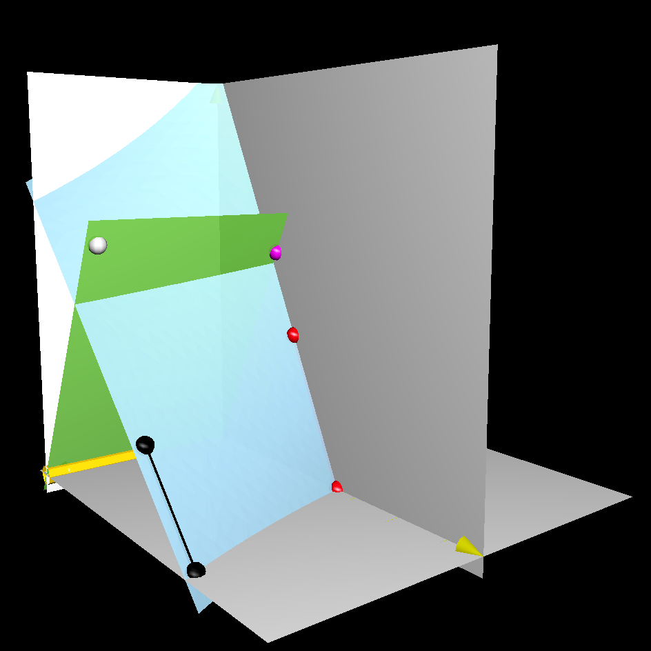
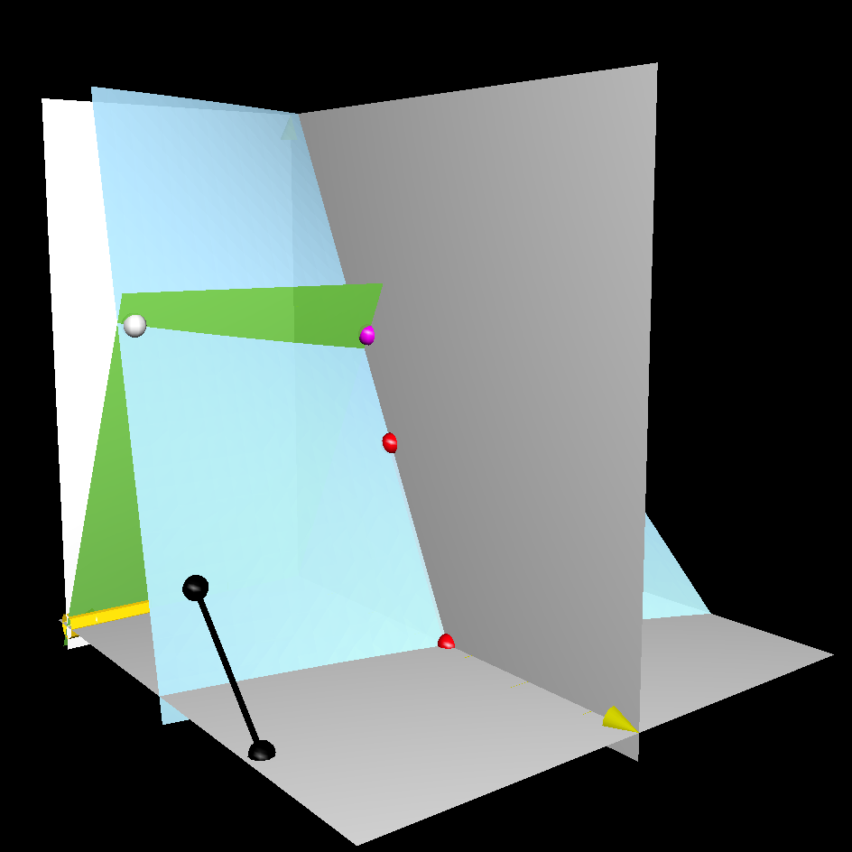
Hence . The proof is complete. An illustration of the projection of on -space is given in Figure 2. ∎
Before we prove that is flow-invariant, we need to prove the following technical proposition.
Proposition 4.3.
If on , then
on
Proof.
If , the by (2.17), we have
| (4.5) |
Since and in , we can drop terms with above. The computation continues as
| (4.6) |
Since , we know that
in if holds. Moreover, the inequality above implies
as Hence
Therefore.
on . ∎
Lemma 4.4.
The compact set is flow-invariant.
Proof.
We have two check three inequalities in . Firstly, we have
| (4.7) |
Note that is equivalent to in . We have
| (4.8) |
As for inequalities concerning ’s, we have
| (4.9) |
Finally, we have
| (4.10) |
By Proposition 4.3, the computation result above is non-negative. The proof is complete. ∎
By looking into the linearization of (2.20) at , and in Section 3. We learn that is in initially for ; is in initially for ; is in initially for for some . Therefore, all these integral curves are defined on . It is clear that in . Hence by Proposition 2.9, we obtain the following lemma, using the same notation for the integral curve and the metric represented.
Lemma 4.5.
The following metrics are complete.
-
1.
Smooth metrics , , defined on ;
-
2.
Smooth metrics , defined on ;
-
3.
Singular metrics with defined on
5 Asymptotics
We divide this section into two parts. We first study the asymptotics for the Ricci-flat metrics obtained in Theorem 1.1-1.3. Then we study the asymptotics for the negative Einstein metrics. Without further specifying, we use to denote any of the Einstein metrics in Lemma 4.5. A general property for a is the following.
Proposition 5.1.
All ’s are positive along each .
Proof.
By the definition of , we know that along each of the integral curves. It is also clear that ’s are non-negative in . Suppose reaches zero for some along . Then at that point we have
a contradiction. Similar argument can be used to prove that must be positive along . ∎
5.1 Asymptotics for Ricci-flat Metrics
All discussion in this section is restricted on , where the function vanishes. In the case , the asymptotic limit for was rigorously proven to be ALC by [Baz07]. In this section, we provide another proof and generalize the result for .
Proof.
Since along each of the integral curves, we know that decreases to some along . Suppose , then there exists some sequence with that .
On the other hand, we claim that there exists some such that along . Suppose not, then there exists some sequence with such that
Therefore, for the same sequence , it is necessary that
Since on , we conclude that there exists a point in the -limit set of of the form , with and . Such a point is a critical point of type 6 as in Section 3. It is clear that one of and must be negative, a contradiction to Proposition 5.1.
Observe (4.2), we can find a small enough such that implies
| (5.1) |
Hence stays positive and does not tend to zero along . We reach a contradiction. The limit for must be .
Note that is positive initially along each . Suppose for the first time at some , then at we have
| (5.2) |
By the identity , we have
| (5.3) |
Since by Proposition 5.1, the first term of the computation above is no larger than for any fixed . Hence we have
| (5.4) |
by replacing with in (5.3). As in , it is clear that . Hence we know that at . Then (5.2) continues as
| (5.5) |
Hence along . As , we must have . ∎
Remark 5.3.
The Böhm functional introduced in [Böh99] becomes and it is clear that
Since converges to , the functional blow up at infinity instead of converging to a finite number. This brings up a difficulty in describing the -limit set, which does not occur in two-summand case. One may consider the Böhm functional for the two-summand type subsystem on . However, the functional only demonstrate monotonicity in the subsystem.
Asymptotic limit for integral curves of two-summand type are known [Win17][Chi19a]. For , we know that . As for , we have the following.
Lemma 5.4.
For all , we have .
Proof.
In order to study the asymptotics of the other integral curves of Ricci-flat metrics, we need the following propositions.
Proposition 5.5.
Proof.
Fix any . Let and . We know that and are positive since is in . Note that
| (5.7) |
It is straightforward to check that coefficients of and above are positive at . Hence we can find a neighborhood around in which coefficients of and above are positive. If , then we see that must be positive. ∎
Proof.
Suppose the function vanishes finitely many times along . Then it eventually has a sign. Since , the function eventually monotonic decreases or increases. Hence for some . If , then we must have . By Proposition 5.2, we conclude that , where . But then one of and must be negative, a contradiction to Proposition 5.1. Hence we must have . Then we learn that the -limit set of contains some element in . Suppose were in the -limit set. Then converges to . Since is the minimum value for in and is assumed to have a sign eventually, we know that must be negative eventually. Consider
| (5.8) |
Since tends to and it is clear that in , is eventually positive along . Hence eventually monotonic increases. Then we conclude that has to converge to . But that implies eventually enters the set constructed in Proposition 5.5 and does not come out, which means that the function cannot converges to zero along . Hence we reach a contradiction. Therefore, is in the -limit set of . Since the point is a sink in , we have .
Suppose the function vanishes infinitely many times along . Then it is necessary that the function changes sign infinitely many times along . But
and converges to by Proposition 5.2. Hence there exists a sequence with such that and for each . Therefore, combining Proposition 5.1, the -limit set of must contain some point in the set
If , then converges to since the point is a sink in the subsystem restricted on . Suppose , then it is not a critical point. Since is a -dimensional invariant set and the -limit set is flow-invariant, the -limit set of must contain the integral curve that contains and lies on . Note that the reduced system on is essentially the two-summand type cohomogeneity one system. Based on the study in [Win17][Chi19a], we know that must converges to . Specifically, recall Remark 5.3 and consider the Böhm functional . We have
when restricted on . Hence increases monotonically to some positive number along , and the -limit set of contains some element in . Since is in the boundary of the 2-dimensional invariant set while is in the interior, one can exclude by perturbing the boundary of . Hence converges to and therefore is in the -limit set of . The proof is complete. ∎
The asymptotic limits of all integral curves that represent Ricci-flat metrics are known, as summarized in the following lemma.
Lemma 5.7.
Asymptotic limits of integral curves in Lemma 4.5 are the following.
| (5.9) |
5.2 Asymptotics for Negative Einstein metrics
Proposition 5.8.
Points in with must lie in the 1-dimensional stable manifold .
Proof.
By the definition of the function , we have in . Since is held, we obtain the lower bound for using Cauchy–Schwarz inequality. We have
| (5.10) |
Hence in But by the assumption on the point, we have . Hence we are forced to have and . Then is forced to vanish at such a point. The point must lie in . ∎
Lemma 5.9.
Let be any of integral curves with , with or in Lemma 4.5 with . We have for some .
Proof.
Since these integral curves are trapped in , we have as in (5.10). Then . Hence the function is increasing along and converges to some positive number. Then there exists a sequence with such that . Therefore, some subset of is in the -limit set of these integral curves by Proposition 5.8. The proof is complete by Lemma 3.5. ∎
For and , we know that they converge to . We are yet to determine what point in that and converges to if . Note that although decreases in this case, it does not necessarily need to converge to zero.
6 Relation to Special Holonomy
In this section, we check the holonomy of Einstein metrics in Theorem 1.1-1.3. Some known results are recovered.
6.1 Negative Kähler–Einstein and Calabi–Yau
We recover Kähler–Einstein metrics with a complex structure in [DW98] that is preserved by the action of . Recall Remark 1.5 that . If is Kähler–Einstein, then the coadjoint orbit is Kähler for each . Consequently, the cohomogeneity one Kähler–Einstein condition boils down to
| (6.1) |
The second equation above is equivalent to the coadjoint orbit being Kähler. In the new coordinate with variables defined in (2.14), integral curves that represent Kähler–Einstein metrics must lie in
We check the following.
Proposition 6.1.
The set is invariant.
Proof.
It is clear that is invariant. If in , then in . Hence on , we can eliminate all ’s and in (2.17) and obtain the following.
| (6.2) |
On the other hand, we have
| (6.3) |
Hence is invariant. ∎
Hence is an 2-dimensional invariant set. It straightforward to check that only contains critical points , and listed in Section 3. The last two critical points are of type 7 in Section 3. Since does not contain , , , or any point on , no integral curve of Theorem 1.1-1.3 lies in .
One can check that there are integral curves emanating from . They represent Kähler–Einstein metrics constructed in [BB82][Bes08, Theorem 9.129]. In particular, is a 1-dimensional invariant set that contains and . The part that “joins” these two critical points is exactly the image of the integral curve that emanates from and tends to , representing a Calabi–Yau metric with a bolt and an AE limit.
6.2 Quaternionic Kähler and Hyper-Kähler
By [DS99], the existence of the triple of almost complex structures forces and to be linear function in and . Therefore, any integral curve that represents a hyperKähler metric or a quaternionic Kähler metric must lie in the invariant set . For a quaternionic Kähler metric with normalized Einstein constant , the closedness of the fundamental 4-form implies
| (6.4) |
Therefore, integral curves that represent quaternionic Kähler metrics must lie in the following set.
Proposition 6.2.
The set is invariant.
Proof.
It is clear that is invariant. Moreover, becomes in and in . Hence on , we can eliminate , and all ’s in (2.17) and obtain the following.
| (6.5) |
Note that by the definition of , we must have . Hence computation above implies
on .
On the other hand, we have
| (6.6) |
and
| (6.7) |
Therefore the proof is complete. ∎
Critical points and are in the set and the set is 1-dimensional. The quaternionic Kähler metric in [Swa91] is realized as the integral curve . At the infinity, the exponential index for and is twice the one of . As in , we know that such an integral curve is not contained in hence it is not any one of the metrics in Theorem 1.1-1.3. Note that the hyper-Kähler metric is represented by the critical point , which is the flat metric on .
6.3
In the case , it is known that there exists metrics on and [CGLP04]. From [Hit01][CGLP04], we can write down the condition.
| (6.8) |
Define
| (6.9) |
The condition (6.8) is transformed to in the new coordinates. Define
We can check the following.
Proposition 6.3.
The set is invariant.
Proof.
On , we have
| (6.10) |
Computations show the above all vanish on . The proof is complete. ∎
Although the definition of consists of 6 equalities, one can show that holds once all ’s and vanish. Therefore, is a -dimensional surface and its projection to the -space is a level set given by
By changing the sign of . we obtain the condition with the opposite chirality.
| (6.11) |
and
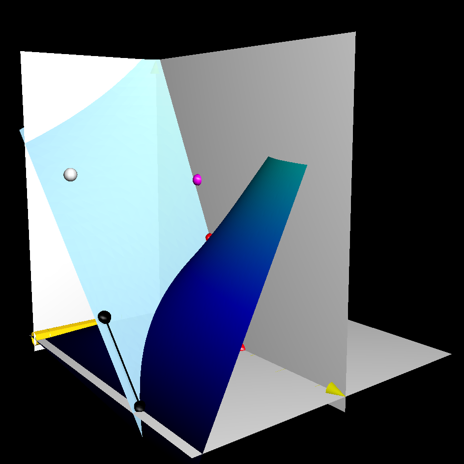
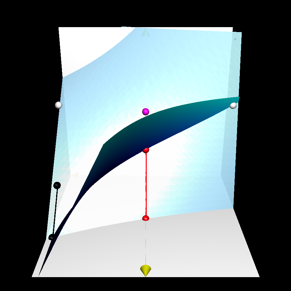
With the similar computation in the proof of Proposition 6.3, we can show that is invariant. Both invariant sets are presented in Figure 3. In our new coordinate, the metric and the metric in [BS89][GPP90] are realized as straight line segments that lie in .
Linearization at shows that lie in for all with and . is the AC metric found in [BS89][GPP90] and the 1-parameter family with is the family of ALC metrics found in [CGLP04]. Specifically, for we obtain
Another new metric was found on in [CGLP04]. This metric is locally the same as although they differ globally. This property is reflected in our pictures as both metrics are lie in the 1-dimensional invariant set
Simply change the sign of , then we can present with the opposite chirality in the compact invariant set . It is realized by the integral curve .
Remark 6.4.
In [CGLP02], the sign change occurs in one of the component in order to obtain non-trivially different system since is not necessarily . A 1-parameter family of metric was found in [CGLP02]. They are metrics with Fubini–Study bolt. At the infinity, one of the component tends to a constant while the other grow linearly as the same rate as . Therefore, these metrics are not realized in this article as the 3-sphere is really controlled by three functions instead of two. However, if one further impose , then the metric is the Calabi–Yau metrics described in Section 6.1.
Recall in Section 3.2, we know that there exists a unique unstable eigenvector of that is tangent to and emanates from via this vector. Computation shows that this eigenvector is tangent to . Hence is a singular metric.
In general, we have the following Lemma.
Lemma 6.5.
Consider the case . Metrics and on and metrics on all have holonomy group no smaller than . In particular,
-
1.
Metrics and on are .
-
2.
Metrics on is .
-
3.
Metrics with on have generic holonomy.
For the case , metrics with and on and metrics with on have generic holonomy.
Proof.
Consider the case . By the discussion above, it is clear that metrics and on , metrics on are . It suffices to prove with on have generic holonomy. By Lemma 5.7, we know that
Hence the limit space is one of the following.
-
1.
The metric cone over Jensen 7-sphere, its holonomy is .
-
2.
An -bundle over the metric cone over a nearly Kähler , whose holonomy group contains a subgroup .
-
3.
An -bundle over the metric cone over a Fubini–Study . The holonomy group contains a subgroup .
Suppose the metric admits a Kähler structure. By passing the Kähler structure to the limit space, we learn that the holonomy group of the limit space must be contained in .
Note that is -dimensional and simply connected. Both and have dimension larger than 15, hence they are not contained in . If the holonomy group that contains were also contained in , then it must be itself. But if were contained in , then must be a circle, a contradiction to the fact that is simply connected. We conclude that is not contained in . Therefore, with on must have generic holonomy.
Consider the case . With and Lemma 5.7, we have
Then the limit space must have holonomy group that contains a subgroup . Since the dimension of is larger than the one of if . We conclude that the Ricci-flat metrics above have generic holonomy. ∎
By Lemma 6.5 and by Theorem 2.1 in [Hit74] and [Wan89], Theorem 1.4 is proven.
Acknowledgements. The author is grateful to McKenzie Wang for introducing the problem and his useful comment. The author would like to thank Cheng Yang for helpful discussions on dynamic system. The author would also like to thank Christoph Böhm and Lorenzo Foscolo for their helpful suggestions and remarks on this project. Lemma 6.5 is proven thanks to the inspiring discussion with Lorenzo Foscolo.
References
- [Baz07] Ya. V. Bazaikin. On the new examples of complete noncompact Spin(7)-holonomy metrics. Siberian Mathematical Journal, 48(1):8–25, January 2007.
- [BB82] L. Bérard-Bergery. Sur de nouvelles variétés riemanniennes d’Einstein. In Institut Élie Cartan, 6, volume 6 of Inst. Élie Cartan, pages 1–60. Univ. Nancy, Nancy, 1982.
- [BDW15] M. Buzano, A.S. Dancer, and M.Y. Wang. A family of steady Ricci solitons and Ricci flat metrics. Comm. in Anal. and Geom., 23(3):611–638, 2015.
- [Bes08] A.L. Besse. Einstein Manifolds. Classics in Mathematics. Springer-Verlag, Berlin, 2008.
- [Böh99] C. Böhm. Non-compact cohomogeneity one Einstein manifolds. Bulletin de la Société Mathématique de France, 127(1):135–177, 1999.
- [BS89] R.L. Bryant and S.M. Salamon. On the construction of some complete metrics with exceptional holonomy. Duke Mathematical Journal, 58(3):829–850, 1989.
- [Cal75] E. Calabi. A construction of nonhomogeneous Einstein metrics. Differential geometry (Proc. Sympos. Pure Math., Vol. XXVII, Stanford Univ., Stanford, Calif., 1973), Part 2, pages 17–24, 1975.
- [CGLP02] M. Cvetič, G.W. Gibbons, H. Lü, and C.N. Pope. Cohomogeneity One Manifolds of Spin(7) and Holonomy. Physical Review D, 65(10), May 2002.
- [CGLP04] M. Cvetič, G.W. Gibbons, H. Lü, and C.N. Pope. New cohomogeneity one metrics with Spin(7) holonomy. Journal of Geometry and Physics, 49(3-4):350–365, 2004.
- [Che11] D. Chen. Examples of Einstein manifolds in odd dimensions. Annals of Global Analysis and Geometry, 40(3):339–377, October 2011.
- [Chi19a] H. Chi. Cohomogeneity one Einstein metrics on vector bundles. PhD Thesis, McMaster University, 2019.
- [Chi19b] Hanci Chi. Invariant Ricci-flat metrics of cohomogeneity one with Wallach spaces as principal orbits. Annals of Global Analysis and Geometry, 56(2):361–401, September 2019.
- [CL55] E.A. Coddington and N. Levinson. Theory of Ordinary Differential Equations. McGraw-Hill Book Company, Inc., New York-Toronto-London, 1955.
- [DS99] Andrew Dancer and Andrew Swann. Quaternionic Kähler manifolds of cohomogeneity one. International Journal of Mathematics, 10(05):541–570, August 1999.
- [DS02] A.S. Dancer and Ian A.B. Strachan. Einstein metrics on tangent bundles of spheres. Classical Quantum Gravity, 19(18):4663–4670, 2002.
- [DW98] A.S. Dancer and M.Y. Wang. Kähler–Einstein metrics of cohomogeneity one. Mathematische Annalen, 312(3):503–526, November 1998.
- [DW09a] A.S. Dancer and M.Y. Wang. Non-Kähler expanding Ricci solitons. International Mathematics Research Notices. IMRN, (6):1107–1133, 2009.
- [DW09b] A.S. Dancer and M.Y. Wang. Some New Examples of Non-Kähler Ricci Solitons. Mathematical Research Letters, 16(2):349–363, 2009.
- [EW00] J.-H. Eschenburg and M.Y. Wang. The initial value problem for cohomogeneity one Einstein metrics. The Journal of Geometric Analysis, 10(1):109–137, 2000.
- [FHN18] L. Foscolo, M. Haskins, and J. Nordström. Infinitely many new families of complete cohomogeneity one -manifolds: analogues of the Taub-NUT and Eguchi-Hanson spaces. arXiv:1805.02612 [hep-th], May 2018.
- [GPP90] G.W. Gibbons, D.N. Page, and C.N. Pope. Einstein metrics on and bundles. Communications in Mathematical Physics, 127(3):529–553, 1990.
- [Hit74] N. Hitchin. Harmonic Spinors. Advances in Mathematics, 14(1):1–55, September 1974.
- [Hit01] N. Hitchin. Stable forms and special metrics. In Global differential geometry: the mathematical legacy of Alfred Gray (Bilbao, 2000), volume 288, pages 70–89. Contemp. Math., Amer. Math. Soc., Providence, RI, 2001.
- [Jen73] G.R. Jensen. Einstein metrics on principal fibre bundles. Journal of Differential Geometry, 8(4):599–614, 1973.
- [PP86] D. N. Page and C. N. Pope. Einstein metrics on quaternionic line bundles. Classical and Quantum Gravity, 3(2):249–259, March 1986.
- [Rei11] F. Reidegeld. Exceptional holonomy and Einstein metrics constructed from Aloff–Wallach spaces. Proceedings of the London Mathematical Society, 102(6):1127–1160, June 2011.
- [Swa91] A. Swann. Hyper-Kähler and quaternionic Kähler geometry. Mathematische Annalen, 289(3):421–450, 1991.
- [VZ20] L. Verdiani and W. Ziller. Smoothness Conditions in Cohomogeneity manifolds. arXiv:1804.04680 [math], August 2020.
- [Wan89] M.Y. Wang. Parallel spinors and parallel forms. Annals of Global Analysis and Geometry, 7(1):59–68, 1989.
- [Wan91] M.Y. Wang. Preserving parallel spinors under metric deformations. Indiana University Mathematics Journal, 40(3):815–844, 1991.
- [Win17] M. Wink. Cohomogeneity one Ricci Solitons from Hopf Fibrations. arXiv:1706.09712 [math], June 2017.
- [WW98] J. Wang and M.Y. Wang. Einstein metrics on -bundles. Mathematische Annalen, 310(3):497–526, March 1998.