This paper was converted on www.awesomepapers.org from LaTeX by an anonymous user.
Want to know more? Visit the Converter page.

Eigenvalue analysis of stress-strain curve of two-dimensional amorphous solids of dispersed frictional grains with finite shear strain

Daisuke Ishima1, Kuniyasu Saitoh2, Michio Otsuki3, and Hisao Hayakawa1 1Yukawa Institute for Theoretical Physics, Kyoto University,
Kitashirakawa-oiwake cho, Sakyo-ku, Kyoto 606-8502, Japan,
2Department of Physics, Faculty of Science, Kyoto Sangyo University,
Motoyama, Kamigamo, Kita-ku, Kyoto 603-8555, Japan,
3Graduate School of Engineering Science, Osaka University, Toyonaka, Osaka 560-8531, Japan
Abstract

The stress-strain curve of two-dimensional frictional dispersed grains interacting with a harmonic potential without considering the dynamical slip under a finite strain is determined by using eigenvalue analysis of the Hessian matrix. After the configuration of grains is obtained, the stress-strain curve based on the eigenvalue analysis is in almost perfect agreement with that obtained by the simulation, even if there are plastic deformations caused by stress avalanches. Unlike the naive expectation, the eigenvalues in our model do not indicate any precursors to the stress-drop events.

I Introduction

Amorphous materials consisting of dispersed repulsive grains, such as powders, colloids, bubbles, and emulsions, behave as fragile solids above jamming density Jaeger96 ; Durian95 ; Wyart05 ; Baule18 ; Liu98 . When we consider a response of such materials to an applied strain γ\gamma, the rigidity GG is independent of the strain in the linear response regime, whereas it exhibits softening in the nonlinear regime Nagamanasa14 ; Knowlton14 ; Kawasaki16 ; Leishangthem17 ; Bohy17 ; Ozawa18 ; Clark18 ; Boschan19 ; Singh20 ; Otsuki21 . Above the yielding points, there are some plastic events, such as stress avalanches in the collection of grains.

The Hessian matrix determined by the configuration of grains is commonly used for amorphous solids consisting of frictionless grains  Wyart05 ; WyarLettt05 ; Ellenbroek06 ; Lerner16 ; Gartner16 ; Bonfanti19 ; Baule18 ; Morse20 . To determine the rigidity, eigenvalue analysis of the Hessian matrix DeGiuli14 ; Mizuno16 ; Maloney04 ; Maloney06 ; Lemaitre06 ; Zaccone11 ; Palyulin18 , is commonly used, but we have only obtained semi-quantitative agreements between the theory and simulation so far Zaccone11 ; Palyulin18 . Recently, some researchers examined the applicability of the instantaneous normal mode analysis to systems that are not fully equilibrated and found qualitative agreement between the analysis and simulation Oyama21 ; Kriuchevskyi22 , although they could not get quantitatively accurate results. Some studies have suggested that the decrement of the non-zero smallest eigenvalue of the Hessian matrix with the strain is a precursor of an avalanche or stress drop near a critical strain γc\gamma_{c}  Maloney04 ; Maloney06 ; Manning11 ; Dasgupta12 ; Ebrahem20 . Correspondingly, some studies indicated that the rigidity GG and the stress σ\sigma should behave as GGreg1/γcγG-G_{\rm reg}\propto-1/\sqrt{\gamma_{c}-\gamma} and σσregγcγ\sigma-\sigma_{\rm reg}\propto\sqrt{\gamma_{c}-\gamma} near γc\gamma_{c}, where GregG_{\rm reg} and σreg\sigma_{\rm reg} are the regular parts of the rigidity and stress conversing to constants at γc\gamma_{c}, respectively Maloney04 ; Maloney06 ; Karmakar10PRL ; Richard20 .

In general, the frictional force between the grains cannot be ignored in physical situations. Because the frictional force generally depends on the contact history, Hessian analysis is not applicable to such systems. Thus, Chattoraj et al. adopted the Jacobian matrix instead of the Hessian matrix to discuss the stability of the configuration of frictional grains under strain Chattoraj19 . They performed eigenvalue analysis under athermal quasi-static shear processes and determined the existence of oscillatory instability originating from interparticle friction at a certain strain Chattoraj19 ; Chattoraj19E ; Charan20 . Moreover, some studies have performed an analysis of the Hessian matrix with the aid of an effective potential for frictional grains Somfai07 ; Henkes10 . Recently, Liu et al. suggested that Hessian matrix analysis with another effective potential can be used, even if slip processes exist Liu21 . Previous studies Somfai07 ; Henkes10 have reported that the friction between grains causes a continuous change in the functional form of the density of states (DOS), which differs from that of frictionless systems. So far, there have been few theoretical studies to determine the rigidity of the frictional grains.

In our previous study Ishima2022 , we developed an analysis of the Jacobian matrix to determine the rigidity of two-dimensional amorphous solids consisting of frictional grains interacting with the Hertzian force in the linear response to an infinitesimal strain. In the study, we ignore the dynamic friction caused by the slip processes of contact points. We found that there are two modes in the DOS for a sufficiently small tangential-to-normal stiffness ratio. Rotational modes exist in the region of low-frequency or small eigenvalues, whereas translational modes exist in the region of high-frequency or large eigenvalues. The rigidity determined by the translational modes is in good agreement with that obtained by the molecular dynamics simulations, whereas the contribution of the rotational modes is almost zero. Nevertheless, there are several shortcomings in the previous analysis. (i) The analysis can be used only in the linear response regime, where the base state is not influenced by the applied strain. (ii) As a result, we cannot discuss the behavior of plastic deformations or avalanches of grains. (iii) Even if we restrict our interest to the linear response regime, we cannot include the effect of tangential contact for the preparation of the initial configuration. (iv) We also ignored the effect of Coulomb’s slip between the contacted grains Ishima2022 .

The purpose of this study is to overcome the shortcomings of our previous study except for point (iv) Ishima2022 . Thus, we analyze a collection of two-dimensional grains interacting with repulsive harmonic potentials within the contact radius, without considering Coulomb’s slip between the grains. Owing to the special properties of the harmonic potential, the eigenvalue analysis of the Jacobian matrix becomes equivalent to that of the Hessian matrix. Subsequently, using the eigenvalue analysis of the Hessian matrix, we demonstrate that the theoretical rigidity under a large strain agrees with that obtained by the simulation.

The remainder of this paper is organized as follows. In Sec. II, we introduce the model to be analyzed in this study. In Sec. III, we summarize the theoretical framework for determining the rigidity of an amorphous solid consisting of frictional grains without considering Coulomb’s slip process. In Sec. IV, we present the results of the stress-strain relation obtained using the theory formulated in Sec. III. We also compare the theoretical results with the simulation results to demonstrate the relevancy of our theoretical analysis. In Sec. V, we summarize the obtained results and address future tasks to be solved. In Appendix A, we numerically demonstrate the absence of history-dependent tangential deformations in our system. In Appendix B, we explain the detailed behavior of the eigenvalue near the stress-drop points. In Appendix C, we present some detailed properties of the Hessian matrix in a harmonic system. In Appendix D, we present some properties of the Jacobian matrix in a harmonic system and demonstrate its equivalency to the Hessian matrix. Appendix E presents the detailed properties of rigidity.

II Model

Our system contains NN frictional circular disks embedded in a two-dimensional space. To prevent the system from crystallization, it contains an equal number of grains with diameters dd and d/1.4d/1.4 Luding01 . We assume that the mass of grain ii is proportional to di2d_{i}^{2}, where did_{i} is the diameter of ii-th grain. For later convenience, we introduce mm as the mass of grain having a diameter dd. In this study, xi,yix_{i},y_{i}, and θi\theta_{i} denote xx and yy components of the position of ii-th grain, and the rotational angle of the ii-th grain, respectively. We introduce the generalized coordinates of the ii-th grain as follow:

𝒒i:=(𝒓iT,i)T,\bm{q}_{i}:=(\bm{r}_{i}^{\textrm{T}},\ell_{i})^{\textrm{T}}, (1)

where 𝒓i:=(xi,yi)T\bm{r}_{i}:=(x_{i},y_{i})^{\textrm{T}}, i:=diθi/2\ell_{i}:=d_{i}\theta_{i}/2, and the superscript T denotes the transposition.

Let the force, and zz-component of the torque acting on the ii-th grain be 𝑭i:=(Fix,Fiy)T\bm{F}_{i}:=(F_{i}^{x},F_{i}^{y})^{\textrm{T}} and TiT_{i}, respectively. Then, the equations of motion of ii-th grain are expressed as

mid2𝒓idt2\displaystyle m_{i}\frac{d^{2}\bm{r}_{i}}{dt^{2}} =𝑭i,\displaystyle=\bm{F}_{i}, (2)
Iid2θidt2\displaystyle I_{i}\frac{d^{2}\theta_{i}}{dt^{2}} =Ti,\displaystyle=T_{i}, (3)

with mass mim_{i} and momentum of inertia Ii:=midi2/8I_{i}:=m_{i}d_{i}^{2}/8 of ii-th grain. In a system without volume forces, such as gravity, we can write

𝑭i\displaystyle\bm{F}_{i} =ji𝒇ijmiηD𝒓˙i,\displaystyle=\sum_{j\neq i}\bm{f}_{ij}-m_{i}\eta_{D}\dot{\bm{r}}_{i}, (4)
Ti\displaystyle T_{i} =jiTijIiηDθ˙i,\displaystyle=\sum_{j\neq i}T_{ij}-I_{i}\eta_{D}\dot{\theta}_{i}, (5)

where we have adopted the notation A˙:=dA/dt\dot{A}:=dA/dt for arbitrary variable AA such as A=𝒓iA=\bm{r}_{i} and θi{\theta}_{i}. Here, 𝒇ij\bm{f}_{ij} and TijT_{ij} are the force and zz-component of the torque acting on the ii-th grain from the jj-th grain, respectively. As a simplified description of the drag terms from the background fluid, ηD\eta_{D} is a damping constant uniformly acting on grains, and TijT_{ij} is given by

Tij=di2(nijxfijynijyfijx),\displaystyle T_{ij}=-\frac{d_{i}}{2}({n}_{ij}^{x}{f}_{ij}^{y}-{n}_{ij}^{y}{f}_{ij}^{x}), (6)

where we have introduced the normal unit vector between ii-th and jj-th grains as 𝒏ij:=𝒓ij/|𝒓ij|:=(𝒓i𝒓j)/|𝒓i𝒓j|\bm{n}_{ij}:=\bm{r}_{ij}/|\bm{r}_{ij}|:=(\bm{r}_{i}-\bm{r}_{j})/|\bm{r}_{i}-\bm{r}_{j}|. The force 𝒇ij\bm{f}_{ij} can be divided into the normal part 𝒇N,ij\bm{f}_{N,ij} and tangential part 𝒇T,ij\bm{f}_{T,ij} as

𝒇ij=(𝒇N,ij+𝒇T,ij)H(dij/2|𝒓ij|),\displaystyle\bm{f}_{ij}=(\bm{f}_{N,ij}+\bm{f}_{T,ij})H(d_{ij}/2-|\bm{r}_{ij}|), (7)

where dij:=di+djd_{ij}:=d_{i}+d_{j} and H(x)H(x) is Heaviside’s step function, taking H(x)=1H(x)=1 for x>0,x>0, and H(x)=0H(x)=0 otherwise. We assume that the contact force is expressed as

𝒇N,ij:\displaystyle\bm{f}_{N,ij}: =kNξN,ij𝒏ij,\displaystyle=k_{N}\xi_{N,ij}\bm{n}_{ij}, (8)
𝒇T,ij:\displaystyle\bm{f}_{T,ij}: =kTξT,ij𝒕ij,\displaystyle=k_{T}\xi_{T,ij}\bm{t}_{ij}, (9)

where kNk_{N} and kTk_{T} are the stiffness parameters of normal and tangential contacts, respectively. The contact force can be derived from the harmonic potential. In Eqs. (8) and  (9) we have introduced ξN,ij:=dij/2|𝒓ij|\xi_{N,ij}:=d_{ij}/2-|\bm{r}_{ij}| and

𝝃T,ij(t):\displaystyle\bm{\xi}_{T,ij}(t): =Cij(t)𝑑t𝒗T,ij(t)\displaystyle=\int_{C_{ij}(t^{\prime})}dt^{\prime}\bm{v}_{T,ij}(t^{\prime})
[(Cij(t)𝑑t𝒗T,ij(t))𝒏ij(t)]𝒏ij(t),\displaystyle\quad-\left[\left(\int_{C_{ij}(t^{\prime})}dt^{\prime}\bm{v}_{T,ij}(t^{\prime})\right)\cdot\bm{n}_{ij}(t)\right]\bm{n}_{ij}(t), (10)

where we have used

𝒗T,ij:=𝒓˙ij𝝃˙N,ij+𝒖ij(diθ˙i+djθ˙j)/2\displaystyle\bm{v}_{T,ij}:=\dot{\bm{r}}_{ij}-\dot{\bm{\xi}}_{N,ij}+\bm{u}_{ij}(d_{i}\dot{\theta}_{i}+d_{j}\dot{\theta}_{j})/2 (11)

with 𝒖ij:=(nijy,nijx)T\bm{u}_{ij}:=(n_{ij}^{y},-n_{ij}^{x})^{\textrm{T}}, 𝒕ij:=𝝃T,ij/|ξT,ij|\bm{t}_{ij}:=-\bm{\xi}_{T,ij}/|\xi_{T,ij}|, ξT,ij:=|𝝃T,ij|\xi_{T,ij}:=|\bm{\xi}_{T,ij}|, and the integration over the duration time of contact between ii-th and jj-th grains Cij(t)𝑑t\int_{C_{ij}(t^{\prime})}dt^{\prime} with the trajectory Cij(t)C_{ij}(t^{\prime}) of the contact point between ii-th and jj-th grains at tt^{\prime}. As shown in Appendix A, we have confirmed that the second term on the right-hand side (RHS) of Eq. (10) is zero for harmonic systems, although we do not have any mathematical proof for this statement thus far. For simplicity, we consider neither the effects of Coulomb’s slip in the tangential equation of motion nor the dissipative contact force, where the tangential forces 𝒇T,ijC\bm{f}_{T,ij}^{C} including the effect of Coulomb’s slip process, satisfy

𝒇T,ijC:={𝒇T,ij(𝒇T,ij<μ|𝒇N,ij|)μ|𝒇N,ij|𝒕ij(otherwise)\displaystyle\bm{f}_{T,ij}^{C}:=\left\{\begin{matrix}\bm{f}_{T,ij}&(\bm{f}_{T,ij}<\mu|\bm{f}_{N,ij}|)\\ \mu|\bm{f}_{N,ij}|\bm{t}_{ij}&(\textrm{otherwise})\end{matrix}\right. (12)

where μ\mu is the friction constant.

We impose the Lees-Edwards boundary conditions Lees72 ; Evans08 , where the direction parallel to the shear strain is the xx-direction. After generating a stable grain configuration via isotropic compression starting from a random configuration by using Eqs. (2)-(10) without strain (see detail in Ref. Ishima2022 ), we apply a step strain Δγ\Delta\gamma to all grains, where xx-coordinate of the position of the ii-th grain is shifted by an affine displacement Δxi(Δγ):=ΔγyiFB(0)\Delta x_{i}(\Delta\gamma):=\Delta\gamma y_{i}^{\textrm{FB}}(0). Here, the superscript FB denotes the force-balance (FB) state at which 𝑭i=𝟎\bm{F}_{i}=\bm{0} and Ti=0T_{i}=0 for arbitrary ii. As shown in Sec. III.1, the FB state is equivalent to the potential minimum for harmonic grains. Subsequently, the system is relaxed to an FB state. We further apply the step strain Δγ\Delta\gamma associated with the subsequent relaxation process again to obtain the state at 2Δγ2\Delta\gamma. By repeating this process, we can reach a deformed state with the strain γ\gamma.

The plastic deformations for a large γ\gamma depend on the choice of Δγ\Delta\gamma Morse20 . Moreover, the theoretical formulation assumes Δγ0\Delta\gamma\to 0. Therefore, we adopt the backtracking method Lerner09 ; Karmakar10PRE . If a plastic event is encountered under a fixed Δγin\Delta\gamma_{\rm in}, the system is restored to its original state without a plastic event. Subsequently, we apply a new strain, 0.1Δγin0.1\Delta\gamma_{\rm in}, to the system. Even if we encounter a plastic event with 0.1Δγin0.1\Delta\gamma_{\rm in}, we further examine the smaller step strain of 0.01Δγin0.01\Delta\gamma_{\rm in}. We repeat this procedure until we reach Δγ<ΔγTh\Delta\gamma<\Delta\gamma_{\rm Th} (see Appendix B).

We introduce the rate of nonaffine displacements for riFB,ζ(γ)r_{i}^{{\rm FB},\zeta}(\gamma) with ζ=x\zeta=x or yy and iFB(γ)\ell_{i}^{\rm FB}(\gamma) as:

dr̊iζ(γ)dγ:\displaystyle\frac{d\mathring{r}_{i}^{\zeta}(\gamma)}{d\gamma}: =limΔγ0riFB,ζ(γ+Δγ)riFB,ζ(γ)ΔγδζxyiFB(γ),\displaystyle=\lim_{\Delta\gamma\to 0}\frac{r_{i}^{\textrm{FB},\zeta}(\gamma+\Delta\gamma)-r_{i}^{\textrm{FB},\zeta}(\gamma)}{\Delta\gamma}-\delta_{\zeta x}y_{i}^{\textrm{FB}}(\gamma), (13)
d̊i(γ)dγ:\displaystyle\frac{d\mathring{\ell}_{i}(\gamma)}{d\gamma}: =limΔγ0iFB(γ+Δγ)iFB(γ)Δγ.\displaystyle=\lim_{\Delta\gamma\to 0}\frac{\ell_{i}^{\textrm{FB}}(\gamma+\Delta\gamma)-\ell_{i}^{\textrm{FB}}(\gamma)}{\Delta\gamma}. (14)

Our system is characterized by the generalized coordinate 𝒒(γ):=(𝒒1T(γ),𝒒2T(γ),,𝒒NT(γ))T\bm{q}(\gamma):=(\bm{q}_{1}^{\textrm{T}}(\gamma),\bm{q}_{2}^{\textrm{T}}(\gamma),\cdots,\bm{q}_{N}^{\textrm{T}}(\gamma))^{\textrm{T}}. The configuration in the FB state at strain γ\gamma is denoted by 𝒒FB(γ):=((𝒒1FB(γ))T,(𝒒2FB(γ))T,,(𝒒NFB(γ))T)T\bm{q}^{\textrm{FB}}(\gamma):=((\bm{q}_{1}^{\textrm{FB}}(\gamma))^{\textrm{T}},(\bm{q}_{2}^{\textrm{FB}}(\gamma))^{\textrm{T}},\cdots,(\bm{q}_{N}^{\textrm{FB}}(\gamma))^{\textrm{T}})^{\textrm{T}}. The shear stress σ(γ)\sigma(\gamma) at 𝒒FB(γ)\bm{q}^{\textrm{FB}}(\gamma) for one sample is given by:

σ(𝒒FB(γ))=12L2ij>i\displaystyle\sigma(\bm{q}^{\textrm{FB}}(\gamma))=-\frac{1}{2L^{2}}\sum_{i}\sum_{j>i} [fijx(𝒒FB(γ))rijy(𝒒FB(γ))\displaystyle\left[f_{ij}^{x}(\bm{q}^{\textrm{FB}}(\gamma))r_{ij}^{y}(\bm{q}^{\textrm{FB}}(\gamma))\right.
+fijy(𝒒FB(γ))rijx(𝒒FB(γ))].\displaystyle\ +\left.f_{ij}^{y}(\bm{q}^{\textrm{FB}}(\gamma))r_{ij}^{x}(\bm{q}^{\textrm{FB}}(\gamma))\right]. (15)

The rigidity gg for one sample is defined as

g\displaystyle g :=dσ(𝒒(γ))dγ|𝒒(γ)=𝒒FB(γ),\displaystyle:=\left.\frac{d\sigma(\bm{q}(\gamma))}{d\gamma}\right|_{\bm{q}(\gamma)=\bm{q}^{\textrm{FB}}(\gamma)}, (16)

where the differentiation on the RHS of Eq. (16) is defined as follows:

dσ(𝒒(γ))dγ|𝒒(γ)=𝒒FB(γ)\displaystyle\left.\frac{d\sigma(\bm{q}(\gamma))}{d\gamma}\right|_{\bm{q}(\gamma)=\bm{q}^{\textrm{FB}}(\gamma)}
:=limΔγ0σ(𝒒FB(γ+Δγ))σ(𝒒FB(γ))Δγ.\displaystyle\quad\quad\quad:=\lim_{\Delta\gamma\to 0}\frac{\sigma(\bm{q}^{\textrm{FB}}(\gamma+\Delta\gamma))-\sigma(\bm{q}^{\textrm{FB}}(\gamma))}{\Delta\gamma}. (17)

In the numerical calculation, we use a non-zero but sufficiently small Δγ\Delta\gamma for the evaluation of gg. Then, the averaged rigidity GG is defined as

G\displaystyle G :=g,\displaystyle:=\Braket{g}, (18)

where \langle\cdot\rangle is the ensemble average.

III Theoretical Analysis

In this section, we introduce Hessian matrix in Sec. III.1 and theoretical expressions of rigidity in Sec. III.2.

III.1 Hessian matrix for frictional grains

Because the Hessian matrix is equivalent to the Jacobian matrix for harmonic grains, as shown in Appendices C.1 and D.3, in this study, we adopt the Hessian matrix (\mathcal{H}), where the element is given by Saitoh19 :

ijαβ:=2δeij(𝒒(γ))qiαqjβ|𝒒(γ)=𝒒FB(γ),\displaystyle\mathcal{H}_{ij}^{\alpha\beta}:=\left.\frac{\partial^{2}\delta e_{ij}(\bm{q}(\gamma))}{\partial q_{i}^{\alpha}\partial q_{j}^{\beta}}\right|_{\bm{q}(\gamma)=\bm{q}^{\textrm{FB}}(\gamma)}, (19)

where α\alpha and β\beta are any of x,yx,y and \ell, while ii and jj express the grain indices. Here, we have introduced the effective potential energy δeij\delta e_{ij} between the contacted ii-th and jj-th grains as:

δeij:=kN2(δ𝒓ij𝒏ij)2+kT2δ𝒓ij,2,\displaystyle\delta e_{ij}:=\frac{k_{N}}{2}(\delta\bm{r}_{ij}\cdot\bm{n}_{ij})^{2}+\frac{k_{T}}{2}\delta\bm{r}_{ij,\perp}^{2}, (20)

where δ𝒓ij,\delta\bm{r}_{ij,\perp} is defined as

δ𝒓ij,:=δ𝒓ij(δ𝒓ij𝒏ij)𝒏ijδij×𝒏ij\displaystyle\delta\bm{r}_{ij,\perp}:=\delta\bm{r}_{ij}-(\delta\bm{r}_{ij}\cdot\bm{n}_{ij})\bm{n}_{ij}-\delta\bm{\ell}_{ij}\times\bm{n}_{ij} (21)

with

δ𝒓ij:\displaystyle\delta\bm{r}_{ij}: =δ𝒓iδ𝒓j,\displaystyle=\delta\bm{r}_{i}-\delta\bm{r}_{j}, (22)
δij:\displaystyle\delta\bm{\ell}_{ij}: =(δi+δj)𝒆z\displaystyle=(\delta\ell_{i}+\delta\ell_{j})\bm{e}_{z} (23)

under the virtual displacements δ𝒓i\delta\bm{r}_{i} and δi\delta\ell_{i} from the FB state at 𝒓iFB\bm{r}_{i}^{\rm FB} and iFB\ell_{i}^{\rm FB}, respectively.

The Hessian matrix introduced in Eq. (19) can be written as

=[111i1j1Ni1iiijiNj1jijjjNN1NiNjNN],\displaystyle\mathcal{H}=\left[\begin{matrix}\mathcal{H}_{11}&\cdots&\mathcal{H}_{1i}&\cdots&\mathcal{H}_{1j}&\cdots&\mathcal{H}_{1N}\\ \vdots&\ddots&\vdots&&\vdots&&\vdots\\ \mathcal{H}_{i1}&\cdots&\mathcal{H}_{ii}&\cdots&\mathcal{H}_{ij}&\cdots&\mathcal{H}_{iN}\\ \vdots&&\vdots&\ddots&\vdots&&\vdots\\ \mathcal{H}_{j1}&\cdots&\mathcal{H}_{ji}&\cdots&\mathcal{H}_{jj}&\cdots&\mathcal{H}_{jN}\\ \vdots&&\vdots&&\vdots&\ddots&\vdots\\ \mathcal{H}_{N1}&\cdots&\mathcal{H}_{Ni}&\cdots&\mathcal{H}_{Nj}&\cdots&\mathcal{H}_{NN}\end{matrix}\right], (24)

where ij\mathcal{H}_{ij} is a 3×33\times 3 submatrix of the Hessian \mathcal{H} for a pair of grains ii and jj satisfying:

ij=[ijxxijxyijxijyxijyyijyijxijyij].\displaystyle\mathcal{H}_{ij}=\left[\begin{matrix}\mathcal{H}_{ij}^{xx}&\mathcal{H}_{ij}^{xy}&\mathcal{H}_{ij}^{x\ell}\\ \mathcal{H}_{ij}^{yx}&\mathcal{H}_{ij}^{yy}&\mathcal{H}_{ij}^{y\ell}\\ \mathcal{H}_{ij}^{\ell x}&\mathcal{H}_{ij}^{\ell y}&\mathcal{H}_{ij}^{\ell\ell}\end{matrix}\right]. (25)

See Appendix C.1 for an explicit expression of each component of the Hessian matrix. Note that ijαβ=0\mathcal{H}_{ij}^{\alpha\beta}=0 if the ii-th and jj-th grains are not in contact with each other.

Because \mathcal{H} is a real symmetric matrix, its eigenvalues and eigenvectors are also real. Using the decomposition of the potential, the Hessian matrix can be divided into

ijαβ=N,ijαβ+T,ijαβ,\displaystyle\mathcal{H}_{ij}^{\alpha\beta}=\mathcal{H}_{N,ij}^{\alpha\beta}+\mathcal{H}_{T,ij}^{\alpha\beta}, (26)

where

N,ijαβ:\displaystyle\mathcal{H}_{N,ij}^{\alpha\beta}: =2δeN,ijα(𝒒(γ))qiαqjβ|𝒒(γ)=𝒒FB(γ),\displaystyle=\left.\frac{\partial^{2}\delta e_{N,ij}^{\alpha}(\bm{q}(\gamma))}{\partial q_{i}^{\alpha}\partial q_{j}^{\beta}}\right|_{\bm{q}(\gamma)=\bm{q}^{\textrm{FB}}(\gamma)}, (27)
T,ijαβ:\displaystyle\mathcal{H}_{T,ij}^{\alpha\beta}: =2δeT,ijα(𝒒(γ))qiαqjβ|𝒒(γ)=𝒒FB(γ)\displaystyle=\left.\frac{\partial^{2}\delta e_{T,ij}^{\alpha}(\bm{q}(\gamma))}{\partial q_{i}^{\alpha}\partial q_{j}^{\beta}}\right|_{\bm{q}(\gamma)=\bm{q}^{\textrm{FB}}(\gamma)} (28)

for iji\neq j and

N,ijαβ:\displaystyle\mathcal{H}_{N,ij}^{\alpha\beta}: =2δeN,ikα(𝒒(γ))qiαqiβ|𝒒(γ)=𝒒FB(γ),\displaystyle=\left.\frac{\partial^{2}\delta e_{N,ik}^{\alpha}(\bm{q}(\gamma))}{\partial q_{i}^{\alpha}\partial q_{i}^{\beta}}\right|_{\bm{q}(\gamma)=\bm{q}^{\textrm{FB}}(\gamma)}, (29)
T,ijαβ:\displaystyle\mathcal{H}_{T,ij}^{\alpha\beta}: =2δeT,ikα(𝒒(γ))qiαqiβ|𝒒(γ)=𝒒FB(γ)\displaystyle=\left.\frac{\partial^{2}\delta e_{T,ik}^{\alpha}(\bm{q}(\gamma))}{\partial q_{i}^{\alpha}\partial q_{i}^{\beta}}\right|_{\bm{q}(\gamma)=\bm{q}^{\textrm{FB}}(\gamma)} (30)

for i=ji=j. Here, we have introduced

δeN,ij:\displaystyle\delta e_{N,ij}: =kN2(δ𝒓ij𝒏ij)2,\displaystyle=\frac{k_{N}}{2}(\delta\bm{r}_{ij}\cdot\bm{n}_{ij})^{2}, (31)
δeT,ij:\displaystyle\delta e_{T,ij}: =kT2δ𝒓ij,2.\displaystyle=\frac{k_{T}}{2}\delta\bm{r}_{ij,\perp}^{2}. (32)

To determine the explicit expression of each component of the Hessian matrix, refer to Appendix C.1.

The eigenequation of the Hessian matrix \mathcal{H} is given by

|Φn\displaystyle\mathcal{H}\ket{\Phi_{n}} =λn|Φn,\displaystyle=\lambda_{n}\ket{\Phi_{n}}, (33)

where |Φn\ket{\Phi_{n}} is the right eigenvector corresponding to the nn-th eigenvalue λn\lambda_{n} of \mathcal{H}. Because the Hessian matrix is a real symmetric matrix, its left eigenequation is equivalent to its right eigenequation. Such properties remain unchanged even under the Lees-Edwards boundary conditions (see Appendix C.2). If all eigenstates are non-degenerate, |Φn\ket{\Phi_{n}} satisfies the orthonormal relation Φm|Φn=δmn\braket{\Phi_{m}}{\Phi_{n}}=\delta_{mn} with normalization Φn|Φn=1\braket{\Phi_{n}}{\Phi_{n}}=1, where Φn|Φn:=i=1Nα=x,y,(Φn,iα)2\braket{\Phi_{n}}{\Phi_{n}}:=\sum_{i=1}^{N}\sum_{\alpha=x,y,\ell}(\Phi_{n,i}^{\alpha})^{2}.

III.2 Expressions of the rigidity via eigenmodes

In this subsection, we consider the rigidity gg introduced in Eq. (18). See Appendix E for the detailed properties of gg.

Let us introduce 𝑭~i:=(F~ix,F~iy,F~i)T:=(Fix,Fiy,2Ti/di)T\tilde{\bm{F}}_{i}:=(\tilde{F}^{x}_{i},\tilde{F}^{y}_{i},\tilde{F}^{\ell}_{i})^{\rm T}:=(F^{x}_{i},F^{y}_{i},2T_{i}/d_{i})^{\rm T} and |F~(𝒒(γ))\ket{\tilde{F}(\bm{q}(\gamma))} as

|F~(𝒒(γ)):=[𝑭~1T(𝒒(γ)),𝑭~2T(𝒒(γ)),,𝑭~NT(𝒒(γ))]T.\displaystyle\ket{\tilde{F}(\bm{q}(\gamma))}:=[\tilde{\bm{F}}_{1}^{\textrm{T}}(\bm{q}(\gamma)),\tilde{\bm{F}}_{2}^{\textrm{T}}(\bm{q}(\gamma)),\cdots,\tilde{\bm{F}}_{N}^{\textrm{T}}(\bm{q}(\gamma))]^{\textrm{T}}. (34)

Because the FB state is the minimum state of the potential energy, as shown in Appendix C.1, |F~(𝒒(γ))|𝒒(γ)=𝒒FB(γ)\ket{\tilde{F}(\bm{q}(\gamma))}|_{\bm{q}(\gamma)=\bm{q}^{\textrm{FB}}(\gamma)} satisfies

|F~(𝒒(γ))|𝒒(γ)=𝒒FB(γ)=d|F~(𝒒(γ))dγ|𝒒(γ)=𝒒FB(γ)=|0,\displaystyle\left.\ket{\tilde{F}(\bm{q}(\gamma))}\right|_{\bm{q}(\gamma)=\bm{q}^{\textrm{FB}}(\gamma)}=\left.\frac{d\ket{\tilde{F}(\bm{q}(\gamma))}}{d\gamma}\right|_{\bm{q}(\gamma)=\bm{q}^{\textrm{FB}}(\gamma)}=\ket{0}, (35)

where |0\ket{0} is the ket vector containing 0 for all components.

Introducing

|dq̊dγ:=[dr̊1xdγ,dr̊1ydγ,d̊1dγ,,dr̊Nxdγ,dr̊Nydγ,d̊Ndγ]T,\displaystyle\Ket{\frac{d\mathring{q}}{d\gamma}}:=\left[\frac{d\mathring{r}_{1}^{x}}{d\gamma},\frac{d\mathring{r}_{1}^{y}}{d\gamma},\frac{d\mathring{\ell}_{1}}{d\gamma},\cdots,\frac{d\mathring{r}_{N}^{x}}{d\gamma},\frac{d\mathring{r}_{N}^{y}}{d\gamma},\frac{d\mathring{\ell}_{N}}{d\gamma}\right]^{\textrm{T}}, (36)

one can write

d|F~(𝒒(γ))dγ|𝒒(γ)=𝒒FB(γ)=|Ξ+~|dq̊dγ,\displaystyle\left.\frac{d\ket{\tilde{F}(\bm{q}(\gamma))}}{d\gamma}\right|_{\bm{q}(\gamma)=\bm{q}^{\textrm{FB}}(\gamma)}=-\ket{\Xi}+\tilde{\mathcal{H}}\Ket{\frac{d\mathring{q}}{d\gamma}}, (37)

where we have used Eqs. (13) and (14). The first and second terms on the RHS of Eq. (37) represent the strain derivatives of the forces for the contributions from the affine and nonaffine displacements, respectively. In Eq. (37) we have introduced |Ξ\ket{\Xi}, which is defined as:

|Ξ:=j[N,j1xxr1jyN,j1xyr1jyN,j1xr1jyN,jNxxrNjyN,jNxyrNjyN,jNxrNjy].\displaystyle\ket{\Xi}:=\sum_{j}\left[\begin{matrix}\mathcal{H}_{N,j1}^{xx}r_{1j}^{y}\\ \mathcal{H}_{N,j1}^{xy}r_{1j}^{y}\\ \mathcal{H}_{N,j1}^{x\ell}r_{1j}^{y}\\ \vdots\\ \mathcal{H}_{N,jN}^{xx}r_{Nj}^{y}\\ \mathcal{H}_{N,jN}^{xy}r_{Nj}^{y}\\ \mathcal{H}_{N,jN}^{x\ell}r_{Nj}^{y}\end{matrix}\right]. (38)

We have used ~\tilde{\mathcal{H}} in Eq. (37), which is defined as

~iiαβ\displaystyle\tilde{\mathcal{H}}_{ii}^{\alpha\beta} :={iix(α=,β=x)iiy(α=,β=y)iiαβ(otherwise)\displaystyle:=\left\{\begin{matrix}-\mathcal{H}_{ii}^{\ell x}&(\alpha=\ell,\ \beta=x)\\ -\mathcal{H}_{ii}^{\ell y}&(\alpha=\ell,\ \beta=y)\\ \mathcal{H}_{ii}^{\alpha\beta}&(\textrm{otherwise})\end{matrix}\right. (39)

and

~ijαβ\displaystyle\tilde{\mathcal{H}}_{ij}^{\alpha\beta} :={ijx(α=x,β=)ijy(α=y,β=)ijαβ(otherwise)\displaystyle:=\left\{\begin{matrix}-\mathcal{H}_{ij}^{x\ell}&(\alpha=x,\ \beta=\ell)\\ -\mathcal{H}_{ij}^{y\ell}&(\alpha=y,\ \beta=\ell)\\ \mathcal{H}_{ij}^{\alpha\beta}&(\textrm{otherwise})\end{matrix}\right. (40)

for iji\neq j. Note that T,ijαβ\mathcal{H}_{T,ij}^{\alpha\beta} or ~T,ijαβ\tilde{\mathcal{H}}_{T,ij}^{\alpha\beta} does not affect |Ξ\ket{\Xi}, because the affine displacements are instantaneously applied to the system as a step strain. Thus, the integral interval of the tangential displacement during the affine deformation is zero.

Expanding the nonaffine displacements by the eigenvectors of ~\tilde{\mathcal{H}} and using the fact that the left-hand side of Eq. (37) is zero, we obtain

|dq̊dγ=nΦ~n|Ξλ~n|Φ~n,\displaystyle\Ket{\frac{d\mathring{q}}{d\gamma}}=\sideset{}{{}^{{}^{\prime}}}{\sum}_{n}\frac{\braket{\tilde{\Phi}_{n}}{\Xi}}{\tilde{\lambda}_{n}}\ket{\tilde{\Phi}_{n}}, (41)

where λ~n\tilde{\lambda}_{n} and |Φ~n\ket{\tilde{\Phi}_{n}} are the nn-th eigenvalues of ~\tilde{\mathcal{H}}, and the eigenvector corresponding to λ~n\tilde{\lambda}_{n}, respectively. Here, n\sum_{n}\nolimits^{\prime} on the RHS of Eq. (41) excludes low-frequency modes for λ~nt02/m1012\tilde{\lambda}_{n}t_{0}^{2}/m\leq 10^{-12} to maintain the numerical accuracy. Note that |Φ~n\ket{\tilde{\Phi}_{n}} satisfies the orthonormal relation Φ~m|Φ~n=δmn\braket{\tilde{\Phi}_{m}}{\tilde{\Phi}_{n}}=\delta_{mn}, if all eigenstates are non-degenerate. The expression for dq̊/dγd\mathring{q}/d\gamma in Eq. (41) leads to a discontinuous change in dq̊/dγd\mathring{q}/d\gamma at a critical strain γc\gamma_{c} for a plastic event because the eigenvectors and eigenvalues are discontinuously changed at this point.

The rigidity is decomposed into two parts:

g:=gA+gNA,\displaystyle g:=g_{\textrm{A}}+g_{\textrm{NA}}, (42)

where gAg_{\textrm{A}} and gNAg_{\textrm{NA}} are the rigidities corresponding to the affine and nonaffine displacements, respectively, for one sample. With the aid of Eqs. (15), (18), and (40), the expressions for gAg_{\textrm{A}} and gNAg_{\textrm{NA}} can be obtained as:

gA:\displaystyle g_{\textrm{A}}: =14L2i,j(ij)rijy[rijyN,jixx+rijxN,jiyx],\displaystyle=\frac{1}{4L^{2}}\sum_{i,j(i\neq j)}r_{ij}^{y}\left[r_{ij}^{y}\mathcal{H}_{N,ji}^{xx}+r_{ij}^{x}\mathcal{H}_{N,ji}^{yx}\right], (43)
gNA:\displaystyle g_{\textrm{NA}}: =14L2i,j(ij)[ζ=x,y(rijy~ijxζ+rijx~ijyζ)dr̊ijζdγ\displaystyle=\frac{1}{4L^{2}}\sum_{i,j(i\neq j)}\Biggl{[}\sum_{\zeta=x,y}\left(r_{ij}^{y}\tilde{\mathcal{H}}_{ij}^{x\zeta}+r_{ij}^{x}\tilde{\mathcal{H}}_{ij}^{y\zeta}\right)\frac{d\mathring{r}_{ij}^{\zeta}}{d\gamma}
(rijy~ijx+rijx~ijy)d̊ijdγ],\displaystyle\quad\quad\quad\quad\quad\quad\quad\quad\quad-\left(r_{ij}^{y}\tilde{\mathcal{H}}_{ij}^{x\ell}+r_{ij}^{x}\tilde{\mathcal{H}}_{ij}^{y\ell}\right)\frac{d\mathring{\ell}_{ij}}{d\gamma}\Biggl{]}, (44)

where we have introduced

dr̊ijζdγ:\displaystyle\frac{d\mathring{r}_{ij}^{\zeta}}{d\gamma}: =dr̊iζdγdr̊jζdγ,\displaystyle=\frac{d\mathring{r}_{i}^{\zeta}}{d\gamma}-\frac{d\mathring{r}_{j}^{\zeta}}{d\gamma}, (45)
d̊ijdγ:\displaystyle\frac{d\mathring{\ell}_{ij}}{d\gamma}: =d̊idγ+d̊jdγ.\displaystyle=\frac{d\mathring{\ell}_{i}}{d\gamma}+\frac{d\mathring{\ell}_{j}}{d\gamma}. (46)

Substituting Eq. (41) into Eq. (44), gNAg_{\textrm{NA}} can be rewritten as

gNA\displaystyle g_{\textrm{NA}} =1L2nΦ~n|ΞΘ|Φ~nλ~n,\displaystyle=-\frac{1}{L^{2}}\sideset{}{{}^{{}^{\prime}}}{\sum}_{n}\frac{\braket{\tilde{\Phi}_{n}}{\Xi}\braket{\Theta}{\tilde{\Phi}_{n}}}{\tilde{\lambda}_{n}}, (47)

where we have introduced

Θ|:=12j[(r1jy~j1xx+r1jx~j1yx),(r1jy~j1xy+r1jx~j1yy),,(rNjy~jNxy+rNjx~jNyy),(rNjy~jNx+rNjx~jNy)].\displaystyle\bra{\Theta}:=\frac{1}{2}\sum_{j}\left[\left(r_{1j}^{y}\tilde{\mathcal{H}}_{j1}^{xx}+r_{1j}^{x}\tilde{\mathcal{H}}_{j1}^{yx}\right),\left(r_{1j}^{y}\tilde{\mathcal{H}}_{j1}^{xy}+r_{1j}^{x}\tilde{\mathcal{H}}_{j1}^{yy}\right),\ldots,\left(r_{Nj}^{y}\tilde{\mathcal{H}}_{jN}^{xy}+r_{Nj}^{x}\tilde{\mathcal{H}}_{jN}^{yy}\right),\left(r_{Nj}^{y}\tilde{\mathcal{H}}_{jN}^{x\ell}+r_{Nj}^{x}\tilde{\mathcal{H}}_{jN}^{y\ell}\right)\right]. (48)

The affine rigidity can be also expressed as

gA=1L2Y|Ξ,\displaystyle g_{\textrm{A}}=\frac{1}{L^{2}}\braket{Y}{\Xi}, (49)

where

Y|:=[y1,0,0,y2,0,0,,yN,0,0].\displaystyle\bra{Y}:=\left[y_{1},0,0,y_{2},0,0,\cdots,y_{N},0,0\right]. (50)

To verify the validity of the theoretical treatment, we introduce the theoretical stress σth(γ)\sigma^{\textrm{th}}(\gamma) with the aid of Eq.(42) as

σth(γ+Δγ):=σ(𝒒FB(γ))+g(γ)Δγ.\displaystyle\sigma^{\textrm{th}}(\gamma+\Delta\gamma):=\sigma(\bm{q}^{\textrm{FB}}(\gamma))+g(\gamma)\Delta\gamma. (51)

IV Results and discussion

We verify the validity of the shear modulus obtained by the eigenvalue analysis by comparing it with that obtained by the simulation. First, we have confirmed the quantitative accuracy of our analysis to obtain the rigidity in the linear response regime of our system (see Appendix E.2), as in Ref. Ishima2022 .

For the numerical FB condition, we use the condition |F~iα|<FTh|\tilde{F}_{i}^{\alpha}|<F_{\textrm{Th}} for arbitrary ii, where we adopt FTh=1.0×10¹⁴kNdF_{\textrm{Th}}=1.0\times 10^{-14}k_{N}d for the numerical calculation. In our simulation, we also adopt ηD=kN/m\eta_{D}=\sqrt{k_{N}/m}. In this study, we present the results for kT/kN=1k_{T}/k_{N}=1, the area fraction ϕ=0.90\phi=0.90, and Δγin=1.0×10⁴\Delta\gamma_{\rm in}=1.0\times 10^{-4} with the ensemble averages of 3030 samples, except for Appendix E.2. Note that the we analyze only the systems with ϕ=0.90\phi=0.90 which is sufficiently larger than the jamming density for a two-dimensional system. We ignore the effect of dissipation in the eigenequation because the velocity of each grain is sufficiently small to incur infinitesimal agitation from the FB state. The time step used for the simulation, Δt\Delta t, is set to Δt=1.0×10²t0\Delta t=1.0\times 10^{-2}t_{0} with t0:=m/kNt_{0}:=\sqrt{m/k_{N}}, and numerical integration is performed using the velocity Verlet method.

Refer to caption
Figure 1: A stress-strain curve for 0γ0.50\leq\gamma\leq 0.5 for one sample of the collection of grains (N=128N=128), which includes the theoretical results (line) and simulation results (filled symbols) under the conditionΔγTh=Δγin=104\Delta\gamma_{\textrm{Th}}=\Delta\gamma_{\textrm{in}}=10^{-4}. The inset is a close-up of the stress-strain curve in the vicinity of a stress-drop event.
Refer to caption
Figure 2: Stress-strain relations for ΔγTh=1.0×10⁴\Delta\gamma_{\textrm{Th}}=1.0\times 10^{-4} (blue circles) and ΔγTh=1.0×10⁸\Delta\gamma_{\textrm{Th}}=1.0\times 10^{-8} (red triangles) with N=128N=128.

Now, let us consider a nonlinear regime in which there are many plastic events caused by stress avalanches. Here, we regard an event as plastic if the condition (i) σ(γ)σ(γΔγ)<0\sigma(\gamma)-\sigma(\gamma-\Delta\gamma)<0 or (ii) G(γΔγ)G(γ)>1.0×10²kNG(\gamma-\Delta\gamma)-G(\gamma)>1.0\times 10^{-2}k_{N} is satisfied.

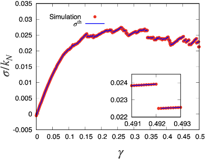
Figure 1 shows a typical example of the stress-strain curve obtained by one sample of the collection of grains based on both the simulation and eigenvalue analysis developed in the previous section under the condition ΔγTh=Δγin\Delta\gamma_{\rm Th}=\Delta\gamma_{\rm in}. It should be noted that the difference between the theoretical and simulation results is almost invisible, even in the presence of avalanches. However, the eigenvalue analysis cannot be used immediately after plastic events, that is, for γγc\gamma\approx\gamma_{c} (see the inset of Fig. 1), because the stress is not determined by Eq. (51) immediately after a plastic event.

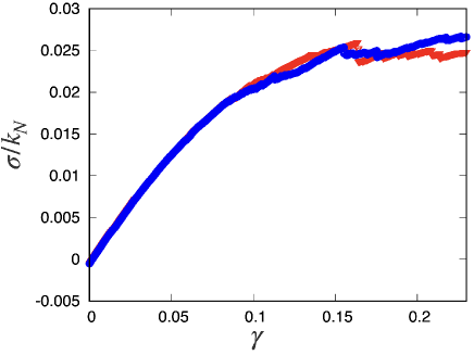
Figure 2 shows a comparison of the stress-strain curve for ΔγTh=104Δγin\Delta\gamma_{\rm Th}=10^{-4}\Delta\gamma_{\rm in} (blue circles) with those for ΔγTh=Δγin\Delta\gamma_{\rm Th}=\Delta\gamma_{\rm in} (red triangles). From the figure, we cannot find any ΔγTh\Delta\gamma_{\rm Th} dependence for γ<0.08\gamma<0.08, but some differences for larger γ\gamma can be observed as a result of stress avalanches.

Refer to caption
Refer to caption
Figure 3: Plots of (a) the smallest eigenvalue except for the zero modes and (b) the rigidity gg based on the eigenvalue analysis (open symbols) and numerical shear stress (filled symbols) against γ\gamma for 0.3408γ0.34130.3408\leq\gamma\leq 0.3413 and N=128N=128.

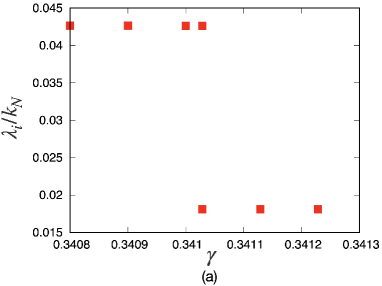
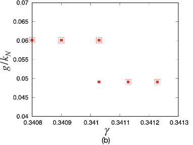
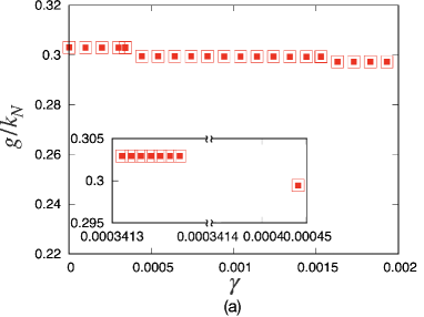
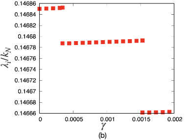
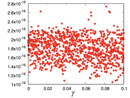
We might expect that some precursors of a stress-drop event can be detected from the behavior of the smallest non-zero eigenvalue. To verify this expectation, we plot the smallest non-zero eigenvalues in Fig. 3(a) near a critical strain with ΔγTh=108\Delta\gamma_{\rm Th}=10^{-8}. It can be observed that the eigenvalues changes discontinuously at the critical strain (γc=0.34102862\gamma_{c}=0.34102862 for γTh=108\gamma_{\rm Th}=10^{-8}), where the critical strain converges if ΔγTh<106\Delta\gamma_{\rm Th}<10^{-6} (see Appendix B for details). Notably, there is no precursor for the smallest eigenvalue below the critical strain, in contrast to Refs. Maloney04 ; Maloney06 ; Manning11 ; Dasgupta12 , where non-harmonic potentials are used. Correspondingly, we cannot find any singularity of the rigidity as ggreg(γcγ)1/2g-g_{\textrm{reg}}\sim-(\gamma_{c}-\gamma)^{-1/2} as in Fig. 3(b) for γγc\gamma\lesssim\gamma_{c} predicted in Refs. Maloney04 ; Maloney06 ; Karmakar10PRL ; Richard20 . The absence of the precursors and singularities in our model can be understood in the form of the Hessian matrix presented in Appendix D.3. In non-harmonic systems, some elements of the Hessian matrix become zero as ξN,ij0\xi_{N,ij}\to 0 when the contact between the ii-th and jj-th grains disappears. This leads to the precursors and singularities Maloney04 ; Maloney06 . However, in the harmonic systems, the corresponding element approaches a non-zero constant in the limit ξN,ij0\xi_{N,ij}\to 0 (see Appendix D.3), which results in the absence of the precursors.

Refer to caption
Refer to caption
Figure 4: Plots of eigenvectors at (a) γc\gamma_{c-} and at (b) γc+\gamma_{c+} corresponding to the smallest eigenvalue. For visualization, the magnitudes of the vectors are three times larger than their true values (N=1024N=1024).

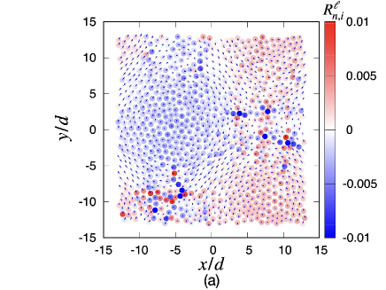
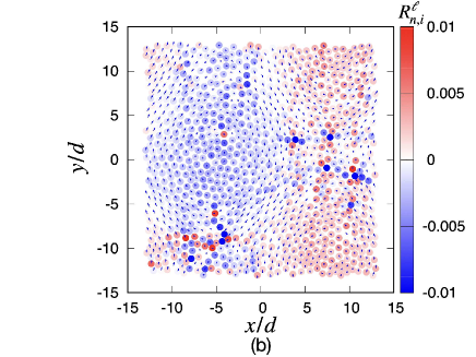
Figure 4 shows a set of plots of the eigenvectors corresponding to the smallest eigenvalue at (a) γc\gamma_{c-} and at (b)γc+\gamma_{c+}, where γc+\gamma_{c+} is the strain immediately after the plastic event, and γc:=γc+ΔγTh\gamma_{c-}:=\gamma_{c+}-\Delta\gamma_{\rm Th} is the strain just before the event. As shown in Fig. 4, changes in eigenvectors owing to the stress drop event can be observed. Here, we find the existence of domains of grains of clockwise rotation and counter-clockwise rotation, and the collective motion of grains between two domains. We may observe the excitation of the quadrupole-like mode, although its structure is not sufficiently clear.
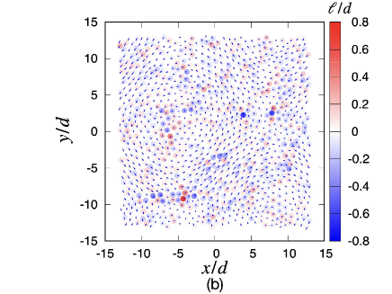
Figure 5 is the comparison of |dq̊/dγ\Ket{d\mathring{q}/d\gamma} obtained by the eigenvalue analysis (a) with that by the simulation (b) at γ=γc+\gamma=\gamma_{c+}, where |dq̊/dγ\Ket{d\mathring{q}/d\gamma} in the simulation is evaluated by (𝒒̊(γc++ΔγTh)𝒒̊(γc+))/ΔγTh(\mathring{\bm{q}}(\gamma_{c+}+\Delta\gamma_{\textrm{Th}})-\mathring{\bm{q}}(\gamma_{c+}))/\Delta\gamma_{\textrm{Th}} with ΔγTh=1.0×10⁸\Delta\gamma_{\textrm{Th}}=1.0\times 10^{-8}. It is obvious that the difference between the two figures is invisible, though the quadrupole-like structure cannot be clearly seen as in Fig. 4. Nevertheless, we can find the collective motion of grains in both figures.

Refer to caption
Refer to caption
Figure 5: Plots of |dq̊/dγ\Ket{d\mathring{q}/d\gamma} at γ=γc+\gamma=\gamma_{c+} for N=1024N=1024 and ΔγTh=1.0×10⁸\Delta\gamma_{\textrm{Th}}=1.0\times 10^{-8}, where (a) and (b) are based on the eigenvalue analysis and simulation, respectively. For visualization, we magnify the magnitudes of the vectors with the factor 10.010.0.
Refer to caption
Figure 6: Plot of Δq̊|c\Delta\mathring{q}|_{c} in the simulation for N=1024N=1024 and ΔγTh=1.0×10⁸\Delta\gamma_{\textrm{Th}}=1.0\times 10^{-8}. For visualization, we magnify Δq̊|c\Delta\mathring{q}|_{c} with the factor 1.0×1031.0\times 10^{3}.

Because we cannot use the eigenvalue analysis at the critical strain γc\gamma_{c} for a plastic event, let us analyze the nonaffine displacement Δ𝒒̊\Delta\mathring{\bm{q}} between γc\gamma_{c-} and γc+\gamma_{c+} caused by an avalanche using the simulation:

Δ𝒒̊|c:=[Δ𝒒̊1|cΔ𝒒̊2|cΔ𝒒̊N|c],\displaystyle\Delta\mathring{\bm{q}}|_{c}:=\left[\begin{matrix}\left.\Delta\mathring{\bm{q}}_{1}\right|_{c}\\ \left.\Delta\mathring{\bm{q}}_{2}\right|_{c}\\ \vdots\\ \left.\Delta\mathring{\bm{q}}_{N}\right|_{c}\end{matrix}\right], (52)

where

Δ𝒒̊i|c:=[riFB,x(γc+)riFB,x(γc)ΔγriFB,y(γc)riFB,y(γc+)riFB,y(γc)iFB(γc+)iFB(γc)].\displaystyle\left.\Delta\mathring{\bm{q}}_{i}\right|_{c}:=\left[\begin{matrix}r_{i}^{\textrm{FB},x}(\gamma_{c+})-r_{i}^{\textrm{FB},x}(\gamma_{c-})-\Delta\gamma r_{i}^{\textrm{FB},y}(\gamma_{c-})\\ r_{i}^{\textrm{FB},y}(\gamma_{c+})-r_{i}^{\textrm{FB},y}(\gamma_{c-})\\ \ell_{i}^{\textrm{FB}}(\gamma_{c+})-\ell_{i}^{\textrm{FB}}(\gamma_{c-})\end{matrix}\right]. (53)

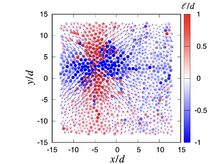
Figure 6 shows a plot of the nonaffine displacement Δ𝒒̊|c\Delta\mathring{\bm{q}}|_{c} around a yielding point based on the simulation for N=1024N=1024 at ΔγTh=1.0×10⁸\Delta\gamma_{\rm Th}=1.0\times 10^{-8}. This figure indicates that (i) grains move with rotations, which is one of the effects of mutual frictions between grains, and (ii) the existence of a quadrupole consisting of four domains of collective rotating grains exists. In particular, the rotations of the grains are sharply changed on the boundary between the domains. Unfortunately, Δ𝒒̊|c\Delta\mathring{\bm{q}}|_{c} cannot be described by the eigenvalue analysis, because Δ𝒒̊|c\Delta\mathring{\bm{q}}|_{c} expresses the configuration change, which is unstable for a small change in γ\gamma.

Refer to caption
Refer to caption
Figure 7: Plots of the shear modulus with (a) the theoretical evaluation (open symbols) and the simulation results (filled symbols) except for critical strain with the close-up of gg near a yielding point (inset), and (b) the smallest eigenvalue, except for zero modes against γ\gamma for 0γ0.0020\leq\gamma\leq 0.002 for N=128N=128. Note that the rigidity is not plotted at the yielding points, because it diverges there.

Figures 7 (a) and (b) show plots of the rigidity and smallest eigenvalue from γ=0\gamma=0 to 0.0020.002, which includes two plastic events based on the one-sample calculation of the collection of grains with N=128N=128. One can find an almost perfect agreement of the rigidity between the eigenvalue analysis and simulation, except for the yielding points (see Fig. 7 (a)). We find discontinuous changes in the smallest eigenvalue at the yielding point, where the rigidity changes discontinuously (see Fig.  7 (b). As expected, the magnitude of the discontinuous change in rigidity at the yielding point in Fig. 7 (a) for γ0.001\gamma\approx 0.001 is smaller than that for a point of a stress drop for γ0.341\gamma\approx 0.341, as shown in Fig. 3.

Refer to caption
Figure 8: The plot of the stress-strain curve in the region 0γ0.0020\leq\gamma\leq 0.002 for N=128N=128.

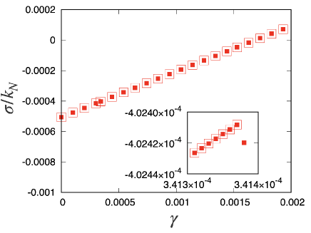
Figure 8 shows the stress-strain curve corresponding to Fig. 7. It is difficult to find the plastic events in the main figure of Fig. 8, but we can find a small stress drop at this point if we use a close-up figure in the inset. We verify the creation and annihilation of contacting pairs at the stress drop points. The stress expression in Eq. (51) cannot be used at the yielding point; thus a disagreement exists between the eigenvalue analysis and simulation at the point in the inset of Fig. 8.
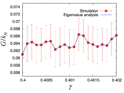
Refer to caption
Figure 9: Plots of the rigidity GG based on the eigenvalue analysis (line) and on the simulation (filled symbols) with ΔγTh=1.0×10⁴\Delta\gamma_{\textrm{Th}}=1.0\times 10^{-4}. We have used 3030 samples for N=128N=128, where the error bars represent the standard deviations for γ\gamma. Note that we have omitted the data if stress-drop events occur.

Figure 9 plots the rigidity of GG over 30 samples for N=128N=128, where we have omitted the data if stress drop events take place. We verify that rigidity based on the eigenvalue analysis reproduces the results of the simulation. Note that non-monotonic changes in GG originate from changes in the contact points and configuration of grains.

V Conclusion

In this paper, we have demonstrated that eigenvalue analysis of the Hessian matrix provides precise descriptions of the rigidity and stress of dispersed frictional grains in which the contact force is described by the harmonic potential, in spite of stress-drop events, such as stress avalanches. However, our model does not contain any slip processes between contacting grains. This success is a natural extension of the previous studies on frictionless grains Maloney04 ; Maloney06 to frictional grains and of our previous study on the linear response regime Ishima2022 to the nonlinear response regime. Two remarkable features of the contacting model are described by the harmonic potential. First, the tangential contact force in this model is no longer a history-dependent one. This leads to the significant simplification of the theoretical analysis. Second, unlike the naive expectation, the eigenvalues in our model do not indicate any precursors for the stress-drop events. In essence, stress-drop events take place suddenly by releasing contact points.

Some future tasks that need to be addressed are as follows. First, we need to consider the effect of slips, which causes a significant difference from our model because history-dependent contacts play important roles in the presence of slip events. Second, we must extend our analysis to nonlinear interacting models, such as the Hertzian contact model in a three-dimensional space. We plan on working on these points in the future.

VI ACKNOWLEDGMENTS

The authors thank N. Oyama for the fruitful discussions and useful comments. This work was partially supported by a Grant-in-Aid from the MEXT for Scientific Research (Grant No. JP22K03459, JP21H01006, and JP19K03670) and a Grant-in-Aid from the Japan Society for Promotion of Science JSPS Research Fellow (Grant No. JP20J20292).

Appendix A Absence of the second term on RHS of Eq. (10)

Refer to caption
Figure 10: Plot of the maximum Err against γ\gamma.

Thus far, we could not prove that the second term on RHS of Eq. (10) can be regarded as zero with numerical accuracy, but we verify that this term is zero, at least, in the numerical simulation of harmonic systems as follows: Let us calculate the ratio of the second term in Eq. (10) to the first term using

Err:=|[(Cij𝑑t𝒗T,ij)𝒏ij]𝒏ij||Cij𝑑t𝒗T,ij|.\displaystyle\textrm{Err}:=\frac{\left|\left[\left(\int_{C_{ij}}dt\bm{v}_{T,ij}\right)\cdot\bm{n}_{ij}\right]\bm{n}_{ij}\right|}{\left|\int_{C_{ij}}dt\bm{v}_{T,ij}\right|}. (54)

Figure 10 shows the plots of the largest Err in contacting pairs against γ\gamma, which indicates |Err|<3×10¹⁶|{\rm Err}|<3\times 10^{-16}. As our calculation is based on double precision, which has only 16 significant digits, Err can be regarded as zero.

Appendix B The behavior of the smallest eigenvalue near stress-drop points

In this appendix, we provide an in-depth explain the behavior of the smallest eigenvalue in the vicinity of the stress-drop points in detail. We adopt the following protocol to reduce the step strain small in the vicinity of the stress-drop point. We adopt Δγin=104\Delta\gamma_{\rm in}=10^{-4} in the appendix. We use Δγ=Δγin\Delta\gamma=\Delta\gamma_{\rm in} if there is no plastic event during the strain increment Δγ\Delta\gamma. If we find a stress drop during the strain from γ\gamma to γ+Δγ\gamma+\Delta\gamma, we restore the system to the state γ\gamma, and examine γ+0.1Δγin\gamma+0.1\Delta\gamma_{\rm in}. If we do not find any stress drop, we further add the strain with Δγin\Delta\gamma_{\rm in}; if we still have a stress drop, we repeat the procedure of restoring and adding strain 0.01Δγin0.01\Delta\gamma_{\rm in}. This protocol is repeated to detect stress drop events until we reach Δγ<ΔγTh\Delta\gamma<\Delta\gamma_{\rm Th}. In this appendix, we illustrate how the results depend on the choice of ΔγTh\Delta\gamma_{\rm Th}, where the smallest value of ΔγTh\Delta\gamma_{\rm Th} is 101010^{-10}.

Figure 11 presents the stress-strain curves obtained using this protocol. The upper branch in Fig. 11 represents the shear stress below the stress drop, and the lower branch represents the shear stress above the stress drop. The smallest γ\gamma in the lower branch and the largest γ\gamma in the upper branch strongly depend on ΔγTh\Delta\gamma_{\rm Th}. As shown in Fig. 12, the stress drop takes place at γ0.01330\gamma\approx 0.01330 for ΔγTh=104\Delta\gamma_{\rm Th}=10^{-4}, whereas the critical strain γc\gamma_{c} for the stress drop approaches 0.013334 as ΔγTh\Delta\gamma_{\rm Th} decreases, where γc\gamma_{c} is 0.013334 for ΔγTh106\Delta\gamma_{\rm Th}\leq 10^{-6}.

Refer to caption
Figure 11: The stress-strain curve for N=128N=128, which are the stress drop points for various ΔγTh\Delta\gamma_{\rm Th} (from ΔγTh=104\Delta\gamma_{\rm Th}=10^{-4} and ΔγTh=1010\Delta\gamma_{\rm Th}=10^{-10}).
Refer to caption
Figure 12: Plot of the critical strain γc\gamma_{c} against ΔγTh\Delta\gamma_{\rm Th} for N=128N=128.

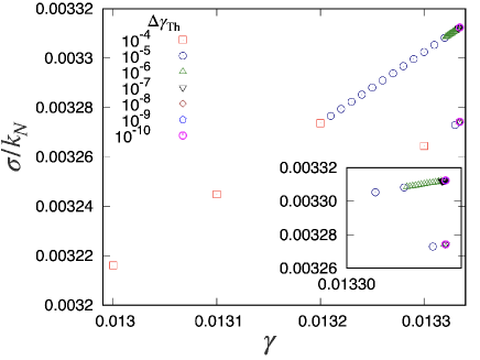
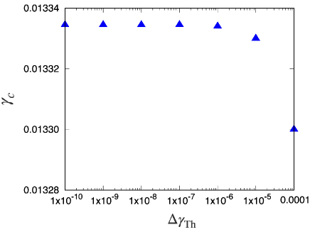
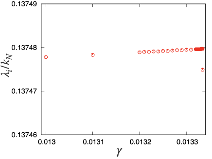
Figure 13 plots the behavior of the smallest eigenvalue against γ\gamma corresponding to Fig. 11 for ΔγTh=1010\Delta\gamma_{\rm Th}=10^{-10} immediately below the stress drop point, where the symbols correspond to the analysis for the corresponding Δγ\Delta\gamma as in Fig. 11. We have confirmed that there is no precursor of the eigenvalues below γc\gamma_{c} as observed in Hertzian and Lennard-Jones systems Maloney04 ; Maloney06 ; Manning11 . Thus, the harmonic system does not have any precursors in the behavior of the smallest eigenvalue.

Refer to caption
Figure 13: The plot of the smallest non-zero eigenvalue in the vicinity of γc\gamma_{c} for ΔγTh=1.0×10¹⁰\Delta\gamma_{\rm Th}=1.0\times 10^{-10}.

Appendix C Some properties of the Hessian matrix in a harmonic system

In this appendix, we briefly summarize the properties of the Hessian matrix of the harmonic contact model. In Sec. C.1, we explicitly express the elements of the Hessian matrix in this model. In Sec. C.2, we demonstrate that the symmetry of the Hessian matrix still holds even under the Lees-Edwards boundary condition.

C.1 The explicit expression for the Hessian matrix

In this appendix, we present an explicit expression for the Hessian matrix. To this end, we return to the effective potential in Eq. (20). It is straightforward to obtain

2δ𝒓ij,2xi2\displaystyle\frac{\partial^{2}\delta\bm{r}_{ij,\perp}^{2}}{\partial x_{i}^{2}} =22(nijx)2,\displaystyle=2-2(n_{ij}^{x})^{2}, (55)
2δ𝒓ij,2xiyi\displaystyle\frac{\partial^{2}\delta\bm{r}_{ij,\perp}^{2}}{\partial x_{i}\partial y_{i}} =2nijxnijy,\displaystyle=-2n_{ij}^{x}n_{ij}^{y}, (56)
2δ𝒓ij,2xii\displaystyle\frac{\partial^{2}\delta\bm{r}_{ij,\perp}^{2}}{\partial x_{i}\partial\ell_{i}} =2nijy,\displaystyle=2n_{ij}^{y}, (57)
2δ𝒓ij,2yixi\displaystyle\frac{\partial^{2}\delta\bm{r}_{ij,\perp}^{2}}{\partial y_{i}\partial x_{i}} =2δ𝒓ij,2xiyi,\displaystyle=\frac{\partial^{2}\delta\bm{r}_{ij,\perp}^{2}}{\partial x_{i}\partial y_{i}}, (58)
2δ𝒓ij,2yi2\displaystyle\frac{\partial^{2}\delta\bm{r}_{ij,\perp}^{2}}{\partial y_{i}^{2}} =22(nijy)2,\displaystyle=2-2(n_{ij}^{y})^{2}, (59)
2δ𝒓ij,2yii\displaystyle\frac{\partial^{2}\delta\bm{r}_{ij,\perp}^{2}}{\partial y_{i}\partial\ell_{i}} =2nijx,\displaystyle=2n_{ij}^{x}, (60)
2δ𝒓ij,2ixi\displaystyle\frac{\partial^{2}\delta\bm{r}_{ij,\perp}^{2}}{\partial\ell_{i}\partial x_{i}} =2δ𝒓ij,2xii,\displaystyle=\frac{\partial^{2}\delta\bm{r}_{ij,\perp}^{2}}{\partial x_{i}\partial\ell_{i}}, (61)
2δ𝒓ij,2iyi\displaystyle\frac{\partial^{2}\delta\bm{r}_{ij,\perp}^{2}}{\partial\ell_{i}\partial y_{i}} =2δ𝒓ij,2yii,\displaystyle=\frac{\partial^{2}\delta\bm{r}_{ij,\perp}^{2}}{\partial y_{i}\partial\ell_{i}}, (62)
2δ𝒓ij,2i2\displaystyle\frac{\partial^{2}\delta\bm{r}_{ij,\perp}^{2}}{\partial\ell_{i}^{2}} =2.\displaystyle=2. (63)

Thus, we obtain

ijxx\displaystyle\mathcal{H}_{ij}^{xx} =2δeijxixj=2δeijxi2=kN+kN[1+ξN,ij|𝒓ij|](nijy)2kT(nijy)2,\displaystyle=\frac{\partial^{2}\delta e_{ij}}{\partial x_{i}\partial x_{j}}=-\frac{\partial^{2}\delta e_{ij}}{\partial x_{i}^{2}}=-k_{N}+k_{N}\left[1+\frac{\xi_{N,ij}}{|\bm{r}_{ij}|}\right](n_{ij}^{y})^{2}-k_{T}(n_{ij}^{y})^{2}, (64)
ijxy\displaystyle\mathcal{H}_{ij}^{xy} =2δeijxiyj=2δeijxiyi=kN[1+ξN,ij|𝒓ij|]nijxnijy+kTnijxnijy,\displaystyle=\frac{\partial^{2}\delta e_{ij}}{\partial x_{i}\partial y_{j}}=-\frac{\partial^{2}\delta e_{ij}}{\partial x_{i}\partial y_{i}}=-k_{N}\left[1+\frac{\xi_{N,ij}}{|\bm{r}_{ij}|}\right]n_{ij}^{x}n_{ij}^{y}+k_{T}n_{ij}^{x}n_{ij}^{y}, (65)
ijx\displaystyle\mathcal{H}_{ij}^{x\ell} =2δeijxij=2δeijxii=kTnijy,\displaystyle=\frac{\partial^{2}\delta e_{ij}}{\partial x_{i}\partial\ell_{j}}=\frac{\partial^{2}\delta e_{ij}}{\partial x_{i}\partial\ell_{i}}=k_{T}n_{ij}^{y}, (66)
ijyy\displaystyle\mathcal{H}_{ij}^{yy} =2δeijyiyj=2δeijyi2=kN+kN[1+ξN,ij|𝒓ij|](nijx)2kT(nijx)2,\displaystyle=\frac{\partial^{2}\delta e_{ij}}{\partial y_{i}\partial y_{j}}=-\frac{\partial^{2}\delta e_{ij}}{\partial y_{i}^{2}}=-k_{N}+k_{N}\left[1+\frac{\xi_{N,ij}}{|\bm{r}_{ij}|}\right](n_{ij}^{x})^{2}-k_{T}(n_{ij}^{x})^{2}, (67)
ijy\displaystyle\mathcal{H}_{ij}^{y\ell} =2δeijyij=2δeijyii=kTnijx,\displaystyle=\frac{\partial^{2}\delta e_{ij}}{\partial y_{i}\partial\ell_{j}}=\frac{\partial^{2}\delta e_{ij}}{\partial y_{i}\partial\ell_{i}}=-k_{T}n_{ij}^{x}, (68)
ij\displaystyle\mathcal{H}_{ij}^{\ell\ell} =2δeijij=2δeiji2=kT\displaystyle=\frac{\partial^{2}\delta e_{ij}}{\partial\ell_{i}\partial\ell_{j}}=\frac{\partial^{2}\delta e_{ij}}{\partial\ell_{i}^{2}}=k_{T} (69)

for iji\neq j and

iixx\displaystyle\mathcal{H}_{ii}^{xx} =ji2δeijxi2=ji[kN+kN[1+ξN,ij|𝒓ij|](nijy)2kT(nijy)2],\displaystyle=\sum_{j\neq i}\frac{\partial^{2}\delta e_{ij}}{\partial x_{i}^{2}}=-\sum_{j\neq i}\left[-k_{N}+k_{N}\left[1+\frac{\xi_{N,ij}}{|\bm{r}_{ij}|}\right](n_{ij}^{y})^{2}-k_{T}(n_{ij}^{y})^{2}\right], (70)
iixy\displaystyle\mathcal{H}_{ii}^{xy} =ji2δeijxiyi=ji[kN[1+ξN,ij|𝒓ij|]nijxnijy+kTnijxnijy],\displaystyle=\sum_{j\neq i}\frac{\partial^{2}\delta e_{ij}}{\partial x_{i}\partial y_{i}}=-\sum_{j\neq i}\left[-k_{N}\left[1+\frac{\xi_{N,ij}}{|\bm{r}_{ij}|}\right]n_{ij}^{x}n_{ij}^{y}+k_{T}n_{ij}^{x}n_{ij}^{y}\right], (71)
iix\displaystyle\mathcal{H}_{ii}^{x\ell} =ji2δeijxii=jikTnijy,\displaystyle=\sum_{j\neq i}\frac{\partial^{2}\delta e_{ij}}{\partial x_{i}\partial\ell_{i}}=\sum_{j\neq i}k_{T}n_{ij}^{y}, (72)
iiyy\displaystyle\mathcal{H}_{ii}^{yy} =ji2δeijyi2=ji[kN+kN[1+ξN,ij|𝒓ij|](nijx)2kT(nijx)2],\displaystyle=\sum_{j\neq i}\frac{\partial^{2}\delta e_{ij}}{\partial y_{i}^{2}}=\sum_{j\neq i}\left[-k_{N}+k_{N}\left[1+\frac{\xi_{N,ij}}{|\bm{r}_{ij}|}\right](n_{ij}^{x})^{2}-k_{T}(n_{ij}^{x})^{2}\right], (73)
iiy\displaystyle\mathcal{H}_{ii}^{y\ell} =ji2δeijyii=jikTnijx,\displaystyle=\sum_{j\neq i}\frac{\partial^{2}\delta e_{ij}}{\partial y_{i}\partial\ell_{i}}=-\sum_{j\neq i}k_{T}n_{ij}^{x}, (74)
ii\displaystyle\mathcal{H}_{ii}^{\ell\ell} =ji2δeiji2=jikT.\displaystyle=\sum_{j\neq i}\frac{\partial^{2}\delta e_{ij}}{\partial\ell_{i}^{2}}=\sum_{j\neq i}k_{T}. (75)

C.2 Effect of the boundary condition to the Hessian matrix

In this appendix, we explain the influence of strain and the boundary condition on the Hessian matrix in detail to determine whether the symmetry of the Hessian matrix is still maintained, even if we consider a system with non-zero strain.

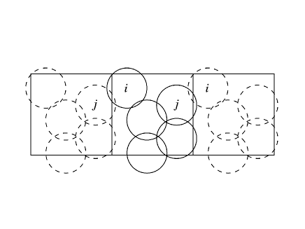
First, let us consider the case in which particle ii interacts with the particle jj through a mirror image in xx-direction, as shown in Fig. 14. In this case, 𝒓ij\bm{r}_{ij} is given by

𝒓ij:=𝒓i𝒓jL𝒆x,\displaystyle\bm{r}_{ij}:=\bm{r}_{i}-\bm{r}_{j}-L\bm{e}_{x}, (76)

where 𝒆x:=(1,0)T\bm{e}_{x}:=(1,0)^{\textrm{T}}. Similarly, 𝒓ji\bm{r}_{ji} is given by

𝒓ji:=𝒓j𝒓i+L𝒆x.\displaystyle\bm{r}_{ji}:=\bm{r}_{j}-\bm{r}_{i}+L\bm{e}_{x}. (77)

Thus, 𝒓ij\bm{r}_{ij} satisfies

𝒓ji=𝒓ij.\displaystyle\bm{r}_{ji}=-\bm{r}_{ij}. (78)

Then, we obtain

ξN,ij:\displaystyle\xi_{N,ij}: =di+dj2|𝒓ij|\displaystyle=\frac{d_{i}+d_{j}}{2}-|\bm{r}_{ij}|
=di+dj2|𝒓ji|\displaystyle=\frac{d_{i}+d_{j}}{2}-|\bm{r}_{ji}|
=ξN,ji.\displaystyle=\xi_{N,ji}. (79)

Thus, the result is independent of the strain, and the symmetry of the Hessian is still valid in this case.

Refer to caption
Figure 14: A schematic of the case where the particle ii interacts with the particle jj through the mirror image in xx-direction.

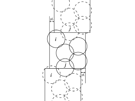
Next, let us consider the case in which the particle ii interacts with the particle jj through a mirror image in the yy-direction (see Fig. 15). In this case, 𝒓ij\bm{r}_{ij} is given by

𝒓ij:=𝒓i𝒓j+L𝒆y+γL𝒆x,\displaystyle\bm{r}_{ij}:=\bm{r}_{i}-\bm{r}_{j}+L\bm{e}_{y}+\gamma L\bm{e}_{x}, (80)

where 𝒆y:=(0,1)T\bm{e}_{y}:=(0,1)^{\textrm{T}}. Similarly, 𝒓ji\bm{r}_{ji} is given by

𝒓ji:=𝒓j𝒓iL𝒆yγL𝒆x.\displaystyle\bm{r}_{ji}:=\bm{r}_{j}-\bm{r}_{i}-L\bm{e}_{y}-\gamma L\bm{e}_{x}. (81)

Since the relation

𝒓ji=𝒓ij,\displaystyle\bm{r}_{ji}=-\bm{r}_{ij}, (82)

we obtain

ξN,ij:\displaystyle\xi_{N,ij}: =di+dj2|𝒓ij|\displaystyle=\frac{d_{i}+d_{j}}{2}-|\bm{r}_{ij}|
=di+dj2|𝒓ji|\displaystyle=\frac{d_{i}+d_{j}}{2}-|\bm{r}_{ji}|
=ξN,ji.\displaystyle=\xi_{N,ji}. (83)

Thus, ξN,ij\xi_{N,ij} and ξN,ji\xi_{N,ji} depend on γ\gamma in the same way. With the aid of Eqs. (80),(81) and (83), the Hessian matrix depends on γ\gamma if the particle interacts with another particle through the mirror image in yy-direction, although the symmetry of the Hessian is still maintained.

Refer to caption
Figure 15: A schematic of the case that the particle ii interacts with the particle jj through the mirror image in yy-direction.

Appendix D Some properties of the Jacobian matrix in a harmonic system and its equivalency to the Hessian matrix 

In this appendix, we briefly summarize the properties of the Jacobian matrix for the harmonic contact model that was previously used in the description of frictional grains Chattoraj19 ; Chattoraj19E ; Charan20 ; Ishima2022 . In Sec.D.1, we present explicit forms of the diagonal and non-diagonal blocks of the Jacobian matrix. In Sec.D.2, we present the derivation of the Jacobian for the harmonic contact model. In Sec. D.3, we explicitly write the elements of the Jacobian matrix in the model.

D.1 Jacobian block elements

Let us write a 3×33\times 3 sub-matrix 𝒥ij\mathcal{J}_{ij}, which is the (ij)(ij) block element of the Jacobian obtained from Eq. (19):

[𝒥ijαβ]\displaystyle\left[\mathcal{J}_{ij}^{\alpha\beta}\right] :=[F~iαqjβ]\displaystyle:=\left[-\frac{\partial\tilde{F}_{i}^{\alpha}}{\partial q_{j}^{\beta}}\right]
=[qjxFixqjyFixqjFixqjxFiyqjyFiyqjFiyqjxT~iqjyT~iqjT~i]\displaystyle=\left[\begin{matrix}-\partial_{q_{j}^{x}}F_{i}^{x}&-\partial_{q_{j}^{y}}F_{i}^{x}&-\partial_{q_{j}^{\ell}}F_{i}^{x}\\ -\partial_{q_{j}^{x}}F_{i}^{y}&-\partial_{q_{j}^{y}}F_{i}^{y}&-\partial_{q_{j}^{\ell}}F_{i}^{y}\\ -\partial_{q_{j}^{x}}\tilde{T}_{i}&-\partial_{q_{j}^{y}}\tilde{T}_{i}&-\partial_{q_{j}^{\ell}}\tilde{T}_{i}\end{matrix}\right]
=[k=1;kjNqjxfikxk=1;kjNqjyfikxk=1;kjNqjfikxk=1;kjNqjxfikyk=1;kjNqjyfikyk=1;kjNqjfikyk=1;kjNqjxT~ikk=1;kjNqjyT~ikk=1;kjNqjT~ik]\displaystyle=\left[\begin{matrix}-\sum_{k=1;k\neq j}^{N}\partial_{q_{j}^{x}}f_{ik}^{x}&-\sum_{k=1;k\neq j}^{N}\partial_{q_{j}^{y}}f_{ik}^{x}&-\sum_{k=1;k\neq j}^{N}\partial_{q_{j}^{\ell}}f_{ik}^{x}\\ -\sum_{k=1;k\neq j}^{N}\partial_{q_{j}^{x}}f_{ik}^{y}&-\sum_{k=1;k\neq j}^{N}\partial_{q_{j}^{y}}f_{ik}^{y}&-\sum_{k=1;k\neq j}^{N}\partial_{q_{j}^{\ell}}f_{ik}^{y}\\ -\sum_{k=1;k\neq j}^{N}\partial_{q_{j}^{x}}\tilde{T}_{ik}&-\sum_{k=1;k\neq j}^{N}\partial_{q_{j}^{y}}\tilde{T}_{ik}&-\sum_{k=1;k\neq j}^{N}\partial_{q_{j}^{\ell}}\tilde{T}_{ik}\end{matrix}\right]
={[qjxfijxqjyfijxqjfijxqjxfijyqjyfijyqjfijyqjxT~ijqjyT~ijqjT~ij](ij)[k=1;kiNqixfikxk=1;kiNqiyfikxk=1;kiNqifikxk=1;kiNqixfikyk=1;kiNqiyfikyk=1;kiNqifikyk=1;kiNqixT~ikk=1;kiNqiyT~ikk=1;kiNqiT~ik](i=j),\displaystyle=\begin{cases}\left[\begin{matrix}-\partial_{q_{j}^{x}}f_{ij}^{x}&-\partial_{q_{j}^{y}}f_{ij}^{x}&-\partial_{q_{j}^{\ell}}f_{ij}^{x}\\ -\partial_{q_{j}^{x}}f_{ij}^{y}&-\partial_{q_{j}^{y}}f_{ij}^{y}&-\partial_{q_{j}^{\ell}}f_{ij}^{y}\\ -\partial_{q_{j}^{x}}\tilde{T}_{ij}&-\partial_{q_{j}^{y}}\tilde{T}_{ij}&-\partial_{q_{j}^{\ell}}\tilde{T}_{ij}\end{matrix}\right](i\neq j)\\ \left[\begin{matrix}-\sum_{k=1;k\neq i}^{N}\partial_{q_{i}^{x}}f_{ik}^{x}&-\sum_{k=1;k\neq i}^{N}\partial_{q_{i}^{y}}f_{ik}^{x}&-\sum_{k=1;k\neq i}^{N}\partial_{q_{i}^{\ell}}f_{ik}^{x}\\ -\sum_{k=1;k\neq i}^{N}\partial_{q_{i}^{x}}f_{ik}^{y}&-\sum_{k=1;k\neq i}^{N}\partial_{q_{i}^{y}}f_{ik}^{y}&-\sum_{k=1;k\neq i}^{N}\partial_{q_{i}^{\ell}}f_{ik}^{y}\\ -\sum_{k=1;k\neq i}^{N}\partial_{q_{i}^{x}}\tilde{T}_{ik}&-\sum_{k=1;k\neq i}^{N}\partial_{q_{i}^{y}}\tilde{T}_{ik}&-\sum_{k=1;k\neq i}^{N}\partial_{q_{i}^{\ell}}\tilde{T}_{ik}\end{matrix}\right](i=j)\end{cases}, (84)

where the superscripts α\alpha and β\beta correspond to x,y,x,y,\ell-components, and ii and jj are the particle numbers. Here, fijζ,T~ijf_{ij}^{\zeta},\tilde{T}_{ij} are ζ\zeta-component of 𝒇ij\bm{f}_{ij} and scaled torque that the ii-th particle receives from the jj-th particle, respectively. The sub-matrix for i=ji=j is given by

[𝒥iiαβ]=[k=1;kiNqkxfikxk=1;kiNqkyfikxk=1;kiNqkfikxk=1;kiNqkxfikyk=1;kiNqkyfikyk=1;kiNqkfikyk=1;kiNqkxT~ikk=1;kiNqkyT~ikk=1;kiNqkT~ik],\displaystyle\left[\mathcal{J}_{ii}^{\alpha\beta}\right]=\left[\begin{matrix}\sum_{k=1;k\neq i}^{N}\partial_{q_{k}^{x}}f_{ik}^{x}&\sum_{k=1;k\neq i}^{N}\partial_{q_{k}^{y}}f_{ik}^{x}&-\sum_{k=1;k\neq i}^{N}\partial_{q_{k}^{\ell}}f_{ik}^{x}\\ \sum_{k=1;k\neq i}^{N}\partial_{q_{k}^{x}}f_{ik}^{y}&\sum_{k=1;k\neq i}^{N}\partial_{q_{k}^{y}}f_{ik}^{y}&-\sum_{k=1;k\neq i}^{N}\partial_{q_{k}^{\ell}}f_{ik}^{y}\\ \sum_{k=1;k\neq i}^{N}\partial_{q_{k}^{x}}\tilde{T}_{ik}&\sum_{k=1;k\neq i}^{N}\partial_{q_{k}^{y}}\tilde{T}_{ik}&-\sum_{k=1;k\neq i}^{N}\partial_{q_{k}^{\ell}}\tilde{T}_{ik}\end{matrix}\right], (85)

where we have used qiκfikζ=qkκfikζ,qiκT~ik=qiκT~ik,qifikζ=qkfikζ\partial_{q_{i}^{\kappa}}f_{ik}^{\zeta}=-\partial_{q_{k}^{\kappa}}f_{ik}^{\zeta},\partial_{q_{i}^{\kappa}}\tilde{T}_{ik}=-\partial_{q_{i}^{\kappa}}\tilde{T}_{ik},\partial_{q_{i}^{\ell}}f_{ik}^{\zeta}=\partial_{q_{k}^{\ell}}f_{ik}^{\zeta}, and qiT~ik=qiT~ik\partial_{q_{i}^{\ell}}\tilde{T}_{ik}=\partial_{q_{i}^{\ell}}\tilde{T}_{ik}. Here, the superscripts ζ\zeta and κ\kappa correspond to x,yx,y components.

D.2 Derivation of Jacobian matrix in the harmonic system

Let us consider only the normal and tangential elastic contact forces

𝒇N,ij\displaystyle\bm{f}_{N,ij} =kNξN,ij𝒏ij,\displaystyle=k_{N}\xi_{N,ij}\bm{n}_{ij}, (86)
𝒇T,ij\displaystyle\bm{f}_{T,ij} =kT𝝃T,ij,\displaystyle=-k_{T}\bm{\xi}_{T,ij}, (87)

where the integration of d𝝃T,ijd\bm{\xi}_{T,ij}

𝝃T,ij:=Cij𝑑𝝃T,ij\displaystyle\bm{\xi}_{T,ij}:=\int_{C_{ij}}d\bm{\xi}_{T,ij} (88)

is performed during the contact between the ii-th and jj-th grains. Since Eq. (88) does not contain the second term on RHS of Eq. (10), 𝝃T,ij\bm{\xi}_{T,ij} may not be perpendicular to 𝝃N,ij\bm{\xi}_{N,ij}. Nevertheless, we adopt Eq. (88) for simplicity. Here, d𝝃T,ijd{\bm{\xi}}_{T,ij} is defined as

d𝝃T,ij=d𝒓ij(d𝒓ij𝒏ij)𝒏ijdij×𝒏ij,\displaystyle d{\bm{\xi}}_{T,ij}=d{\bm{r}}_{ij}-(d{\bm{r}}_{ij}\cdot\bm{n}_{ij})\bm{n}_{ij}-d{\bm{\ell}}_{ij}\times\bm{n}_{ij}, (89)

where ij\bm{\ell}_{ij} is defined as

ij:=[00i+j].\displaystyle\bm{\ell}_{ij}:=\left[\begin{matrix}0\\ 0\\ \ell_{i}+\ell_{j}\end{matrix}\right]. (90)

Each component of Eq. (89) is written as

dξT,ijx\displaystyle d{\xi}_{T,ij}^{x} =drijx(d𝒓ij𝒏ij)nijx+dijnijy,\displaystyle=d{{r}}_{ij}^{x}-(d{\bm{r}}_{ij}\cdot\bm{n}_{ij}){n}_{ij}^{x}+d{{\ell}}_{ij}{n}_{ij}^{y}, (91)
dξT,ijy\displaystyle d{\xi}_{T,ij}^{y} =drijy(d𝒓ij𝒏ij)nijydijnijx.\displaystyle=d{{r}}_{ij}^{y}-(d{\bm{r}}_{ij}\cdot\bm{n}_{ij}){n}_{ij}^{y}-d{{\ell}}_{ij}{n}_{ij}^{x}. (92)

The derivative of the normal force is given by

riζfN,ijκ\displaystyle\partial_{r_{i}^{\zeta}}f_{N,ij}^{\kappa} =kN[ξN,ijrijδζκ(1+ξN,ijrij)nijζnijκ],\displaystyle=k_{N}\left[\frac{\xi_{N,ij}}{r_{ij}}\delta_{\zeta\kappa}-\left(1+\frac{\xi_{N,ij}}{r_{ij}}\right)n_{ij}^{\zeta}n_{ij}^{\kappa}\right], (93)
ifN,ijκ\displaystyle\partial_{\ell_{i}}f_{N,ij}^{\kappa} =0,\displaystyle=0, (94)

where Kronecker’s delta δζκ\delta_{\zeta\kappa} satisfies δζκ=1\delta_{\zeta\kappa}=1 for ζ=κ\zeta=\kappa and δζκ=0\delta_{\zeta\kappa}=0 otherwise. We have used

nijζriκ\displaystyle\frac{\partial n_{ij}^{\zeta}}{\partial r_{i}^{\kappa}} =1rij(δζκnijζnijκ),\displaystyle=\frac{1}{r_{ij}}\left(\delta_{\zeta\kappa}-n_{ij}^{\zeta}n_{ij}^{\kappa}\right), (95)
rijriζ\displaystyle\frac{\partial r_{ij}}{\partial r_{i}^{\zeta}} =nijζ\displaystyle=n_{ij}^{\zeta} (96)

to obtain Eq. (93).

The derivative of the tangential force is written as

riζfT,ijκ\displaystyle\partial_{r_{i}^{\zeta}}f_{T,ij}^{\kappa} =kT(δζκnijζnijκ),\displaystyle=-k_{T}\left(\delta_{\zeta\kappa}-n_{ij}^{\zeta}n_{ij}^{\kappa}\right), (97)
ifT,ijκ\displaystyle\partial_{\ell_{i}}f_{T,ij}^{\kappa} =εκkTnijνκ,\displaystyle=-\varepsilon_{\kappa}k_{T}n_{ij}^{\nu_{\kappa}}, (98)

where εζ\varepsilon_{\zeta} and νζ\nu_{\zeta} are defined, respectively, as

εζ:\displaystyle\varepsilon_{\zeta}: ={1(ζ=x)1(ζ=y),\displaystyle=\left\{\begin{matrix}1\quad(\zeta=x)\\ -1\quad(\zeta=y),\end{matrix}\right. (99)
νζ:\displaystyle\nu_{\zeta}: ={y(ζ=x)x(ζ=y).\displaystyle=\left\{\begin{matrix}y\quad(\zeta=x)\\ x\quad(\zeta=y).\end{matrix}\right. (100)

Here, riζξT,ijκ\partial_{r_{i}^{\zeta}}{\xi}_{T,ij}^{\kappa} and iξT,ijκ\partial_{\ell_{i}}{\xi}_{T,ij}^{\kappa} in Eqs. (97) and (98) satisfy the following:

ξT,ijκriζ\displaystyle\frac{\partial{\xi}_{T,ij}^{\kappa}}{\partial r_{i}^{\zeta}} =δζκnijζnijκ,\displaystyle=\delta_{\zeta\kappa}-n_{ij}^{\zeta}n_{ij}^{\kappa}, (101)
ξT,ijκi\displaystyle\frac{\partial{\xi}_{T,ij}^{\kappa}}{\partial\ell_{i}} =εκnijνκ.\displaystyle=\varepsilon_{\kappa}n_{ij}^{\nu_{\kappa}}. (102)

The derivation of Eqs. (101) and (102) are as follows Chattoraj19 . From Eq. (89), dξT,ijζd{\xi}_{T,ij}^{\zeta} can be written as

dξT,ijζ=drijζ(d𝒓ij𝒏ij)nijζ+(1)ζ(di+dj)nijνζ.\displaystyle d{\xi}_{T,ij}^{\zeta}=dr_{ij}^{\zeta}-(d\bm{r}_{ij}\cdot\bm{n}_{ij})n_{ij}^{\zeta}+(-1)^{\zeta}(d\ell_{i}+d\ell_{j})n_{ij}^{\nu_{\zeta}}. (103)

Then, dξT,ijxd\xi_{T,ij}^{x} satisfies

dξT,ijx\displaystyle d{\xi}_{T,ij}^{x} =drijxκ=x,ydrijκnijκnijx+nijy(di+dj)\displaystyle=dr_{ij}^{x}-\sum_{\kappa=x,y}dr_{ij}^{\kappa}n_{ij}^{\kappa}n_{ij}^{x}+n_{ij}^{y}(d\ell_{i}+d\ell_{j})
=(1(nijx)2)drijxnijxnijydrijy+nijy(di+dj)\displaystyle=(1-(n_{ij}^{x})^{2})dr_{ij}^{x}-n_{ij}^{x}n_{ij}^{y}dr_{ij}^{y}+n_{ij}^{y}(d\ell_{i}+d\ell_{j})
=(nijy)2drijxnijxnijydrijy+nijy(di+dj)\displaystyle=(n_{ij}^{y})^{2}dr_{ij}^{x}-n_{ij}^{x}n_{ij}^{y}dr_{ij}^{y}+n_{ij}^{y}(d\ell_{i}+d\ell_{j})
=(nijy)2(dxidxj)nijxnijy(dyidyj)+nijy(di+dj).\displaystyle=(n_{ij}^{y})^{2}(dx_{i}-dx_{j})-n_{ij}^{x}n_{ij}^{y}(dy_{i}-dy_{j})+n_{ij}^{y}(d\ell_{i}+d\ell_{j}). (104)

Similarly, dξT,ijyd\xi_{T,ij}^{y} also satisfies

dξT,ijy\displaystyle d\xi_{T,ij}^{y} =nijxnijy(dxidxj)+(nijy)2(dyidyj)nijx(di+dj).\displaystyle=-n_{ij}^{x}n_{ij}^{y}(dx_{i}-dx_{j})+(n_{ij}^{y})^{2}(dy_{i}-dy_{j})-n_{ij}^{x}(d\ell_{i}+d\ell_{j}). (105)

Here, dξT,ijζd{\xi}_{T,ij}^{\zeta}is the function of xi,yi,i,xj,yj,x_{i},y_{i},\ell_{i},x_{j},y_{j}, and j\ell_{j}. We obtain the differential form of dξT,ijζd{\xi}_{T,ij}^{\zeta}:

dξT,ijζ\displaystyle d{\xi}_{T,ij}^{\zeta} =(ξT,ijζxi)(yi,i,xj,yj,j)dxi+(ξT,ijζxj)(xi,yi,i,yj,j)dxj\displaystyle=\left(\frac{\partial{\xi}_{T,ij}^{\zeta}}{\partial x_{i}}\right)_{(y_{i},\ell_{i},x_{j},y_{j},\ell_{j})}dx_{i}+\left(\frac{\partial{\xi}_{T,ij}^{\zeta}}{\partial x_{j}}\right)_{(x_{i},y_{i},\ell_{i},y_{j},\ell_{j})}dx_{j}
+(ξT,ijζyi)(xi,i,xj,yj,j)dyi+(ξT,ijζyj)(xi,yi,i,xj,j)dyj\displaystyle\quad+\left(\frac{\partial{\xi}_{T,ij}^{\zeta}}{\partial y_{i}}\right)_{(x_{i},\ell_{i},x_{j},y_{j},\ell_{j})}dy_{i}+\left(\frac{\partial{\xi}_{T,ij}^{\zeta}}{\partial y_{j}}\right)_{(x_{i},y_{i},\ell_{i},x_{j},\ell_{j})}dy_{j}
+(ξT,ijζi)(xi,yi,xj,yj,j)di+(ξT,ijζj)(xi,yi,i,xj,yj)dj.\displaystyle\quad+\left(\frac{\partial{\xi}_{T,ij}^{\zeta}}{\partial\ell_{i}}\right)_{(x_{i},y_{i},x_{j},y_{j},\ell_{j})}d\ell_{i}+\left(\frac{\partial{\xi}_{T,ij}^{\zeta}}{\partial\ell_{j}}\right)_{(x_{i},y_{i},\ell_{i},x_{j},y_{j})}d\ell_{j}. (106)

Next, we obtain Eqs. (101), (102), by comparing Eqs. (104) and (105) using Eq. (106).

Because the scaled torque T~ij\tilde{T}_{ij} satisfies

T~ij:=2Tijdi=nijxfT,ijy+nijyfT,ijx,\displaystyle\tilde{T}_{ij}:=\frac{2T_{ij}}{d_{i}}=-n_{ij}^{x}f_{T,ij}^{y}+n_{ij}^{y}f_{T,ij}^{x}, (107)

we obtain

riζT~ij\displaystyle\partial_{r_{i}^{\zeta}}\tilde{T}_{ij} =(riζnijx)fT,ijynijxriζfT,ijy+(riζnijy)fT,ijx+nijyriζfT,ijx\displaystyle=-\left(\partial_{r_{i}^{\zeta}}n_{ij}^{x}\right)f_{T,ij}^{y}-n_{ij}^{x}\partial_{r_{i}^{\zeta}}f_{T,ij}^{y}+\left(\partial_{r_{i}^{\zeta}}n_{ij}^{y}\right)f_{T,ij}^{x}+n_{ij}^{y}\partial_{r_{i}^{\zeta}}f_{T,ij}^{x}
=(δζxrijnijζnijxrij)fT,ijy+kTnijx(δζynijζnijy)+(δζyrijnijζnijyrij)fT,ijxkTnijy(δζxnijζnijx)\displaystyle=-\left(\frac{\delta_{\zeta x}}{r_{ij}}-\frac{n_{ij}^{\zeta}n_{ij}^{x}}{r_{ij}}\right)f_{T,ij}^{y}+k_{T}n_{ij}^{x}\left(\delta_{\zeta y}-n_{ij}^{\zeta}n_{ij}^{y}\right)+\left(\frac{\delta_{\zeta y}}{r_{ij}}-\frac{n_{ij}^{\zeta}n_{ij}^{y}}{r_{ij}}\right)f_{T,ij}^{x}-k_{T}n_{ij}^{y}\left(\delta_{\zeta x}-n_{ij}^{\zeta}n_{ij}^{x}\right)
=εκnijνκrij(𝒏ij𝒇T,ij)εκnijνκ(𝒏ij𝒏ij)εκnijνκ,\displaystyle=-\varepsilon_{\kappa}\frac{n_{ij}^{\nu_{\kappa}}}{r_{ij}}\left(\bm{n}_{ij}\cdot\bm{f}_{T,ij}\right)-\varepsilon_{\kappa}n_{ij}^{\nu_{\kappa}}\left(\bm{n}_{ij}\cdot\bm{n}_{ij}\right)-\varepsilon_{\kappa}n_{ij}^{\nu_{\kappa}}, (108)
iT~ij\displaystyle\partial_{\ell_{i}}\tilde{T}_{ij} =nijxifT,ijy+nijyifT,ijx\displaystyle=-n_{ij}^{x}\partial_{\ell_{i}}f_{T,ij}^{y}+n_{ij}^{y}\partial_{\ell_{i}}f_{T,ij}^{x}
=nijxkTnijxnijykTnijy\displaystyle=-n_{ij}^{x}k_{T}n_{ij}^{x}-n_{ij}^{y}k_{T}n_{ij}^{y}
=kT,\displaystyle=-k_{T}, (109)

where we have used 𝒇T,ij𝒏ij=0\bm{f}_{T,ij}\cdot\bm{n}_{ij}=0 and 𝒏ij𝒏ij=1\bm{n}_{ij}\cdot\bm{n}_{ij}=1.

D.3 Explicit form of Jacobian for particles interacting with harmonic force

From Sec. D.2, the off-diagonal elements of the Jacobian matrix 𝒥ijαβ:=qjsF~ir(α,β=x,y,)\mathcal{J}_{ij}^{\alpha\beta}:=-\partial_{q_{j}^{s}}\tilde{F}_{i}^{r}\ (\alpha,\beta=x,y,\ell) with iji\neq j are given by

𝒥ijxx\displaystyle\mathcal{J}_{ij}^{xx} =kN+kN[1+ξN,ijrij](nijy)2kT(nijy)2,\displaystyle=-k_{N}+k_{N}\left[1+\frac{\xi_{N,ij}}{r_{ij}}\right](n_{ij}^{y})^{2}-k_{T}(n_{ij}^{y})^{2}, (110)
𝒥ijxy\displaystyle\mathcal{J}_{ij}^{xy} =kN[1+ξN,ijrij]nijxnijy+kTnijxnijy,\displaystyle=-k_{N}\left[1+\frac{\xi_{N,ij}}{r_{ij}}\right]n_{ij}^{x}n_{ij}^{y}+k_{T}n_{ij}^{x}n_{ij}^{y}, (111)
𝒥ijx\displaystyle\mathcal{J}_{ij}^{x\ell} =kTnijy,\displaystyle=-k_{T}n_{ij}^{y}, (112)
𝒥ijyx\displaystyle\mathcal{J}_{ij}^{yx} =kN[1+ξN,ijrij]nijxnijy+kTnijxnijy,\displaystyle=-k_{N}\left[1+\frac{\xi_{N,ij}}{r_{ij}}\right]n_{ij}^{x}n_{ij}^{y}+k_{T}n_{ij}^{x}n_{ij}^{y}, (113)
𝒥ijyy\displaystyle\mathcal{J}_{ij}^{yy} =kN+kN[1+ξN,ijrij](nijx)2kT(nijx)2,\displaystyle=-k_{N}+k_{N}\left[1+\frac{\xi_{N,ij}}{r_{ij}}\right](n_{ij}^{x})^{2}-k_{T}(n_{ij}^{x})^{2}, (114)
𝒥ijy\displaystyle\mathcal{J}_{ij}^{y\ell} =kTnijx,\displaystyle=k_{T}n_{ij}^{x}, (115)
𝒥ijx\displaystyle\mathcal{J}_{ij}^{\ell x} =kTnijy,\displaystyle=k_{T}n_{ij}^{y}, (116)
𝒥ijy\displaystyle\mathcal{J}_{ij}^{\ell y} =kTnijx,\displaystyle=-k_{T}n_{ij}^{x}, (117)
𝒥ij\displaystyle\mathcal{J}_{ij}^{\ell\ell} =kT.\displaystyle=k_{T}. (118)

Notably, the elements of the Jacobian matrix are independent of ξT,ij\xi_{T,ij}.

With the aid of Eq. (84), the elements in the diagonal block 𝒥iirs\mathcal{J}_{ii}^{rs} are given by

𝒥iixx\displaystyle\mathcal{J}_{ii}^{xx} =ji{kN+kN[1+ξN,ijrij](nijy)2kT(nijy)2},\displaystyle=-\sum_{j\neq i}\left\{-k_{N}+k_{N}\left[1+\frac{\xi_{N,ij}}{r_{ij}}\right](n_{ij}^{y})^{2}-k_{T}(n_{ij}^{y})^{2}\right\}, (119)
𝒥iixy\displaystyle\mathcal{J}_{ii}^{xy} =ji{kN[1+ξN,ijrij]nijxnijy+kTnijxnijy},\displaystyle=-\sum_{j\neq i}\left\{-k_{N}\left[1+\frac{\xi_{N,ij}}{r_{ij}}\right]n_{ij}^{x}n_{ij}^{y}+k_{T}n_{ij}^{x}n_{ij}^{y}\right\}, (120)
𝒥iix\displaystyle\mathcal{J}_{ii}^{x\ell} =jikTnijy,\displaystyle=\sum_{j\neq i}k_{T}n_{ij}^{y}, (121)
𝒥iiyx\displaystyle\mathcal{J}_{ii}^{yx} =ji{kN[1+ξN,ijrij]nijxnijy+kTnijxnijy},\displaystyle=-\sum_{j\neq i}\left\{-k_{N}\left[1+\frac{\xi_{N,ij}}{r_{ij}}\right]n_{ij}^{x}n_{ij}^{y}+k_{T}n_{ij}^{x}n_{ij}^{y}\right\}, (122)
𝒥iiyy\displaystyle\mathcal{J}_{ii}^{yy} =ji{kN+kN[1+ξN,ijrij](nijx)2kT(nijx)2},\displaystyle=-\sum_{j\neq i}\left\{-k_{N}+k_{N}\left[1+\frac{\xi_{N,ij}}{r_{ij}}\right](n_{ij}^{x})^{2}-k_{T}(n_{ij}^{x})^{2}\right\}, (123)
𝒥iiy\displaystyle\mathcal{J}_{ii}^{y\ell} =jikTnijx,\displaystyle=-\sum_{j\neq i}k_{T}n_{ij}^{x}, (124)
𝒥iix\displaystyle\mathcal{J}_{ii}^{\ell x} =jikTnijy,\displaystyle=\sum_{j\neq i}k_{T}n_{ij}^{y}, (125)
𝒥iiy\displaystyle\mathcal{J}_{ii}^{\ell y} =jikTnijx,\displaystyle=-\sum_{j\neq i}k_{T}n_{ij}^{x}, (126)
𝒥ii\displaystyle\mathcal{J}_{ii}^{\ell\ell} =jikT.\displaystyle=\sum_{j\neq i}k_{T}. (127)

The expressions in Eqs. (110)-(127) are equivalent to Eqs. (64)-(75) for a Hessian matrix. Thus, we conclude that the Jacobian matrix is equivalent to the Hessian matrix for the harmonic system without considering Coulomb’s slip.

Appendix E The detailed properties of rigidity

This appendix consists of two sections. In Appendix E.1, we present the detailed expressions of rigidity gg. In Appendix E.2, we demonstrate the quantitative accuracy of the Hessian analysis in the linear response regime by comparing the theoretical evaluation of the rigidity with that obtained by the numerical simulation as in Ref. Ishima2022 .

E.1 The expression of gg

The symmetrized shear stress in Eq. (15) is expressed as

σ(𝒒FB(γ))=σxy(𝒒FB(γ))+σyx(𝒒FB(γ))2,\displaystyle\sigma(\bm{q}^{\textrm{FB}}(\gamma))=\frac{\sigma_{xy}(\bm{q}^{\textrm{FB}}(\gamma))+\sigma_{yx}(\bm{q}^{\textrm{FB}}(\gamma))}{2}, (128)

where

σαβ(𝒒FB(γ)):=12L2i,j(ij)fijα(𝒒FB(γ))rijβ(𝒒FB(γ)).\displaystyle\sigma_{\alpha\beta}(\bm{q}^{\textrm{FB}}(\gamma)):=-\frac{1}{2L^{2}}\sum_{i,j(i\neq j)}f_{ij}^{\alpha}(\bm{q}^{\textrm{FB}}(\gamma))r_{ij}^{\beta}(\bm{q}^{\textrm{FB}}(\gamma)). (129)

Substituting Eq. (128) into Eq. (17), we obtain

g(γ)\displaystyle g(\gamma) =limΔγ012Δγ[σxy(𝒒FB(γ+Δγ))+σyx(𝒒FB(γ+Δγ)){σxy(𝒒FB(γ))+σyx(𝒒FB(γ))}]\displaystyle=\lim_{\Delta\gamma\to 0}\frac{1}{2\Delta\gamma}\left[\sigma_{xy}(\bm{q}^{\textrm{FB}}(\gamma+\Delta\gamma))+\sigma_{yx}(\bm{q}^{\textrm{FB}}(\gamma+\Delta\gamma))-\left\{\sigma_{xy}(\bm{q}^{\textrm{FB}}(\gamma))+\sigma_{yx}(\bm{q}^{\textrm{FB}}(\gamma))\right\}\right]
=limΔγ014ΔγL2[fijx(𝒒FB(γ+Δγ))rijy(𝒒FB(γ+Δγ))+fijy(𝒒FB(γ+Δγ))rijx(𝒒FB(γ+Δγ))\displaystyle=-\lim_{\Delta\gamma\to 0}\frac{1}{4\Delta\gamma L^{2}}\left[f_{ij}^{x}(\bm{q}^{\textrm{FB}}(\gamma+\Delta\gamma))r_{ij}^{y}(\bm{q}^{\textrm{FB}}(\gamma+\Delta\gamma))+f_{ij}^{y}(\bm{q}^{\textrm{FB}}(\gamma+\Delta\gamma))r_{ij}^{x}(\bm{q}^{\textrm{FB}}(\gamma+\Delta\gamma))\right.
{fijx(𝒒FB(γ))rijy(𝒒FB(γ))+fijy(𝒒FB(γ))rijx(𝒒FB(γ))}].\displaystyle\quad\quad\quad\quad\quad\quad\quad\quad\quad\left.-\left\{f_{ij}^{x}(\bm{q}^{\textrm{FB}}(\gamma))r_{ij}^{y}(\bm{q}^{\textrm{FB}}(\gamma))+f_{ij}^{y}(\bm{q}^{\textrm{FB}}(\gamma))r_{ij}^{x}(\bm{q}^{\textrm{FB}}(\gamma))\right\}\right]. (130)

Substituting Eq. (130) into Eq. (128), the rigidity gg is expressed as

g(γ)\displaystyle g(\gamma) =limΔγ014ΔγL2[fijx(𝒒FB(γ+Δγ))rijy(𝒒FB(γ+Δγ))+fijy(𝒒FB(γ+Δγ))rijx(𝒒FB(γ+Δγ))\displaystyle=-\lim_{\Delta\gamma\to 0}\frac{1}{4\Delta\gamma L^{2}}\left[f_{ij}^{x}(\bm{q}^{\textrm{FB}}(\gamma+\Delta\gamma))r_{ij}^{y}(\bm{q}^{\textrm{FB}}(\gamma+\Delta\gamma))+f_{ij}^{y}(\bm{q}^{\textrm{FB}}(\gamma+\Delta\gamma))r_{ij}^{x}(\bm{q}^{\textrm{FB}}(\gamma+\Delta\gamma))\right.
{fijx(𝒒FB(γ))rijy(𝒒FB(γ))+fijy(𝒒FB(γ))rijx(𝒒FB(γ))}].\displaystyle\quad\quad\quad\quad\quad\quad\quad\quad\quad\left.-\left\{f_{ij}^{x}(\bm{q}^{\textrm{FB}}(\gamma))r_{ij}^{y}(\bm{q}^{\textrm{FB}}(\gamma))+f_{ij}^{y}(\bm{q}^{\textrm{FB}}(\gamma))r_{ij}^{x}(\bm{q}^{\textrm{FB}}(\gamma))\right\}\right]. (131)

By expanding rijα(𝒒FB(γ+Δγ))r_{ij}^{\alpha}(\bm{q}^{\textrm{FB}}(\gamma+\Delta\gamma)) in Eq. (131) by Δγ\Delta\gamma from the finite strain γ\gamma, we obtain

rijα(𝒒FB(γ+Δγ))\displaystyle r_{ij}^{\alpha}(\bm{q}^{\textrm{FB}}(\gamma+\Delta\gamma)) =riα(𝒒FB(γ+Δγ))rjα(𝒒FB(γ+Δγ))\displaystyle=r_{i}^{\alpha}(\bm{q}^{\textrm{FB}}(\gamma+\Delta\gamma))-r_{j}^{\alpha}(\bm{q}^{\textrm{FB}}(\gamma+\Delta\gamma))
rijα(𝒒FB(γ))+Δγ{δαx(yi(𝒒FB(γ))yj(𝒒FB(γ)))+dr̊iα(𝒒FB(γ))dγdr̊jα(𝒒FB(γ))dγ}\displaystyle\simeq r_{ij}^{\alpha}(\bm{q}^{\textrm{FB}}(\gamma))+\Delta\gamma\left\{\delta_{\alpha x}\left(y_{i}(\bm{q}^{\textrm{FB}}(\gamma))-y_{j}(\bm{q}^{\textrm{FB}}(\gamma))\right)+\frac{d\mathring{r}_{i}^{\alpha}(\bm{q}^{\textrm{FB}}(\gamma))}{d\gamma}-\frac{d\mathring{r}_{j}^{\alpha}(\bm{q}^{\textrm{FB}}(\gamma))}{d\gamma}\right\}
=rijα(𝒒FB(γ))+Δγ{δαxyij(𝒒FB(γ))+dr̊ijα(𝒒FB(γ))dγ}.\displaystyle=r_{ij}^{\alpha}(\bm{q}^{\textrm{FB}}(\gamma))+\Delta\gamma\left\{\delta_{\alpha x}y_{ij}(\bm{q}^{\textrm{FB}}(\gamma))+\frac{d\mathring{r}_{ij}^{\alpha}(\bm{q}^{\textrm{FB}}(\gamma))}{d\gamma}\right\}. (132)

Similarly, by expanding fijα(γ+Δγ)f_{ij}^{\alpha}(\gamma+\Delta\gamma) in Eq. (131) from the zero strain state, we obtain

fijα(𝒒FB(γ+Δγ))\displaystyle f_{ij}^{\alpha}(\bm{q}^{\textrm{FB}}(\gamma+\Delta\gamma)) fijα(𝒒FB(γ))+k=1Nζ=x,yΔγfijαrkζdrkζdγ+k=1NΔγfijαkdkdγ\displaystyle\simeq f_{ij}^{\alpha}(\bm{q}^{\textrm{FB}}(\gamma))+\sum_{k=1}^{N}\sum_{\zeta=x,y}\Delta\gamma\frac{\partial f_{ij}^{\alpha}}{\partial r_{k}^{\zeta}}\frac{dr_{k}^{\zeta}}{d\gamma}+\sum_{k=1}^{N}\Delta\gamma\frac{\partial f_{ij}^{\alpha}}{\partial\ell_{k}}\frac{d\ell_{k}}{d\gamma}
=fijα(𝒒FB(γ))+ζ=x,yΔγ[fijαriζ(δζxyi(𝒒FB(γ))+dr̊iζ(𝒒FB(γ))dγ)+fijαrjζ(δζxyj(𝒒FB(γ))+dr̊jζ(𝒒FB(γ))dγ)]\displaystyle=f_{ij}^{\alpha}(\bm{q}^{\textrm{FB}}(\gamma))+\sum_{\zeta=x,y}\Delta\gamma\left[\frac{\partial f_{ij}^{\alpha}}{\partial r_{i}^{\zeta}}\Biggl{(}\delta_{\zeta x}y_{i}(\bm{q}^{\textrm{FB}}(\gamma))+\frac{d\mathring{r}_{i}^{\zeta}(\bm{q}^{\textrm{FB}}(\gamma))}{d\gamma}\right)+\frac{\partial f_{ij}^{\alpha}}{\partial r_{j}^{\zeta}}\left(\delta_{\zeta x}y_{j}(\bm{q}^{\textrm{FB}}(\gamma))+\frac{d\mathring{r}_{j}^{\zeta}(\bm{q}^{\textrm{FB}}(\gamma))}{d\gamma}\Biggl{)}\right]
+Δγ[fijαi(δxyi(𝒒FB(γ))+d̊i(𝒒FB(γ))dγ)+fijαj(δxyj(𝒒FB(γ))+d̊j(𝒒FB(γ))dγ)].\displaystyle\quad+\Delta\gamma\left[\frac{\partial f_{ij}^{\alpha}}{\partial\ell_{i}}\Biggl{(}\delta_{\ell x}y_{i}(\bm{q}^{\textrm{FB}}(\gamma))+\frac{d\mathring{\ell}_{i}(\bm{q}^{\textrm{FB}}(\gamma))}{d\gamma}\right)+\frac{\partial f_{ij}^{\alpha}}{\partial\ell_{j}}\left(\delta_{\ell x}y_{j}(\bm{q}^{\textrm{FB}}(\gamma))+\frac{d\mathring{\ell}_{j}(\bm{q}^{\textrm{FB}}(\gamma))}{d\gamma}\Biggl{)}\right]. (133)

Moreover, using fijα/rjζ=fijα/riζ{\partial f_{ij}^{\alpha}}/{\partial r_{j}^{\zeta}}=-{\partial f_{ij}^{\alpha}}/{\partial r_{i}^{\zeta}} and fijα/j=fijα/i{\partial f_{ij}^{\alpha}}/{\partial\ell_{j}}={\partial f_{ij}^{\alpha}}/{\partial\ell_{i}}, and fijαf_{ij}^{\alpha} can be written as

fijα(𝒒FB(γ+Δγ))\displaystyle f_{ij}^{\alpha}(\bm{q}^{\textrm{FB}}(\gamma+\Delta\gamma)) =fijα(𝒒FB(γ))+ζ=x,yΔγfijαriζ(δζxyij(𝒒FB(γ))+dr̊ijζ(𝒒FB(γ))dγ)+Δγfijαi(d̊i(𝒒FB(γ))dγ+d̊j(𝒒FB(γ))dγ).\displaystyle=f_{ij}^{\alpha}(\bm{q}^{\textrm{FB}}(\gamma))+\sum_{\zeta=x,y}\Delta\gamma\frac{\partial f_{ij}^{\alpha}}{\partial r_{i}^{\zeta}}\left(\delta_{\zeta x}y_{ij}(\bm{q}^{\textrm{FB}}(\gamma))+\frac{d\mathring{r}_{ij}^{\zeta}(\bm{q}^{\textrm{FB}}(\gamma))}{d\gamma}\right)+\Delta\gamma\frac{\partial f_{ij}^{\alpha}}{\partial\ell_{i}}\left(\frac{d\mathring{\ell}_{i}(\bm{q}^{\textrm{FB}}(\gamma))}{d\gamma}+\frac{d\mathring{\ell}_{j}(\bm{q}^{\textrm{FB}}(\gamma))}{d\gamma}\right). (134)

Substituting Eqs. (132) and (134) into Eq. (131), we obtain

g(γ)\displaystyle g(\gamma) =14L2i,j(ij)[fijx(𝒒FB(γ))dr̊ijy(𝒒FB(γ))dγ+fijy(𝒒FB(γ))dr̊ijx(𝒒FB(γ))dγ\displaystyle=-\frac{1}{4L^{2}}\sum_{i,j(i\neq j)}\Biggl{[}f_{ij}^{x}(\bm{q}^{\textrm{FB}}(\gamma))\frac{d\mathring{r}_{ij}^{y}(\bm{q}^{\textrm{FB}}(\gamma))}{d\gamma}+f_{ij}^{y}(\bm{q}^{\textrm{FB}}(\gamma))\frac{d\mathring{r}_{ij}^{x}(\bm{q}^{\textrm{FB}}(\gamma))}{d\gamma}
+ζ=x,y(fijx(𝒒FB(γ))riζrijy(𝒒FB(γ))+fijy(𝒒FB(γ))riζrijx(𝒒FB(γ)))(δζxyij(𝒒FB(γ))+dr̊ijζ(𝒒FB(γ))dγ)\displaystyle\quad\quad\quad\quad\quad+\sum_{\zeta=x,y}\left(\frac{\partial f_{ij}^{x}(\bm{q}^{\textrm{FB}}(\gamma))}{\partial r_{i}^{\zeta}}r_{ij}^{y}(\bm{q}^{\textrm{FB}}(\gamma))+\frac{\partial f_{ij}^{y}(\bm{q}^{\textrm{FB}}(\gamma))}{\partial r_{i}^{\zeta}}r_{ij}^{x}(\bm{q}^{\textrm{FB}}(\gamma))\right)\left(\delta_{\zeta x}y_{ij}(\bm{q}^{\textrm{FB}}(\gamma))+\frac{d\mathring{r}_{ij}^{\zeta}(\bm{q}^{\textrm{FB}}(\gamma))}{d\gamma}\right)
+(fijx(𝒒FB(γ))irijy(𝒒FB(γ))+fijy(𝒒FB(γ))irijxx(𝒒FB(γ)))(d̊i(𝒒FB(γ))dγ+d̊j(𝒒FB(γ))dγ)].\displaystyle\quad\quad\quad\quad\quad+\left(\frac{\partial f_{ij}^{x}(\bm{q}^{\textrm{FB}}(\gamma))}{\partial\ell_{i}}r_{ij}^{y}(\bm{q}^{\textrm{FB}}(\gamma))+\frac{\partial f_{ij}^{y}(\bm{q}^{\textrm{FB}}(\gamma))}{\partial\ell_{i}}r_{ij}^{xx}(\bm{q}^{\textrm{FB}}(\gamma))\right)\left(\frac{d\mathring{\ell}_{i}(\bm{q}^{\textrm{FB}}(\gamma))}{d\gamma}+\frac{d\mathring{\ell}_{j}(\bm{q}^{\textrm{FB}}(\gamma))}{d\gamma}\right)\Biggl{]}. (135)

Because i(ij)fijα(𝒒FB(γ))=0\sum_{i(i\neq j)}f_{ij}^{\alpha}(\bm{q}^{\textrm{FB}}(\gamma))=0 in the FB state, the first and second terms on the RHS of Eq. (135) can be written as

i,j(ij)fijα(𝒒FB(γ))dr̊ijκ(𝒒FB(γ))dγ\displaystyle\sum_{i,j(i\neq j)}f_{ij}^{\alpha}(\bm{q}^{\textrm{FB}}(\gamma))\frac{d\mathring{r}_{ij}^{\kappa}(\bm{q}^{\textrm{FB}}(\gamma))}{d\gamma} =i,j(ij)fijα(𝒒FB(γ))(dr̊iκ(𝒒FB(γ))dγdr̊jκ(𝒒FB(γ))dγ)\displaystyle=\sum_{i,j(i\neq j)}f_{ij}^{\alpha}(\bm{q}^{\textrm{FB}}(\gamma))\left(\frac{d\mathring{r}_{i}^{\kappa}(\bm{q}^{\textrm{FB}}(\gamma))}{d\gamma}-\frac{d\mathring{r}_{j}^{\kappa}(\bm{q}^{\textrm{FB}}(\gamma))}{d\gamma}\right)
=j(j(ji)fijα(𝒒FB(γ)))dr̊iκ(𝒒FB(γ))dγi(i(ij)fijα(𝒒FB(γ)))dr̊jκ(𝒒FB(γ))dγ\displaystyle=\sum_{j}\left(\sum_{j(j\neq i)}f_{ij}^{\alpha}(\bm{q}^{\textrm{FB}}(\gamma))\right)\frac{d\mathring{r}_{i}^{\kappa}(\bm{q}^{\textrm{FB}}(\gamma))}{d\gamma}-\sum_{i}\left(\sum_{i(i\neq j)}f_{ij}^{\alpha}(\bm{q}^{\textrm{FB}}(\gamma))\right)\frac{d\mathring{r}_{j}^{\kappa}(\bm{q}^{\textrm{FB}}(\gamma))}{d\gamma}
=0.\displaystyle=0. (136)

Thus, gg is expressed as

g(γ)\displaystyle g(\gamma) =14L2i,j(ij)[ζ=x,y(fijx(𝒒FB(γ))riζrijy(𝒒FB(γ))+fijy(𝒒FB(γ))riζrijx(𝒒FB(γ)))(δζxyij(𝒒FB(γ))+dr̊ijζ(𝒒FB(γ))dγ)\displaystyle=-\frac{1}{4L^{2}}\sum_{i,j(i\neq j)}\Biggl{[}\sum_{\zeta=x,y}\left(\frac{\partial f_{ij}^{x}(\bm{q}^{\textrm{FB}}(\gamma))}{\partial r_{i}^{\zeta}}r_{ij}^{y}(\bm{q}^{\textrm{FB}}(\gamma))+\frac{\partial f_{ij}^{y}(\bm{q}^{\textrm{FB}}(\gamma))}{\partial r_{i}^{\zeta}}r_{ij}^{x}(\bm{q}^{\textrm{FB}}(\gamma))\right)\left(\delta_{\zeta x}y_{ij}(\bm{q}^{\textrm{FB}}(\gamma))+\frac{d\mathring{r}_{ij}^{\zeta}(\bm{q}^{\textrm{FB}}(\gamma))}{d\gamma}\right)
+(fijx(𝒒FB(γ))irijy(𝒒FB(γ))+fijy(𝒒FB(γ))irijxx(𝒒FB(γ)))(d̊i(𝒒FB(γ))dγ+d̊j(𝒒FB(γ))dγ)].\displaystyle\quad\quad\quad\quad\quad+\left(\frac{\partial f_{ij}^{x}(\bm{q}^{\textrm{FB}}(\gamma))}{\partial\ell_{i}}r_{ij}^{y}(\bm{q}^{\textrm{FB}}(\gamma))+\frac{\partial f_{ij}^{y}(\bm{q}^{\textrm{FB}}(\gamma))}{\partial\ell_{i}}r_{ij}^{xx}(\bm{q}^{\textrm{FB}}(\gamma))\right)\left(\frac{d\mathring{\ell}_{i}(\bm{q}^{\textrm{FB}}(\gamma))}{d\gamma}+\frac{d\mathring{\ell}_{j}(\bm{q}^{\textrm{FB}}(\gamma))}{d\gamma}\right)\Biggl{]}. (137)

Using ijαβ=𝒥ijαβ:=qjβfijα\mathcal{H}_{ij}^{\alpha\beta}=\mathcal{J}_{ij}^{\alpha\beta}:=-\partial_{q_{j}^{\beta}}f_{ij}^{\alpha} for iji\neq j in the case of the harmonic contact model, we can express gg as

g(γ)\displaystyle g(\gamma) =14L2i,j(ij)[ζ=x,y(yij(𝒒FB(γ))jixζ(𝒒FB(γ))+xij(𝒒FB(γ))jiyζ(𝒒FB(γ)))(δζxyij(𝒒FB(γ))+dr̊ijζ(𝒒FB(γ))dγ)\displaystyle=\frac{1}{4L^{2}}\sum_{i,j(i\neq j)}\left[\sum_{\zeta=x,y}\left(y_{ij}(\bm{q}^{\textrm{FB}}(\gamma))\mathcal{H}_{ji}^{x\zeta}(\bm{q}^{\textrm{FB}}(\gamma))+x_{ij}(\bm{q}^{\textrm{FB}}(\gamma))\mathcal{H}_{ji}^{y\zeta}(\bm{q}^{\textrm{FB}}(\gamma))\right)\left(\delta_{\zeta x}y_{ij}(\bm{q}^{\textrm{FB}}(\gamma))+\frac{d\mathring{r}_{ij}^{\zeta}(\bm{q}^{\textrm{FB}}(\gamma))}{d\gamma}\right)\right.
+(yij(𝒒FB(γ))jix(𝒒FB(γ))+xij(𝒒FB(γ))jiy(𝒒FB(γ)))(d̊i(𝒒FB(γ))dγ+d̊j(𝒒FB(γ))dγ)]\displaystyle\quad\quad\quad\quad\quad\quad\quad\left.+\left(y_{ij}(\bm{q}^{\textrm{FB}}(\gamma))\mathcal{H}_{ji}^{x\ell}(\bm{q}^{\textrm{FB}}(\gamma))+x_{ij}(\bm{q}^{\textrm{FB}}(\gamma))\mathcal{H}_{ji}^{y\ell}(\bm{q}^{\textrm{FB}}(\gamma))\right)\left(\frac{d\mathring{\ell}_{i}(\bm{q}^{\textrm{FB}}(\gamma))}{d\gamma}+\frac{d\mathring{\ell}_{j}(\bm{q}^{\textrm{FB}}(\gamma))}{d\gamma}\right)\right]
=14L2i,j(ij)[yij(yij(𝒒FB(γ))jixx(𝒒FB(γ))+xij(𝒒FB(γ))jiyx(𝒒FB(γ)))\displaystyle=\frac{1}{4L^{2}}\sum_{i,j(i\neq j)}\Biggl{[}y_{ij}\left(y_{ij}(\bm{q}^{\textrm{FB}}(\gamma))\mathcal{H}_{ji}^{xx}(\bm{q}^{\textrm{FB}}(\gamma))+x_{ij}(\bm{q}^{\textrm{FB}}(\gamma))\mathcal{H}_{ji}^{yx}(\bm{q}^{\textrm{FB}}(\gamma))\right)
+ζ=x,y(yij(𝒒FB(γ))jixζ(𝒒FB(γ))+xij(𝒒FB(γ))jiyζ(𝒒FB(γ)))dr̊ijζ(𝒒FB(γ))dγ\displaystyle\quad\quad\quad\quad+\sum_{\zeta=x,y}\left(y_{ij}(\bm{q}^{\textrm{FB}}(\gamma))\mathcal{H}_{ji}^{x\zeta}(\bm{q}^{\textrm{FB}}(\gamma))+x_{ij}(\bm{q}^{\textrm{FB}}(\gamma))\mathcal{H}_{ji}^{y\zeta}(\bm{q}^{\textrm{FB}}(\gamma))\right)\frac{d\mathring{r}_{ij}^{\zeta}(\bm{q}^{\textrm{FB}}(\gamma))}{d\gamma}
+(yij(𝒒FB(γ))jix(𝒒FB(γ))+xij(𝒒FB(γ))jiy(𝒒FB(γ)))(d̊i(𝒒FB(γ))dγ+d̊j(𝒒FB(γ))dγ)].\displaystyle\quad\quad\quad\quad\quad\quad\quad+\left(y_{ij}(\bm{q}^{\textrm{FB}}(\gamma))\mathcal{H}_{ji}^{x\ell}(\bm{q}^{\textrm{FB}}(\gamma))+x_{ij}(\bm{q}^{\textrm{FB}}(\gamma))\mathcal{H}_{ji}^{y\ell}(\bm{q}^{\textrm{FB}}(\gamma))\right)\left(\frac{d\mathring{\ell}_{i}(\bm{q}^{\textrm{FB}}(\gamma))}{d\gamma}+\frac{d\mathring{\ell}_{j}(\bm{q}^{\textrm{FB}}(\gamma))}{d\gamma}\right)\Biggl{]}. (138)

Thus, using Eqs (39) and (40), we obtain Eqs. (42)-(44).

E.2 The rigidity of the harmonic model in the linear response regime

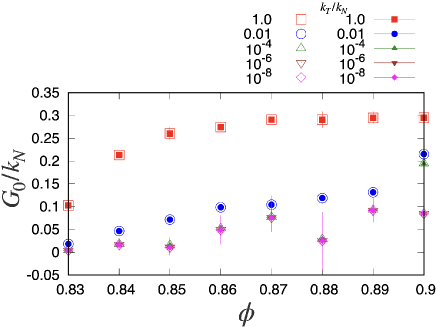
In this appendix, we verify the validity of our method to evaluate the rigidity G0G_{0} for frictional harmonic grains in the linear response regime for various kT/kNk_{T}/k_{N} and ϕ\phi as in Ref. Ishima2022 . Figure 16 presents the results of the rigidity, in which G0G_{0} obtained by the eigenvalue analysis (filled symbols) is in perfect agreement with that obtained by the simulation (open symbols). Here we take the average over 5 ensembles for each ϕ\phi and kTk_{T}. This figure confirms the validity of the theoretical method in the linear response regime.

Refer to caption
Figure 16: The plot of the rigidity G0G_{0} in the linear response regime for various kT/kNk_{T}/k_{N} and ϕ\phi, where open symbols and filled symbols are results of the theory and simulation, respectively.

References