EGSRAL:An Enhanced 3D Gaussian Splatting based Renderer with Automated Labeling for Large-Scale Driving Scene
Abstract
3D Gaussian Splatting (3D GS) has gained popularity due to its faster rendering speed and high-quality novel view synthesis. Some researchers have explored using 3D GS for reconstructing driving scenes. However, these methods often rely on various data types, such as depth maps, 3D boxes, and trajectories of moving objects. Additionally, the lack of annotations for synthesized images limits their direct application in downstream tasks. To address these issues, we propose EGSRAL, a 3D GS-based method that relies solely on training images without extra annotations. EGSRAL enhances 3D GS’s capability to model both dynamic objects and static backgrounds and introduces a novel adaptor for auto labeling, generating corresponding annotations based on existing annotations. We also propose a grouping strategy for vanilla 3D GS to address perspective issues in rendering large-scale, complex scenes. Our method achieves state-of-the-art performance on multiple datasets without any extra annotation. For example, the PSNR metric reaches 29.04 on the nuScenes dataset. Moreover, our automated labeling can significantly improve the performance of 2D/3D detection tasks. Code is available at https://github.com/jiangxb98/EGSRAL.
1 Introduction
Synthesizing novel photorealistic views represents a complex and crucial challenge in the fields of computer vision and graphics. With the rapid development of neural radiance fields (NeRFs) (Mildenhall et al. 2021), free-view synthesis has gradually transferred to the domain of large-scale view synthesis, particularly in synthesizing streetscapes critical for autonomous driving (Chen 2019). However, simulating outdoor environments is challenging due to the complexity of geographical locations, diverse surroundings, and varying road conditions. Image-to-image translation methods (Wang et al. 2018; Isola et al. 2017) have been proposed to synthesize semantically labeled streetscapes by learning the mapping between source and target images. While these methods generate visually impressive street views, they often exhibit noticeable artifacts and inconsistent textures in local details. Additionally, the relatively uniform viewpoints of the synthesized images present challenges for their application in complex autonomous driving scenes.
To address these challenges, Drive-3DAu (Tong et al. 2023) introduces a 3D data augmentation approach using NeRF, designed to augment driving scenes in the 3D space. DGNR (Li et al. 2023) presents a novel framework that learns a density space from scenes to guide the construction of a point-based renderer. Meanwhile, READ (Li, Li, and Zhu 2023) offers a large-scale driving simulation environment for generating realistic data for advanced driver assistance systems. 3D GS-based methods (Zhou et al. 2024; Yan et al. 2024) have been employed to synthesize driving scenes due to their superior generation capabilities. While these methods generate realistic images suitable for autonomous driving, they cannot simultaneously synthesize novel views and provide corresponding 2D/3D annotation boxes, which are crucial for supervised model training. Consequently, enhancing novel view synthesis for large-scale scenes and achieving automatic annotations for new views remain key challenges in autonomous driving.
To overcome these challenges, we introduce a novel framework called EGSRAL based on an enhanced 3D Gaussian Splatting (3D GS) technique. This framework improves the quality of novel view synthesis while simultaneously generating corresponding annotations. Specifically, we propose a deformation enhancement module to refine the Gaussian deformation field enhancing the modeling of both dynamic objects and static backgrounds. Additionally, we introduce an opacity enhancement module that leverages a neural network, replacing the original learnable parameter, to significantly boost the modeling capacity of complex driving scenes. Furthermore, to address the issue of unrealistic viewpoints in rendering large-scale complex scenes, where occluded distant Gaussians should not be included, we also propose a grouping strategy for vanilla 3D GS.
In short, our contributions are as follows: (1) We propose an enhanced 3D GS-based renderer called EGSRAL, which can synthesize novel view images with corresponding annotations based on existing dataset annotations. EGSRAL introduces a deformation enhancement module and an opacity enhancement module, both of which enhance the modeling capability of 3D GS for complex scenes. (2) Additionally, to address the issue of unreasonable perspectives in rendering large-scale, complex scenes, we introduce a grouping strategy for vanilla 3D GS. (3) Unlike previous methods that focus solely on novel view synthesis, we propose an adaptor with three constraints to transform neighboring annotation boxes into novel annotation boxes in the domain of autonomous driving. (4) Experimental results demonstrate that our method outperforms existing rendering methods for large-scale scenes. Additionally, the novel view images with corresponding annotations effectively improve the performance of 2D/3D detection models.
2 Related Work
2.1 3D Gaussian Splatting
Recently 3D GS has achieved exciting results in novel view synthesis and real-time rendering. Unlike NeRF, which uses implicit functions and volumetric rendering, 3D GS leverages a set of 3D Gaussians to model the scene, allowing for fast rendering through a tile-based rasterizer.
The original 3D GS (Kerbl et al. 2023) is designed to model static scenes, and subsequent work has tried to extend it to dynamic scenes. (Yang et al. 2024) introduce a deformation field to model monocular dynamic scenes, which use encoded Gaussian position and timestep to predict the position, rotation, and scaling offsets of 3D Gaussian. 4D GS (Wu et al. 2024) uses HexPlane (Cao and Johnson 2023) to encode temporal and spatial information for 3D Gaussian, building Gaussian features from 4D neural voxels, and then predicting the deformation of 3D Gaussians. However, compared to indoor scenes, outdoor scenes present greater challenges due to their larger spatial extent and the wider range of motion of dynamic objects. The above 3D GS methods often do not scale well to large-scale outdoor autonomous driving scenes. In contrast, our approach is more effective at reconstructing autonomous driving scenes.
2.2 Novel-View Synthesis for Driving Scene
Autonomous driving scene reconstruction methods based on NeRF can be roughly divided into two categories: perception-based (Fu et al. 2022; Xu et al. 2023; Kundu et al. 2022; Zhi et al. 2021) and simulation-based (Wu et al. 2023; Zhang et al. 2023; Li, Li, and Zhu 2023). Perception-based methods leverage capabilities of NeRF to capture the semantic information and geometrical representations. For simulation, MARS (Wu et al. 2023) models the foreground objects and background environments separately based on NeRF, making it flexible for scene controlling in autonomous driving simulation. Furthermore, READ (Li, Li, and Zhu 2023) explores diverse sampling strategies aimed at enabling the synthesis of expansive driving scenarios.
Some recent works have begun to bring 3D GS into the reconstruction of driving scenes. DrivingGaussian (Zhou et al. 2024) uses incremental static Gaussians and composite dynamic Gaussians to reconstruct static scenes and dynamic objects, respectively. Street Gaussians (Yan et al. 2024) represents the scene as a set of point-based background and foreground objects where an optimization strategy is introduced to deal with dynamic foreground vehicles. Although the above methods introduce a novel view synthesis paradigm into the autonomous driving domain, mainstream methods still heavily rely on annotated data. Simply synthesizing novel views without annotations can not be directly applied to the downstream perception tasks. Therefore, to address this challenge, we first propose a new framework for synthesizing new views based on the 3D GS while enabling automatic annotation of downstream perception tasks.

2.3 Auto Labeling With Scene Reconstruction
Currently, some works partially explored the potential of NeRFs to serve as data factories at a level to achieve auto labeling in other task domains (e.g., depth estimation (Chang et al. 2022), object detection (Ge et al. 2022), semantic segmentation (Zhi et al. 2021)) to further improve domain performance. For instance, NS (Tosi et al. 2023) introduces a NeRF-supervised training procedure which exploits rendered stereo triplets to compensate for occlusions and depth maps as proxy labels to improve the depth stereo performance. Semantic-NeRF (Zhi et al. 2021) extends NeRF to jointly encode semantics with appearance and geometry to complete and accurate 2D semantic labels which can be achieved using a small amount of in-place annotations specific to the scene. Neural-Sim (Ge et al. 2022) proposes a novel bilevel optimization algorithm to automatically optimize rendering parameters (pose, zoom, illumination) to generate optimal data for downstream tasks using NeRF, which substitutes the traditional graphics pipeline and synthesizes useful images. However, there is currently no work to introduce auto labeling into 3D GS scene reconstruction. Inspired by the above methods, we consider incorporating auto labeling in the autonomous driving domain to further advance downstream perception tasks.
3 Methodology
3.1 Overview
Given input image sequences of a driving scene and point clouds estimated through structure-from-motion (SfM) methods (Agisoft 2019; Schonberger and Frahm 2016), our EGSRAL framework can synthesize realistic driving scenes from multiple perspectives while automatically labeling the corresponding novel synthetic views. We also propose a grouping strategy to address perspective issues in large-scale driving scenes. Our framework is divided into two parts: an Enhanced 3D GS Rendering and a Novel View Auto Labeling, as illustrated in Figure 1. The 3D GS rendering is based on the Deformable 3D GS (Yang et al. 2024), which we have extended with innovative modules (Sec. 3.2) to improve novel view synthesis. For auto labeling, we introduce an adaptor to transform camera poses and bounding boxes, generating corresponding annotations for the novel views (Sec. 3.3).
3.2 Enhanced 3D GS Rendering
3D GS is typically used for modeling static scenes and its ability to handle dynamic scenes is limited. Recent research (Yang et al. 2024; Sun et al. 2024; Wu et al. 2024; Cao and Johnson 2023) has focused on improving dynamic scene modeling. We use Deformable 3D GS (Yang et al. 2024) as our baseline and apply it to automatic driving scene reconstruction. This approach employs a unified deformation field for both static backgrounds and dynamic objects. To better represent each Gaussian primitive’s state, we introduce a state attribute which implicitly indicates whether the primitive is static or dynamic. We further enhance the deformation field by incorporating a deformation enhancement module. This module decodes each Gaussian primitive’s state attribute and time encoding to determine the adjustment factor for the deformation field. Recognizing the importance of opacity in rendering, we also introduce an opacity enhancement module to improve the capacity.
Deformable 3D GS Network. To reduce data dependency, we use only image data for driving scene reconstruction. We begin by initializing a set of 3D Gaussians through SfM, where , , , and represent the position of the Gaussian primitive, quaternion, scaling, and opacity, respectively. To better model dynamic 3D Gaussians, the Deformable 3D GS introduces a deformation field for the 3D Gaussians. The deformation field takes the position and time as inputs to predict offsets , , and for , , and , respectively. Subsequently, these deformed 3D Gaussians are then passed through a differentiable tile rasterizer (Kerbl et al. 2023) to render the novel image:
| (1) |
where denotes the rendered color of the pixel, is the transmittance defined by , is the color of each Gaussian primitive, and is calculated by evaluating a 2D Gaussian with covariance matrix (Yifan et al. 2019) multiplied by a learned per-primitive opacity.
However, Deformable 3D GS struggles to effectively model dynamic objects and static backgrounds. We believe this limitation stems from the inability of 3D Gaussians to adequately represent both dynamic and static elements. To address this, we introduce a state attribute for each Gaussian primitive and incorporate it as an input to the deformable network. This enhancement improves the network’s ability to capture the state of the Gaussian primitives:
| (2) |
where represents the deformable network’s parameters, denotes a stop-gradient operation and is the positional encoding.
Deformation Enhancement Module (DEM). To further enhance the modeling of dynamic objects, we propose a deformation enhancement module that fine-tunes the deformation field based on the time and the state attribute of the Gaussian primitive. Specifically, we use the state attribute and time encoding as inputs to output an adjustment factor for each Gaussian primitive’s deformation field:
| (3) |
where represents the dynamic encoding network’s parameters, is the current camera’s coordinate position, and is the activation function.
Additionally, in driving scenes, we dynamically adjust the opacity of dynamic objects using an opacity adjustment factor to more effectively model their appearance and disappearance:
| (4) |
where is the activation function.
Using the adjustment factors and , we modify the attributes of deformed 3D Gaussians to , enabling the deformation field to model dynamic objects and static backgrounds with greater detail.
Opacity Enhancement Module (OEM). As seen in the image rendering formula (Equation 1), the rendering of the current pixel depends on the color and opacity of the Gaussian primitive. To enhance the capacity of opacity prediction, we initialize the Gaussian primitive by initializing opacity to a trainable parameter and introduce a lightweight network to accelerate opacity optimization:
| (5) |
where is the opacity enhancement module’s parameters.

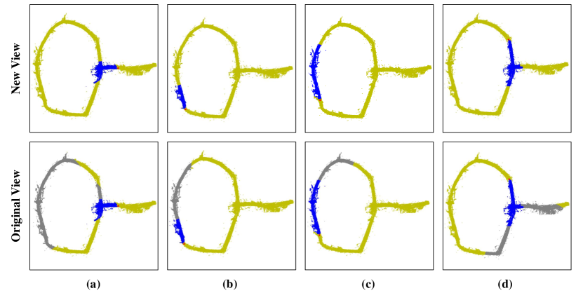
Grouping Strategy (GPS). Previous methods (Zhou et al. 2024; Yan et al. 2024) for reconstructing driving scenes using 3D GS have not accounted for large-scale scenes. To address this, we propose a grouping strategy. As illustrated in Figure 2(a), we divide the scene into groups using a fixed image interval and assign each Gaussian primitive a group identification , which allows us to perform subsequent cloning, splitting, and rendering based on these group s. By grouping strategy, we solve the problem of unreasonable fields of view. As shown in Figure 2(c), the original 3D GS rendering field of view includes distant Gaussian primitives (green rectangle), which is impractical. By grouping (red rectangle), we limit the field of view to a specific range, thus reducing the optimization burden by excluding Gaussian primitives outside this range.
Unlike the static incremental training mode in DrivingGaussian (Zhou et al. 2024), our method avoids sequential group training and the need for separate deformable networks for each group, leading to fewer models and shorter training times. However, the varying positional distribution of Gaussian primitives can affect convergence. To address this, we introduce a multi-group joint optimization strategy. As shown in Figure 2(b), each group performs forward propagation to accumulate gradients independently. After all groups have completed their forward passes, we perform gradient backpropagation to optimize the network parameters, stabilizing the training of the deformable network.
Additionally, to address the poor reconstruction quality of 3D GS in the initial frames, we propose an overlap training strategy. Specifically, for each group, we use images from the previous group to train the current group, significantly improving reconstruction quality. The detailed algorithm is provided in Appendix Algorithm 1.
3.3 Novel View Auto Labeling
Adaptor Requirement. Our method leverages image sequences (dataset) to construct scene point clouds and estimate camera poses and parameters using SfM methods. The generated point clouds and camera poses are defined in a new coordinate system generated by the SfM methods. However, the 3D annotations of the image sequences and corresponding camera poses are defined in the original world coordinate system, as in nuScenes (Caesar et al. 2020). Consequently, there exist two different coordinate systems: the original world coordinate system (OWCS) and the estimated world coordinate system (EWCS) from SfM methods.
Our renderer is trained based on the EWCS, as it takes the estimated points and camera poses in the EWCS as input. The novel camera poses used for generating novel view images are also based on the EWCS, which complicates the utilization of the dataset’s 3D annotations in the OWCS. A transformation adaptor is necessary to establish the relationship between the two coordinate systems, allowing us to utilize the 3D annotations effectively. This adaptor transforms coordinates from the OWCS to the EWCS. As a result, novel view camera poses from the OWCS can be converted into the EWCS and fed into the renderer to generate novel view images.
Our Adaptor. We take a neural network to model the transformation relationship of camera poses from the two coordinate systems, which takes camera poses in the OWCS as input and predicts the corresponding camera poses in the EWCS. We represent the camera pose as a 34 matrix that includes both rotation and translation information. Therefore the shapes of input and output are both 34. We take MLPs to build our adaptor, as shown in Figure 3, the backbone of our adaptor is composed of 8 layers of MLP, and the output head is a simple linear layer, which is used to predict camera poses in the EWCS. To optimize our adaptor, we introduce three constraints during the training process.

Constrains for Adaptor. To effectively train the adaptor, we need camera poses from the dataset in both coordinate systems. It is straightforward to obtain the existing camera pose pairs from these systems, where each pair consists of camera poses of the same frame from both the OWCS and the EWCS. We adopt the loss (Girshick 2015) to ensure that the adaptor’s predictions closely match the corresponding SfM camera poses in the EWCS, given the original camera poses in the OWCS. The loss function for camera pose constraints is:
| (6) |
where is the loss of the existing camera pose constraint, is the pose predicted by the adaptor given camera pose in the OWCS, and is the corresponding pose generated by SfM in the EWCS. After applying the initial constraint, the adaptor can transform existing camera poses between the two coordinate systems. However, due to the limited number of camera pose pairs, the adaptor’s generalization ability is restricted, resulting in poor performance with novel camera poses not included in the existing pairs. To address this issue, we introduce new camera pose constraints.
The novel camera pose constraints aim to enhance the adaptor’s generalization ability by utilizing existing data to constrain new camera poses. Based on the projection consistency rule of the same objects in two camera coordinate systems, we can construct projection constraints for new camera poses. Specifically, for a camera pose in the dataset, we use a Random Position Transformation (RPT) module to sample a nearby novel pose . This pose has a corresponding camera pose in the EWCS, which is implicit and not directly available. Next, we take the following camera pose pairs after the current camera pose and project them onto the corresponding novel camera pose planes in both coordinate systems. The corresponding projected points should have the same pixel coordinates. As shown in Figure 3, the coordinate conversion module (CCM) is used to convert points (the camera poses) in the OWCS to the camera coordinate system firstly by leveraging coordinate transformation formulas shown in Equation 7. In the coordinate system of the novel camera pose, the relative pose of is represented as .
| (7) |
where is the camera pose of the in the OWCS, is the novel camera pose, sampled nearby the current frame in the OWCS. Then, we project these points to the novel camera pose plane. As shown in Figure 3, the point project module (PPM) is used to project points from the camera coordinate system to the pixel coordinate system. Next, we calculate the coordinate of in the pixel coordinate system of the novel camera pose plane by utilizing the camera intrinsic parameters, as illustrated in Equation 8 and 9 below:
| (8) | ||||
| (9) |
where is camera intrinsic parameter matrix, and is the translation of . Then the projection constraint can be summarized as shown in Equation 10.
| (10) |
where is the pixel coordinate of the relative camera pose in the EWCS projected to the novel camera pose plane. is predicted by our adaptor fed with novel camera pose as shown in Figure 3. Our adaptor aims to ensure that is equal to by making equal to . is estimated by using the projected pixel coordinates from the corresponding camera poses in the OWCS as shown in Figure 3 based on the projection consistency rule.
Due to the limitations of pixel coordinate constraints (as in Equation 10), which only restrict the relationship between and and between and without determining their specific values, the adaptor fails to converge to the desired outcome. Including the constraints on the position in the camera coordinate system (as in Equation 11) into effectively resolves the aforementioned issue. Given the similarity between real camera intrinsic parameters and those estimated by SfM, it is possible to assume identical position information in the camera coordinate system during the initial stages of adaptor training. Subsequently, the weight on the camera coordinate system constraints can be appropriately reduced. The overall loss is expressed as in Equation 12 below:
| (11) | ||||
| (12) |
where is the 3D coordinate of the relative camera pose of camera pose in the EWCS relative to novel camera pose , as shown in Figure 3. is the estimated 3D coordinate of the relative camera pose of the camera pose in the EWCS, relative to novel camera pose , obtained using the 3D coordinates from the corresponding camera poses in the OWCS. is the loss of novel camera pose constraints in 3D coordinates, is the loss of novel camera pose constraints in project pixel coordinates, is the weight of , is the weight of , is the weight of .
Annotation Generation. During the inference phase, as illustrated in Figure 1, we start with the original camera pose in the OWCS from the dataset. This pose undergoes an affine random transformation to obtain by the RPT module shown in Figure 3. Then we feed into the adaptor to produce the corresponding pose in the EWCS, denoted as . Feeding into the renderer generates the corresponding novel view image, called . Similarly, applying the same affine transformation to the original dataset’s annotations results in , which corresponds to . Combining with results in a novel view image with annotations, effectively accomplishing auto labeling.
4 Experiment
4.1 Datasets
KITTI Dataset. KITTI dataset (Geiger, Lenz, and Urtasun 2012) contains a wide range of driving scenes. Our experiments focus on a single distinct scene: City, which consists of 1424 train images and 159 test images.
4.2 Experimental Settings
Implementation Details. Our implementation is primarily based on Deformable 3D GS (Yang et al. 2024), maintaining consistency with its training iterations and optimizer settings. Additionally, the DEM and the OEM are optimized using Adam with a learning rate of 0.001.
Adaptor Model Training Settings. Our training dataset is nuScenes poses and poses generated by SfM as data pairs. We need to train on 17 different scenes, each with approximately 230 pose pairs. Each scene requires training for 1000 epochs. We use the Adam optimizer with a learning rate of 2e-4 and a batch size of 16. It takes about 2 hours to train using AMD MI100. Adaptor model loss weights , and in Equation 12 are 50, 0.1 and 1, respectively, and the camera pose is 15.
2D/3D Detection Settings. To verify the effectiveness of synthetic data, we use mainstream detection model to perform 2D and 3D detection tasks on four categories: car, bus, truck, and trailer. 2D detection tasks use Co-DETR (Zong, Song, and Liu 2023a) and 3D tasks use MonoLSS (Li, Jia, and Shi 2024). For the test dataset, we select the first fifteen scene data in the nuScenes validation set.
Methods Supervision PSNR LPIPS SSIM NPBG RGB + Points 19.58 0.248 0.628 ADOP RGB + Points 20.08 0.183 0.623 Deepview RGB 17.28 0.196 0.716 MPI RGB 19.54 0.158 0.733 READ RGB 23.48 0.132 0.787 3D GS RGB 20.37 0.357 0.679 Mip-splatting RGB 20.86 0.341 0.696 Deformable 3D GS RGB 21.33 0.306 0.713 EGSRAL(Ours) RGB 23.60 0.192 0.787
Methods Input PSNR LPIPS SSIM S-NeRF RGB+LiDAR 25.43 0.302 0.730 SUDS RGB+LiDAR 21.26 0.466 0.603 EmerNeRF RGB+LiDAR 26.75 0.311 0.760 3D GS RGB+SfM 26.08 0.298 0.717 DrivingGaussian-L RGB+LiDAR 28.74 0.237 0.865 EGSRAL(Ours) RGB+LiDAR 29.04 0.162 0.883
4.3 Performance of Novel View Synthesis
Evaluation on KITTI. We compare our method with state-of-the-art (SOTA) methods, as shown in Table 1. Our approach demonstrates superior performance compared to other 3D GS methods, with PSNR and SSIM improvements of 2.27 and 0.074, respectively, and 0.114 reduction in LPIPS over Deformable 3D GS. Additionally, compared to other methods like READ, our method enhances the PSNR metric to 23.60 while achieving comparable SSIM results. However, the 3D GS-based method has a slight deficiency in modeling high-frequency information, such as ground texture, which leads to a higher LPIPS. For detailed visualization results, please refer to the supplementary materials.
Methods PSNR LPIPS SSIM Mip-NeRF 18.22 0.421 0.655 Mip-NeRF360 24.37 0.240 0.795 Urban-NeRF 21.49 0.491 0.661 S-NeRF 26.21 0.228 0.831 3D GS 32.82 0.225 0.925 Mip-splatting 32.22 0.224 0.928 Deformable 3D GS 33.43 0.224 0.932 EGSRAL(Ours) 34.43 0.205 0.939

Evaluation on nuScenes. Following the scenes used by DrivingGaussian, as shown in Table 2, our method achieves the highest performance, with an increase of 0.3 and 0.018 in PSNR and SSIM, respectively, and a decrease of 0.075 in the LPIPS. It is worth noting that DrivingGaussian trains the dynamic objects and the static backgrounds separately, training an individual 3D GS model for each dynamic object then merging them. In contrast, our method requires only a single training process and does not need any annotations, resulting in better performance and reducing the dependence on data annotations.
Following the scenes used by S-NeRf (Xie et al. 2023), as shown in Table 3, we contrast our method with the SOTA method. In addition, we replicated 3D GS (Kerbl et al. 2023), Deformable 3D GS (Yang et al. 2024), and mip-splatting (Yu et al. 2024) on this dataset. The 3D GS-based method has much higher metrics on these scenes than the NeRf-based method. Our method achieves the best performance, with PSNR improved by 1.00, SSIM improved by 0.007, and LPIPS reduced by 0.019 compared to the Deformable 3D GS.
In Figure 4, we compare the view synthesis results of our method with those of other 3D GS methods. The visualization results show superior synthesis capabilities, especially achieving more realistic rendering results on static backgrounds (trees) and dynamic objects (pedestrians).
4.4 Performance of Auto Labeling
We select 17 different scenes from the nuScenes dataset for the 2D/3D auto-labeling task. Using the adaptor, we generate novel view images and automatically label them simultaneously. The results are presented in Figure 5. The three columns represent three different scenes: the first row displays the original images, while the last two rows show the novel view images with auto labeling. In these images, the yellow boxes denote 2D annotations, and the orange boxes denote 3D annotations. The results demonstrate that our adaptor performs effectively across different scenes.
Performance of 2D/3D Object Detection. We select 17 different scenes containing 3,898 images (674 of which are sample images with annotations) from the nuScenes dataset as the baseline dataset for the detection task. We produce the annotations for the non-sample images based on the annotations of sample images by camera coordinate system transformation. To augment the dataset, we synthesize additional images using an adaptor, increasing the total number of images to two and three times that of the baseline dataset. The 2D detection results are presented in Table 4, and the 3D detection results are presented in Table 5. In these tables, refers to the 674 sample images, while refers to the 3,898 images, including both sample and non-sample images. The results demonstrate that, without any additional input, our data augmentation method improves the accuracy of the detection model in both the and the dataset.
Model Dataset Total_amount mAP AP50 AP75 Co-DETR sample 1 23.7 44.6 22.9 2 25.9 45.9 23.1 3 26.8 46.1 23.2 all 1 28.1 46.5 24.2 2 29.9 47.7 24.8 3 31.3 48.2 25.3
Model Dataset Total_amount AP3d Mod. Hard MonoLSS sample 1 17.21 12.55 11.30 2 19.78 13.32 12.81 3 20.31 13.85 12.97 all 1 21.69 14.27 13.95 2 22.15 14.93 14.22 3 22.87 15.25 14.40

4.5 Ablation Study and Analysis
In this section, we provide ablation experiments for different modules of our method on the KITTI City dataset, as shown in Table 6. For more experiments and analyses, please see Appendix Section 3. Comparing rows 2 and 3, we observe that using the DEM alone to refine the deformation field improves PSNR by 1.04 and SSIM by 0.03. In contrast, using the OEM alone results in improvements of 0.99 in PSNR and 0.025 in SSIM, with a reduction of 0.029 in LPIPS. When both DEM and OEM are combined, the evaluation metrics show significant improvements over Deformable 3D GS, demonstrating the enhanced synthesis capabilities of our method for large-scale scene modeling. Additionally, we validate our proposed grouping strategy. As shown in the last row, our approach further enhances PSNR by 0.76, improves SSIM by 0.027, and reduces LPIPS by 0.061 by incorporating the grouping strategy. In conclusion, the above ablation studies fully validate the effectiveness of all proposed modules in our method.
DEM OEM GPS PSNR LPIPS SSIM - - - 21.33 0.306 0.713 - - 22.37 0.279 0.743 - - 22.32 0.277 0.738 - 22.84 0.253 0.760 23.60 0.192 0.787
5 Conclusion
In this paper, we present EGSRAL, a novel 3D GS-based renderer with an automated labeling framework capable of synthesizing novel view images with corresponding annotations. For novel view rendering, we introduce two effective modules to improve the ability of 3D GS to model complex scenes and propose a grouping strategy to solve the problem of unreasonable view of large-scale scenes. For novel view auto labeling, we propose an adaptor to generate new annotations for novel views. Experimental results show that EGSRAL significantly outperforms existing methods in novel view synthesis and achieves superior object detection performance on annotated images.
References
- Agisoft (2019) Agisoft. 2019. Agisoft: Metashape software]. retrieved 20.05.2019 (2019).
- Caesar et al. (2020) Caesar, H.; Bankiti, V.; Lang, A. H.; Vora, S.; Liong, V. E.; Xu, Q.; Krishnan, A.; Pan, Y.; Baldan, G.; and Beijbom, O. 2020. nuscenes: A multimodal dataset for autonomous driving. In CVPR, 11621–11631.
- Cao and Johnson (2023) Cao, A.; and Johnson, J. 2023. Hexplane: A fast representation for dynamic scenes. In CVPR, 130–141.
- Chang et al. (2022) Chang, D.; Božič, A.; Zhang, T.; Yan, Q.; Chen, Y.; Süsstrunk, S.; and Nießner, M. 2022. RC-MVSNet: unsupervised multi-view stereo with neural rendering. In ECCV, 665–680. Springer.
- Chen (2019) Chen, S.-C. 2019. Multimedia for autonomous driving. IEEE MultiMedia, 5–8.
- Fu et al. (2022) Fu, X.; Zhang, S.; Chen, T.; Lu, Y.; Zhu, L.; Zhou, X.; Geiger, A.; and Liao, Y. 2022. Panoptic nerf: 3d-to-2d label transfer for panoptic urban scene segmentation. In 3DV, 1–11. IEEE.
- Ge et al. (2022) Ge, Y.; Behl, H.; Xu, J.; Gunasekar, S.; Joshi, N.; Song, Y.; Wang, X.; Itti, L.; and Vineet, V. 2022. Neural-sim: Learning to generate training data with nerf. In ECCV, 477–493. Springer.
- Geiger, Lenz, and Urtasun (2012) Geiger, A.; Lenz, P.; and Urtasun, R. 2012. Are we ready for autonomous driving? the kitti vision benchmark suite. In CVPR, 3354–3361. IEEE.
- Girshick (2015) Girshick, R. 2015. Fast r-cnn. In ICCV, 1440–1448.
- Isola et al. (2017) Isola, P.; Zhu, J.-Y.; Zhou, T.; and Efros, A. A. 2017. Image-to-image translation with conditional adversarial networks. In CVPR, 1125–1134.
- Kerbl et al. (2023) Kerbl, B.; Kopanas, G.; Leimkühler, T.; and Drettakis, G. 2023. 3D Gaussian Splatting for Real-Time Radiance Field Rendering. ACM Trans. Graph., 139–1.
- Kundu et al. (2022) Kundu, A.; Genova, K.; Yin, X.; Fathi, A.; Pantofaru, C.; Guibas, L. J.; Tagliasacchi, A.; Dellaert, F.; and Funkhouser, T. 2022. Panoptic neural fields: A semantic object-aware neural scene representation. In CVPR, 12871–12881.
- Li, Jia, and Shi (2024) Li, Z.; Jia, J.; and Shi, Y. 2024. MonoLSS: Learnable Sample Selection For Monocular 3D Detection. In 3DV, 1125–1135. IEEE.
- Li, Li, and Zhu (2023) Li, Z.; Li, L.; and Zhu, J. 2023. Read: Large-scale neural scene rendering for autonomous driving. In AAAI, 1522–1529.
- Li et al. (2023) Li, Z.; Wu, C.; Zhang, L.; and Zhu, J. 2023. DGNR: Density-Guided Neural Point Rendering of Large Driving Scenes.
- Mildenhall et al. (2021) Mildenhall, B.; Srinivasan, P. P.; Tancik, M.; Barron, J. T.; Ramamoorthi, R.; and Ng, R. 2021. Nerf: Representing scenes as neural radiance fields for view synthesis. Communications of the ACM, 99–106.
- Schonberger and Frahm (2016) Schonberger, J. L.; and Frahm, J.-M. 2016. Structure-from-motion revisited. In CVPR, 4104–4113.
- Sun et al. (2024) Sun, J.; Jiao, H.; Li, G.; Zhang, Z.; Zhao, L.; and Xing, W. 2024. 3dgstream: On-the-fly training of 3d gaussians for efficient streaming of photo-realistic free-viewpoint videos. In CVPR, 20675–20685.
- Tong et al. (2023) Tong, W.; Xie, J.; Li, T.; Deng, H.; Geng, X.; Zhou, R.; Yang, D.; Dai, B.; Lu, L.; and Li, H. 2023. 3D Data Augmentation for Driving Scenes on Camera.
- Tosi et al. (2023) Tosi, F.; Tonioni, A.; De Gregorio, D.; and Poggi, M. 2023. NeRF-Supervised Deep Stereo. In CVPR, 855–866.
- Umeyama (1991) Umeyama, S. 1991. Least-squares estimation of transformation parameters between two point patterns. IEEE Transactions on Pattern Analysis & Machine Intelligence, 376–380.
- Wang et al. (2018) Wang, T.-C.; Liu, M.-Y.; Zhu, J.-Y.; Tao, A.; Kautz, J.; and Catanzaro, B. 2018. High-resolution image synthesis and semantic manipulation with conditional gans. In CVPR, 8798–8807.
- Wu et al. (2024) Wu, G.; Yi, T.; Fang, J.; Xie, L.; Zhang, X.; Wei, W.; Liu, W.; Tian, Q.; and Wang, X. 2024. 4d gaussian splatting for real-time dynamic scene rendering. In CVPR, 20310–20320.
- Wu et al. (2023) Wu, Z.; Liu, T.; Luo, L.; Zhong, Z.; Chen, J.; Xiao, H.; Hou, C.; Lou, H.; Chen, Y.; Yang, R.; et al. 2023. Mars: An instance-aware, modular and realistic simulator for autonomous driving.
- Xie et al. (2023) Xie, Z.; Zhang, J.; Li, W.; Zhang, F.; and Zhang, L. 2023. S-nerf: Neural radiance fields for street views.
- Xu et al. (2023) Xu, C.; Wu, B.; Hou, J.; Tsai, S.; Li, R.; Wang, J.; Zhan, W.; He, Z.; Vajda, P.; Keutzer, K.; et al. 2023. Nerf-det: Learning geometry-aware volumetric representation for multi-view 3d object detection. In ICCV, 23320–23330.
- Yan et al. (2024) Yan, Y.; Lin, H.; Zhou, C.; Wang, W.; Sun, H.; Zhan, K.; Lang, X.; Zhou, X.; and Peng, S. 2024. Street gaussians for modeling dynamic urban scenes.
- Yang et al. (2024) Yang, Z.; Gao, X.; Zhou, W.; Jiao, S.; Zhang, Y.; and Jin, X. 2024. Deformable 3d gaussians for high-fidelity monocular dynamic scene reconstruction. In CVPR, 20331–20341.
- Yifan et al. (2019) Yifan, W.; Serena, F.; Wu, S.; Öztireli, C.; and Sorkine-Hornung, O. 2019. Differentiable surface splatting for point-based geometry processing. TOG, 1–14.
- Yu et al. (2024) Yu, Z.; Chen, A.; Huang, B.; Sattler, T.; and Geiger, A. 2024. Mip-Splatting: Alias-free 3D Gaussian Splatting. In CVPR, 19447–19456.
- Zhang et al. (2023) Zhang, J.; Zhang, F.; Kuang, S.; and Zhang, L. 2023. NeRF-LiDAR: Generating Realistic LiDAR Point Clouds with Neural Radiance Fields.
- Zhi et al. (2021) Zhi, S.; Laidlow, T.; Leutenegger, S.; and Davison, A. J. 2021. In-place scene labelling and understanding with implicit scene representation. In ICCV, 15838–15847.
- Zhou et al. (2024) Zhou, X.; Lin, Z.; Shan, X.; Wang, Y.; Sun, D.; and Yang, M.-H. 2024. Drivinggaussian: Composite gaussian splatting for surrounding dynamic autonomous driving scenes. In CVPR, 21634–21643.
- Zong, Song, and Liu (2023a) Zong, Z.; Song, G.; and Liu, Y. 2023a. DETRs with Collaborative Hybrid Assignments Training. In ICCV, 6748–6758.
- Zong, Song, and Liu (2023b) Zong, Z.; Song, G.; and Liu, Y. 2023b. Detrs with collaborative hybrid assignments training. In Proceedings of the IEEE/CVF international conference on computer vision, 6748–6758.
6 Appendix
In this supplementary material, we present more implementation details and additional experimental results.
-
•
In Section 7, we present the training details of our method, the specific implementation of the grouping strategy algorithm, and the performance comparison of the latest 2D and 3D detectors.
-
•
In Section 8, we present additional experimental results.
-
•
In Section 9, we present the KITTI dataset visualization results and more adaptor visualization results.
7 Implementation Details
7.1 Experiment Setting
KITTI Selected by READ. For the KITTI dataset, we follow the setup of READ (Li, Li, and Zhu 2023) and use the single camera as input, with a resolution of . We select every 10th image of cameras in the sequences as the test set. See Table 7 for the detailed hyperparameter settings.
NuScenes-S Selected by S-NeRF. For the NuScenes-S dataset, we follow the setup of S-NeRF (Xie et al. 2023) and only use the front camera as input, with a resolution of . We select every 4th image of cameras in the sequences as the test set. The specific scene tokens are 164, 209, 359, and 916. We report the average results of all camera frames on the selected scenes and assess our models using the average score of PSNR, SSIM, and LPIPS. See Table 7 for the detailed hyperparameter settings.
NuScenes-D Selected by DrivingGaussian.
Hyperparameter 3DGS Mip-Splatting D3DGS EGSRAL (Ours) KITTI nuScenes-S KITTI nuScenes-S KITTI nuScenes-S KITTI nuScenes-S nuScenes-D Training iterations 2,000,000 40,000 2,000,000 40,000 2,000,000 40,000 40,000 40,000 200,000 Warm up iteration - - - - 90,000 3,000 3,000 3,000 30,000 Densification interval 3,000 100 3,000 100 3,000 100 100 100 300 Opacity reset interval 90,000 3,000 90,000 3,000 90,000 3,000 3,000 3,000 6,000 Densify from iteration 15,000 500 15,000 500 15,000 500 500 500 5,000 Densify until iteration 500,000 15,000 500,000 15,000 500,000 15,000 15,000 15,000 100,000 Densify grad threshold 0.0002 0.0002 0.0002 0.0002 0.0002 0.0002 0.0002 0.0002 0.0001
For the NuScenes-D dataset, we follow the setup of DrivingGaussian (Zhou et al. 2024) and use synchronized images from 6 cameras in surrounding views as inputs, with a resolution of . We select every 5th image of cameras in the sequences as the test set. The specific scene tokens are 103, 168, 212, 220, 228, and 687. We report the average results of all camera frames on the selected scenes and assess our models using the average score of PSNR, SSIM, and LPIPS. See Table 7 for the detailed hyperparameter settings.
To compare with DrivingGaussian, we utilize LiDAR point clouds to initialize the 3D Gaussians. Specifically, we stack the LiDAR point clouds of the entire scene and retrieve the corresponding image color of each point through the projection relationship. Finally, the voxelized downsampled point cloud is used to initialize the 3D Gaussians.
7.2 The Detailed Grouping Strategy
We propose the grouping strategy for the large-scale driving scene reconstruction. While DrivingGaussian (Zhou et al. 2024) also mentions incremental training, this is for the small nuScenes scene and does not carefully consider how to apply it to large-scale driving scenes like KITTI. Table 8 shows the difference between our method and DrivingGaussian, although both of them group the scene point cloud, DrivingGaussian is static incremental training, which needs to be trained in the order of the groups. On the contrary, our method only needs to assign a group to each Gaussian primitive, and the training process is shuffled. In addition, the DrivingGaussian method needs to train a model for each dynamic object and grouping scene during training. This approach not only depends on additional annotations but also necessitates the training of multiple models. In contrast, our method eliminates the need for extra annotations and requires training only a single model.
Algorithm 1 presents the detailed pseudocode implementation, while Figure 6 provides additional visualizations of the grouping strategy. By utilizing this strategy, we not only achieve more efficient reconstruction of large-scale driving scenes but also address issues related to unreasonable fields of view.
DrivingGaussian EGSRAL(Ours) Group Training mode Order Shuffle Network Number 1
Detector Year Backbone AP MS-DETR CVPR 2024 R50 51.7 RT-DETR CVPR 2024 R50 53.1 Co-DETR ICCV 2023 R50 54.8 DINO ICLR 2023 R50 49.4 Group DETR ICCV 2023 R50 50.1
7.3 SOTA 2D/3D Detector
2D Detector. We survey recent works on 2D detection, as shown in Table 9. Co-DETR (Zong, Song, and Liu 2023b) achieves high AP on the COCO validation set, demonstrating strong competitiveness compared to several current mainstream methods. This performance positions it as a SOTA model in object detection.
3D Detector. MonoLss (Li, Jia, and Shi 2024) achieves state-of-the-art performance in the primary categories of car, cyclist, and pedestrian on the KITTI monocular 3D object detection benchmark, as shown in Table 10. It also demonstrates strong competitiveness in cross-dataset evaluations on the Waymo, KITTI, and nuScenes datasets. At the time of our experiments, MonoLss is the leading open-source 3D detection model that relies solely on monocular image input.
Detector Year AP_BEV (IoU=0.7|R40) Easy Mod. Hard MonoLss 3DV 2024 34.89 25.95 22.59 DEVIANT ECCV 2022 29.65 20.44 17.43 MonoCon AAAI 2022 31.12 22.10 19.00 MonoDDE CVPR 2022 33.58 23.46 20.37
Method 164 209 359 916 Average PSNR SSIM LPIPS PSNR SSIM LPIPS PSNR SSIM LPIPS PSNR SSIM LPIPS PSNR SSIM LPIPS 3DGS 35.45 0.942 0.209 33.71 0.950 0.248 30.78 0.903 0.240 31.32 0.926 0.201 32.82 0.925 0.225 Mip-Splatting 34.28 0.935 0.213 32.84 0.944 0.252 30.41 0.901 0.238 31.34 0.931 0.191 32.22 0.928 0.224 Deformable 3D GS 35.87 0.943 0.208 35.37 0.956 0.241 30.48 0.898 0.246 32.00 0.930 0.199 33.43 0.932 0.224 EGSRAL(Ours) 36.32 0.946 0.193 36.48 0.963 0.216 31.94 0.911 0.218 32.99 0.936 0.191 34.43 0.939 0.205
Method Metric 103 168 212 220 228 687 Avg. EGSRAL(Ours) PSNR 28.87 28.52 30.10 28.87 29.36 28.48 29.04 SSIM 0.874 0.884 0.905 0.863 0.889 0.885 0.883 LPIPS 0.170 0.168 0.141 0.178 0.159 0.153 0.162 DrivingGaussian PSNR - - - - - - 28.74 SSIM - - - - - - 0.865 LPIPS - - - - - - 0.237
8 Additional Experiments
8.1 Detailed Results on nuScenes
8.2 Ablation Study
Effect of the Group Number in GPS. In Table 13, we present the results of our grouping strategy under different numbers of groups. With a small number of groups, the large scene leads to an unreasonable field of view after grouping, preventing effective training for each group. Conversely, with too many groups, the correct field of view is restricted, increasing the optimization burden of 3D GS. Ultimately, we achieve the best performance with 8 groups.
Group 4 6 8 10 PSNR 22.64 23.10 23.60 23.38
Effect of the Number of Camera Poses. For the adaptor, we conduct an ablation study on the number of camera poses, as shown in Table 14. During the adaptor’s training process, the number of camera poses is set to 15. By comparing the 2nd, 3rd, and 4th rows, it is evident that, compared to using 10 or 20 camera poses, selecting 15 has improved the accuracy of 3D frame alignment in novel-view images, enhancing the performance of the 3D detection task.
Model AP3D Mod. Hard MonoLSS - 17.21 12.55 11.30 10 18.55 12.87 12.11 15 19.78 13.32 12.81 20 19.67 13.26 12.73
8.3 Necessity Analysis of Adaptor
To address the complex alignment errors among camera poses in OWCS and EWCS, we propose a trainable adaptor with sampling pose augmentation, replacing the traditional transformation matrix estimation using the Umeyama algorithm (Umeyama 1991). The SfM method used in 3D GS is monocular, which limits its ability to produce high-quality reconstructions across diverse scenes. This limitation often results in the introduction of outliers, such as matching errors within the SfM process, leading to inconsistent alignment. These challenges make it difficult for traditional methods to achieve reliable results in such scenarios.
Metric Matrix Adaptor AP (%) 21.71 72.53 AD () 1.867 0.605

To evaluate their accuracy, we conduct experiments on the nuScenes-655 scene, reserving one-fourth of the data as a test set and using the remaining data to optimize both methods. During testing, the camera poses in EWCS are first transformed into corresponding poses in OWCS via both methods. Then the fixed 3D positions of objects in the vehicle coordinate system are transformed into global 3D positions in OWCS based on the generated camera poses of both methods, and the new 3D annotation positions in OWCS of each transformation method can be obtained. We calculate the AP and average 3D center distance between the GT 3D boxes and the generated 3D boxes in OWCS, as shown in Table 15. Our method significantly outperforms the standard matrix transformation-based method in both AP and average distance (AD) metrics, highlighting the advantages of our adaptor. Additionally, the visualization results in Figure 7 further demonstrate the superiority of our method.
To verify the robustness of the Adaptor’s data augmentation method, we expanded the original 2D/3D object detection dataset by doubling its size—from 17 scenes containing 3,898 images (674 of which are annotated sample images) to 34 scenes containing 8,497 images (1,455 of which are annotated sample images). As shown in Tables 16 and 17, the Adaptor’s data augmentation method consistently demonstrates significant improvements in the accuracy of 2D/3D object detection.
Model Dataset Total_amount mAP AP50 AP75 Co-DETR sample 1 28.6 47.1 24.5 2 30.2 47.8 25.1 3 31.5 48.4 25.4 all 1 32.4 49.0 25.8 2 33.2 49.5 25.9 3 33.7 49.7 26.2
Model Dataset Total_amount AP3d Mod. Hard MonoLSS sample 1 22.16 14.89 14.10 2 23.36 15.36 14.55 3 23.89 15.61 14.86 all 1 24.26 15.83 15.02 2 24.73 16.05 15.19 3 24.95 16.19 15.25
8.4 Complexity and Limitations

Complexity. Our rendering model builds upon and improves Deformable 3D GS. To demonstrate the effectiveness of our approach, we compare the average rendering speed between Deformable 3D GS and our method on a reconstructed KITTI scene. Specifically, on an NVIDIA V100 with approximately 4 million Gaussian primitives, Deformable 3D GS requires 0.768s to render a single frame, whereas our method (with 8 groups) only takes 0.254s. By applying our grouping strategy to Deformable 3D GS, the rendering speed is further improved to 0.199s. These results highlight that, despite the additional computational complexity introduced by our two enhancement modules, our method still achieves superior rendering speed compared to Deformable 3D GS. This improvement is primarily attributed to our novel grouping strategy, which efficiently groups Gaussian primitives and mitigates issues related to an excessive field of view. As a result, the number of Gaussian primitives required for rendering is reduced, significantly accelerating the overall rendering process.
Limitations. Since our rendering method is based on the 3D GS framework, it inherits the limitations of this approach. The 3D GS process begins by initializing the attributes of the 3D GS primitives—such as center position, opacity, and 3D covariance matrix—using point clouds generated by the SfM method. This is followed by an optimization and training phase. Consequently, the quality of the reconstruction depends on the accuracy of the point clouds produced by the SfM method.
9 Visualization
9.1 Visualization on KITTI.
Figure 8 shows the rendering results of the 3D GS-based method. It can be easily seen that our method obtains the best rendering quality among the 3D GS-based methods. However, a closer inspection shows that the 3D GS-based method cannot render the high-frequency information of the ground texture normally, which is also an important reason for its low LPIPS metric.
9.2 More Adaptor Auto Labeling Result.
We provide more qualitative results of auto labeling via our adaptor. The 3D results are presented in Figure 9, and the 2D results are shown in Figure 10. The three columns represent three different scenes. The first row displays the original images and their annotations, indicated by a green frame, while the last two rows show the novel view images with auto-labeling generated by the adaptor. The results demonstrate that our adaptor performs effectively across different scenes in both 2D and 3D annotations.

