Efficient simulation of mixed boundary value problems and conformal mappings

Recall that the modulus of a quadrilateral $Q$ is closely related to a the Dirichlet–Neumann mixed boundary value problem(Dirichlet–Neumann problem, in short) of Laplace equation, see e.g. [18, p. 431].

For quadrilateral $Q=(\Omega;z_{1},z_{2},z_{3},z_{4})$, we consider the boundary segments $\gamma_{j}$, for $j=1,2,3,4$, as the parts of $\partial\Omega$ connecting $z_{1}$ to $z_{2}$, $z_{2}$ to $z_{3}$, $z_{3}$ to $z_{4}$, and $z_{4}$ back to $z_{1}$, respectively. Let $\Gamma_{D}=\gamma_{2}\cup\gamma_{4}$, $\Gamma_{N}=\gamma_{1}\cup\gamma_{3}$ and $u$ be the (unique) harmonic solution to the Dirichlet–Neumann mixed boundary value problem:

Then by Ahlfors [2, Theorem 4.5] and Papamichael and Stylianopoulos [31, Theorem 2.3.3])

The problem for the conjugate quadrilateral $\widetilde{Q}$ is called the conjugate Dirichlet–Neumann problem.

1. (1)

   Find the solution $u$ to the Dirichlet–Neumann problem (3).

2. (2)

   Find the solution $\tilde{u}$ to the Dirichlet–Neumann problem associated with $\widetilde{Q}$.

3. (3)

   Pick a suitable point inside the domain (usually near the center of the domain) and evaluate suitable pairs of partial derivatives $\{u_{x},\tilde{u}_{y}\}$ and $\{\tilde{u}_{x},u_{y}\}$, where $z=x+iy$. If $f=u+ih\tilde{u}$ is a conformal mapping, it satisfies the Cauchy–Riemann equations. Therefore we can compute $h$ as

   $$h=\frac{u_{x}}{\tilde{u}_{y}}\text{ or }h=-\frac{u_{y}}{\tilde{u}_{x}}$$

   The vertices $\{z_{1},z_{2},z_{3},z_{4}\}$ are mapped onto the corners $\{1+ih,ih,0,1\}$.

The partial derivatives of $u$ and $\tilde{u}$ can be estimated using the five-point formula [1, p. 883] :

The error term for this approximation depends on the fourth derivative of $u(x,y)$ and is given by:

where $\xi$ is a point in the interval $[x-2\Delta x,x+2\Delta x]$.

It is clear that solving the Dirichlet–Neumann problem (3) is the key step. Section 4 will introduce a stochastic approach to solve it numerically through simulation, which we call the Reflected Walk-on-Spheres (RWoS) method.

Recall the following definition of the harmonic measure. For details we refer to [10, Chapter I].

Brownian motion in the plane, or the complex Brownian motion, exhibits a conformal invariance, see e.g. [23, Theorem 2.2]. Indeed, let $f$ be a conformal mapping from domain $\Omega$ onto $\Omega^{\prime}$. If $B$ is a complex Brownian motion on $\Omega$ then $f(B)$ admits the representation

where $\widetilde{B}$ is another complex Brownian motion. Thus the image trajectory of a Brownian motion under conformal mapping is still a trajectory of Brownian motion.

Thus if we choose the conformal mapping $\phi$ from $\Omega$ to $\mathbb{D}$ such that $\phi(z_{0})=0$, when a Brownian particle starting at that point $z_{0}$ in $\Omega$ exits the domain through $E$, we would observe in $\mathbb{D}$ that the Brownian particle starting at 0 and exits the domain through $\phi^{-1}(E)$. So we can conclude the probability of $z$ hitting $E$ is precisely the harmonic measure $\omega(z,E,\Omega)=|\phi^{-1}(E)|$. More generally speaking, the probability of the Brownian motion hitting a particular part of the boundary in the conformally transformed domain is the same as in the original domain [23].

The next definition introduces a powerful function for dealing with reflection at Neumann boundaries in RWoS algorithm.

The reversal of orientation in anti-conformal mappings changes the trajectories of the Brownian paths by mirroring them. Consequently, a Brownian trajectory remains a Brownian trajectory under anti-conformal maps.

The connection between Dirichlet boundary value problems and Brownian motion is due to Kakutani in 1944 [19]. Kakutani showed that the solution to the Dirichlet problem can be represented in terms of Brownian motion. Specifically, if a Brownian motion starts from a point inside $\Omega$, the value of the harmonic function $u$ at that point is the expected value of the dirichlet boundary function $\beta$ evaluated at the point where the Brownian motion first exits the domain $\Omega$. Indeed, if $B$ is a Brownian motion starting at point $z=x+iy$ inside $\Omega$, and $\tau$ is the first exit time from $\Omega$, then the solution $u(z)$ to the Dirichlet problem is given by:

Here, $\mathbb{E}_{z}[f(B(\tau))]$ is the expected value of $f$ at the exit point of the Brownian motion from $\Omega$ starting from $z=x+iy\in\Omega$.

In the plane, the Kakutani connection has been extended for the Dirichlet–Neumann problem, see e.g. Sylvain Maire and Etienne Tanré [25]. When the normal derivative at the Neumann Boundary is zero, the stochastic representation is simplified enough to simulate through WoS method. In this case, Brownian motion is reflected about the normal line at the point where it hits the Neumann boundary (a process known as specular reflection). Following this reflection, the (reflected) Brownian motion is halted at the first time it hits the Dirichlet boundary. For the proof, we refer to [25].

The Dirichlet–Neumann problem in (3) is the case when $\Gamma_{D}=\gamma_{2}\cup\gamma_{4}$, $\Gamma_{N}=\gamma_{1}\cup\gamma_{3}$, $\beta_{D}=1$ on $\gamma_{4}$ and $\beta_{D}=0$ on $\gamma_{2}$.

To approximate a solution to the Dirichlet–Neumann problem using Brownian motion, one can simulate multiple independent Brownian paths starting from a point inside the domain. By the Law of Large Numbers, the average value of a function evaluated at the exit points of these paths will converge to the expected value, providing an approximation of the solution. Mathematically, this is expressed as:

where $k$ is the number of simulated paths, and $B_{\tau_{i}}^{i}$ is the exit point of the $i$-th path.

The WoS algorithm samples the first exit point of a Brownian motion from a domain. Starting with $z^{(0)}=z$, it iteratively draws the largest possible sphere $\mathcal{S}_{0}$ within the domain and determines the exit point $z^{(1)}$ until the Brownian motion approaches the boundary. One may think the process converges to the boundary very fast. Yet, practically, the algorithm would require an infinite number of steps to stop [26] since the imaginary boundary has no thickness and the closer the Brownian particle is to the boundary, the smaller the radius of the sphere is. To address this in computational implementations, the process is halted as soon as it approaches close enough to the boundary, typically within an $\varepsilon$-shell, and the point of exit is projected onto the boundary. This approach is often referred to as the introduction of an $\epsilon$-shell or $\epsilon$-layer.

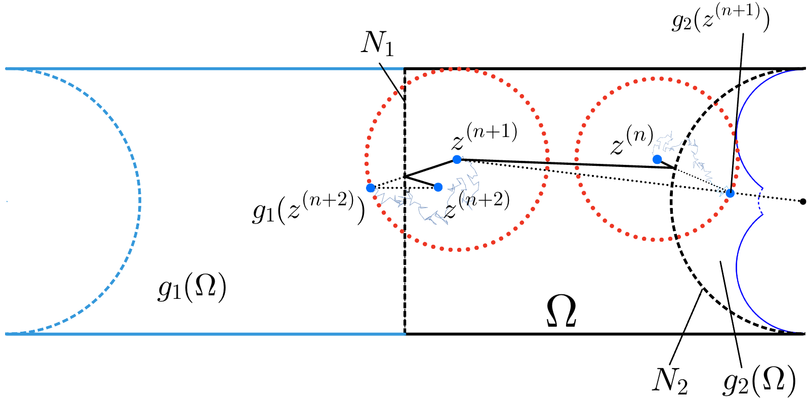
In the Dirichlet–Neumann problem the Brownian trajectory is absorbed in the Dirichlet boundary and reflected on the zero-valued Neumann boundary. The challenge in applying the WoS algorithm in solving the 2d Dirichlet–Neumann problem is to accurately reflect the Brownian motion at Neumann boundaries. One idea is that, when the particle is near the Neumann boundary, stop walking on spheres and use the primitive idea of simulating fine time mesh to compute the reflection angle about the normal lines. But this is not only very costly in computation, but also it brings in an error dependent on step size in the simulation. Therefore, the idea of fine time mesh to simulate reflection is not very desirable. Fortunately, for Neumann boundaries that are straight segments, we can think of them as mirrors and walk on spheres through the mirrors as if there is no barrier between our real world and the reflected imaginary world. As soon as the Brownian particle stepped into the reflected domain, we bring it back by reflecting it about the straight Neumann boundary, just as if it had bounced off the mirror (maybe more than once). In this way, we have walked on a sphere not bounded by the Neumann boundary. Although we don’t know the exact reflection process the particle went through, we have simulated the destination point at a macroscopic level. And then we set this destination point as the center for the next sphere walk.

In addition of straight lines, we also consider curved Neumann boudaries. The reflection with respect to curved boundaries are handled by using anti-conformal mappings.

In the following $N\subseteq\Gamma_{N}\subseteq\partial\Omega$ is a curved Neumann boundary.

1. (1)

   Find the conformal mapping $f$ that transform $N$ into a straight line segment $I$.

2. (2)

   Find the reflection function $R$ about the line segment $I$.

3. (3)

   Then the composition function $g=f^{-1}\circ R\circ f$ is the desired anti-conformal mapping which mirrors $\Omega$ into the reflected domain $g(\Omega)$. Since only the set $N$ remains fixed in the reflection, it would be expected $\Omega\cap g(\Omega)=N$.

In addition, $g=g^{-1}$ since

Therefore, $g(g(\Omega))=\Omega$.

The remaining question is how to find the conformal mapping $f$ from curved boundary to line segment. This is a difficult question and there is no general answer yet. However, this issue is mitigated for circular-arc boundaries for which we have the well-known Möbius transformations that can map circles into lines.

If we use the composition mentioned above, for circular-arc boundaries with radius $R$ centered at $(x_{1},y_{1})$, the mapping

is the anti-conformal reflection. This mapping is an inversion in $S((x_{1},y_{1}),R)$ and hence preserves the class of generalized circles[5, Theorem 3.2.1]. Thus the reflections at circular-arc Neumann boundary are manageable.

We first test our method on the simplest canonical domain, which is the rectangle $\{z\in\mathbb{C}:0<\operatorname{Re}(z)<h,0<\operatorname{Im}(z)<1\}$. By Definition 2.1, the modulus of the normalized rectangle is its height $h$.

The L-shaped region

is commonly used in various computational analyses. It has been explored by Gaier [9], who provided computed moduli values for such domains. We compare our results with his.

Given four distinct points $z_{1},z_{2},z_{3},z_{4}$ in the complex plane $\mathbb{C}$, the cross-ratio is defined by the expression:

An important property of the cross-ratio is its invariance under Möbius transformations. That is, if $T$ is a Möbius transformation, then the cross-ratio of the transformed points $T(z_{1}),T(z_{2}),T(z_{3}),T(z_{4})$ remains unchanged:

Type A. Consider a quadrilateral with sides formed by circular arcs from intersecting orthogonal circles, where angles are $\pi/2$. Let $0<a<b<c<2\pi$ and select points $\{1,e^{ia},e^{ib},e^{ic}\}$ on the unit circle. The absolute value of the cross-ratio of these four points is

Define $Q_{A}$ as the domain obtained from the unit disk by removing regions bounded by two orthogonal arcs with endpoints $\{1,e^{ia}\}$ and $\{e^{ib},e^{ic}\}$ respectively, forming the quadrilateral $(Q_{A};e^{ia},e^{ib},e^{ic},1)$. By applying an appropriate Möbius transformation, we are able to conformally map the quadrilateral $Q_{A}$ onto the upper semicircle of the annulus $\{z\in\mathbb{C}:1<|z|<t\}$ in the complex plane. The conformal modulus of the annulus $\{z\in\mathbb{C}:1<|z|<t\}$ is $(2\pi/\log t)$ [9]. Therefore the modulus of the quadrilateral is precisely half that of the full annulus,

with:

The contours of the two potential functions are shown in Figure 8. The computed values of the moduli are in Table 3.

Type B. Consider the sides of the quadrilateral as circular arcs within the unit disk, where each internal angle is $\pi$. Consequently, the unit disk, along with the boundary points $\{e^{ia},e^{ib},e^{ic},1\}$, defines a quadrilateral, which we denote as $Q_{B}$. Again, by employing a proper Möbius transformation to map the unit disk onto the upper half-plane, we can conveniently express the modulus using the capacity of the Teichmüller ring domain [4, Section 7]. This is formulated as:

where $u$ is defined as in equation (14), and

Here, $\mu_{1/2}(r)$ is defined in [15, Subsection 4.3]. The summarized results are presented in Table 4, The contours of an example are shown in Figure 10.

In higher dimensions, our method has particular appeal due to its relative simplicity when compared to alternative solutions. The reflected WoS algorithm extends naturally to 3D Dirichlet–Neumann domains, modeling insulated heat flow in thermodynamics. See Figures 12 and 13.

References

- [1] M. Abramowitz and I. A. Stegun, Handbook of mathematical functions with formulas, graphs, and mathematical tables, vol. No. 55 of National Bureau of Standards Applied Mathematics Series, U. S. Government Printing Office, Washington, DC, 1964. For sale by the Superintendent of Documents.
- [2] L. Ahlfors, Conformal Invariants: Topics in Geometric Function Theory, McGraw-Hill Book Co., 1973.
- [3] , Lectures on quasiconformal mappings, vol. 38 of University Lecture Series, American Mathematical Society, Providence, RI, second ed., 2006. With supplemental chapters by C. J. Earle, I. Kra, M. Shishikura and J. H. Hubbard.
- [4] G. Anderson, M. Vamanamurthy, and M. Vuorinen, Conformal invariants, inequalities, and quasiconformal maps, (1997).
- [5] A. F. Beardon, The Geometry of Discrete Groups, Graduate Texts in Mathematics, Springer New York, NY, 1 ed., 1983.
- [6] P. Bowers and M. Hurdal, Planar conformal mappings of piecewise flat surfaces, Visualization Math. III, (2003), pp. 3–34.
- [7] W. Calixto, B. Alvarenga, J. da Mota, L. da Cunha Brito, M. Wu, A. Alves, L. Neto, and C. Lemos Antunes, Electromagnetic problems solving by conformal mapping: A mathematical operator for optimization, Mathematical Problems in Engineering, 2010 (2011), p. e742039.
- [8] T. Driscoll and L. Trefethen, Schwarz-Christoffel mapping, vol. 8 of Cambridge Monographs on Applied and Computational Mathematics, Cambridge University Press, Cambridge, 2002.
- [9] D. Gaier, Conformal Modules and their Computation, World Scientific, River Edge, NJ, 1995, pp. 159–171.
- [10] J. Garnett and D. Marshall, Harmonic Measure, Cambridge University Press, 2005.
- [11] F. González-Matesanz and J. Malpica, Quasi-conformal mapping with genetic algorithms applied to coordinate transformations, Computers & Geosciences, 32 (2006), pp. 1432–1441.
- [12] X. Gu and S.-T. Yau, Computational conformal geometry, vol. 3 of Advanced Lectures in Mathematics (ALM), International Press, Somerville, MA; Higher Education Press, Beijing, 2008. With 1 CD-ROM (Windows, Macintosh and Linux).
- [13] H. Hakula, T. Quach, and A. Rasila, Conjugate function method for numerical conformal mappings, Journal of Computational and Applied Mathematics, 237 (2013), pp. 340–353.
- [14] H. Hakula, T. Quach, and A. Rasila, The conjugate function method and conformal mappings in multiply connected domains, SIAM J. Sci. Comput., 41 (2019), pp. A1753–A1776.
- [15] H. Hakula, A. Rasila, and M. Vuorinen, On moduli of rings and quadrilaterals: algorithms and experiments, SIAM J. Sci. Comput., 33 (2011), pp. 279–302.
- [16] , Computation of exterior moduli of quadrilaterals, Electron. Trans. Numer. Anal., 40 (2013), pp. 436–451.
- [17] , Conformal modulus and planar domains with strong singularities and cusps, Electron. Trans. Numer. Anal., 48 (2018), pp. 462–478.
- [18] P. Henrici, Applied and Computational Complex analysis. Vol. 3: Discrete Fourier Analysis—Cauchy Integrals—Construction of Conformal Maps—Univalent Functions, John Wiley & Sons, Inc., USA, 1986.
- [19] S. Kakutani, Two-dimensional brownian motion and harmonic functions, Proceedings of the Imperial Academy, 20 (1944), pp. 706–714.
- [20] L. Kharevych, B. Springborn, and P. Schröder, Discrete conformal mappings via circle patterns, ACM Trans. Graphics (TOG), 25 (2006), pp. 412–423.
- [21] S. Krantz, Geometric function theory: Explorations in Complex Analysis, Cornerstones, Birkhäuser Boston, Inc., Boston, MA, 2006.
- [22] P. Kythe, Handbook of conformal mappings and applications, CRC Press, Boca Raton, FL, 2019.
- [23] G. Lawler, Conformally invariant processes in the plane, vol. 114 of Mathematical Surveys and Monographs, 2005.
- [24] O. Lehto and K. Virtanen, Quasiconformal Mappings in the Plane, Springer, Berlin, 1973.
- [25] S. Maire and E. Tanré, Monte Carlo approximations of the Neumann problem, Monte Carlo Methods and Applications, 19 (2013), pp. 201–236.
- [26] M. Mascagni and C.-O. Hwang, -shell error analysis for ”walk on spheres” algorithms, Mathematics and Computers in Simulation, 63 (2003), pp. 93–104.
- [27] M. Muller, Some continuous Monte Carlo methods for the Dirichlet problem, Ann. Math. Statist., 27 (1956), pp. 569–589.
- [28] M. Nasser, Numerical conformal mapping via a boundary integral equation with the generalized Neumann kernel, SIAM J. Sci. Comput., 31 (2009), pp. 1695–1715.
- [29] M. Nasser, O. Rainio, A. Rasila, M. Vuorinen, T. Wallace, H. Yu, and X. Zhang, Polycircular domains, numerical conformal mappings, and moduli of quadrilaterals, Adv. Comput. Math., 48 (2022), pp. Paper No. 58, 34.
- [30] M. Nasser and M. Vuorinen, Isoperimetric properties of condenser capacity, Journal of Mathematical Analysis and Applications, 499 (2021), p. 125050.
- [31] N. Papamichael and N. Stylianopoulos, Numerical Conformal Mapping: Domain Decomposition and the Mapping of Quadrilaterals, World Scientific Publishing Company, 2010.
- [32] R. Schinzinger and P. Laura, Conformal Mapping: Methods and Applications, Dover Publications, Inc., Mineola, NY, revised edition ed., 2003. Revised edition of the 1991 original.
- [33] K. Stephenson, Introduction to Circle Packing: The Theory of Discrete Analytic Functions, Cambridge University Press, Cambridge, 2005.
- [34] M. Vermeer and A. Rasila, Map of the World; An Introduction to Mathematical Geodesy, CRC Press, Boca Raton, FL, 2020.
- [35] Y. Wang, X. Yin, J. Zhang, X. Gu, T. Chan, P. M. Thompson, and S.-T. Yau, Brain mapping with the Ricci flow conformal parameterization and multivariate statistics on deformation tensors, in 2nd MICCAI Workshop on Mathematical Foundations of Computational Anatomy, 2008, pp. 36–47.
- [36] R. Wegmann, Chapter 9 - methods for numerical conformal mapping, in Geometric Function Theory, R. Kühnau, ed., vol. 2 of Handbook of Complex Analysis, North-Holland, 2005, pp. 351–477.
- [37] X. Yang, A. Rasila, and T. Sottinen, Walk on spheres algorithm for Helmholtz and Yukawa equations via Duffin correspondence, Methodol. Comput. Appl. Probab., 19 (2017), pp. 589–602.
- [38] , Efficient simulation of the Schrödinger equation with a piecewise constant positive potential, Math. Comput. Simulation, 166 (2019), pp. 315–323.