Mohammed S. Al-Mahfoudh and Ryan Stutsman,
Efficient Linearizability Checking for Actor-based Systems
Abstract
[Summary]Recent demand for distributed software had led to a surge in popularity in actor-based frameworks. However, even with the stylized message passing model of actors, writing correct distributed software is still difficult. We present our work on linearizability checking in DS2, an integrated framework for specifying, synthesizing, and testing distributed actor systems. The key insight of our approach is that often subcomponents of distributed actor systems represent common algorithms or data structures (e.g. a distributed hash table or tree) that can be validated against a simple sequential model of the system. This makes it easy for developers to validate their concurrent actor systems without complex specifications. DS2 automatically explores the concurrent schedules that system could arrive at, and it compares observed output of the system to ensure it is equivalent to what the sequential implementation could have produced. We describe DS2’s linearizability checking and test it on several concurrent replication algorithms from the literature. We explore in detail how different algorithms for enumerating the model schedule space fare in finding bugs in actor systems, and we present our own refinements on algorithms for exploring actor system schedules that we show are effective in finding bugs.
keywords:
Model Checking, Actor Model, Distributed Systems, Fault ToleranceRecent years have seen a surge in actor-based programming. This is, in part, because many applications today are naturally concurrent and demand some means for distribution and scale-out. Hence, actor-based frameworks 1, 2, 3, 4 have seen large-scale production deployment 5, 6 running real, low-latency services for thousands to millions of concurrent users. However, despite a stylized message-passing-based concurrency scheme that avoids the complexity of shared memory, actor systems still contain bugs 7. As a result, prior works have sought to bring model checking techniques 8, 9 and code coverage-driven techniques 7 to bear on these systems with some success.
However, beyond exploring schedules efficiently, a separate challenge is the more basic problem of specifying invariants and safety properties for these types of complex systems 10, 11. One approach that has gained traction in recent years is manual, black-box testing of systems under complex, concurrent scenarios and comparing against a simple, sequential reference implementation that meets the same interface as the complex, concurrent system 12. For example, recording and checking the linearizability 13 of a history of responses produced by the larger system against responses produced by the reference implementation provides a sound and complete means for testing a single, particular execution schedule of the system 14, 15. The problem with this approach is that if interesting schedules are missed by the user testing the system or if certain schedules are hard to produce, then this approach says little about the overall correctness of the system.
Our goal is to combine the success of these two techniques (schedule exploration and linearizability checking) in an automated package for actor systems. These systems often contain subcomponents that provide concurrent implementations of abstract data types (ADTs) with well-defined inputs and outputs (invocations and responses). Hence, these subcomponents are amenable both to exhaustive schedule generation and to automated testing against reference implementations of the corresponding ADTs. This new approach provides a richer set of checks than simple schedule exploration against user-specified assertions while maintaining simplicity of user provided specification. Of course, to be practical, such an approach must control explosion both in schedule exploration and in history checking costs.
As a first step toward this goal, this paper attempts to understand how best to control that explosion by assessing the performance of many classic and state-of-the-art schedule exploration algorithms when considered together with state-of-the-art linearizability checking algorithms. To that end, we compare several algorithms on multiple actor systems. For example, we test with a simple distributed register and compare checking costs when that same ADT is lifted for fault tolerance using standard consensus-based state machine replication protocols 16, 17, 18. This shows that beyond testing individual systems, this approach also works as an easy approach to testing these notoriously subtle black-box replication techniques. Ultimately, we show that by 1) subdividing systems by the principle of compositionality of linearizability 19, 14, 13 and 2) exploiting independence between actors for effective dynamic partial order reduction (DPOR) 8, 20, we can limit the number of schedules to make finding bugs in concurrent actors systems practical by comparing against a simple, sequential reference implementation of the system’s ADT.
Beyond this first step, our analysis informs a larger effort on our framework, an actor-based framework for specifying and checking distributed protocols. It provides a concise language for specifying systems, and using our framework, users can manually drive testing on their systems (the framework includes some specialized schedulers specifically for this kind of test-driven checks), can rely on its automated schedule exploration and linearizabilty checking, or can extend its automated schedulers. Our end goal is an easy system for specifying and testing distributed actor systems that can drive synthesis to practical implementations.
In sum, this paper makes the following contributions:
-
•
Our framework 21 that not only made our schedulers fully stateful111Saving the entire state of the distributed system in order to back track to it during exploration, instead of the previous implementations of algorithms that re-run the system controllably from start to end., extensible222Both hierarchies of schedulers/algorithms and distributed system model are extensible independently and they will still be compatible with each other., re-usable333Class hierarchies are modularily structured that one can override few methods while keeping the rest intact and still be re-usable., composable444Schedulers can be composed, nested, and can save the state and do hand-off between themselves without having to restart explorations., and modular555Schedulers are structured in a way that all their behavior is overridable in parts or in whole without having to re-write all parts of the scheduler e.g. the main loop. but also reduced our novel algorithms/schedulers implementations to mere predicates on receives (i.e. didEnable(receive1,receive2) and areDependent(receive1,receive2)), one for each of our algorithms. These features make schedulers and the networked distributed system model (the context) simple for developers to extend. practically. The novelty in this work does not stop at an almost no overhead algorithm to dynamically detect causality between events (zero memory overhead, and almost no compute overhead per the experiments) and at the same time deduplicating retries. It goes beyond that with a unique declarative environment for exploring actor systems in Scala. This promotes formalism in software practice.
-
•
An automated approach to correctness testing of subcomponents of actor systems no developer-provided specification aside from a simple, non-concurrent (i.e. sequential) specification reference implementation of the component and a simple test harness.
- •
- •
-
•
A detailed comparison of these algorithms used for the first time in the context of linearizability checking instead of simple invariant checking, run side-by-side on the same benchmarks showing how they perform and scale when checking actor systems. This helps show effectiveness of focusing schedule generation towards revealing linearizability violations.
1 Background
1.1 Actor Systems
Actors are a model for specifying concurrent systems where each actor or agent encapsulates some state. They do not share state and have no internal concurrency666Internal concurrency is any concurrency inside a single actor e.g. multithreading. An actor is strictly a sequential communicating process. Mixing multithreading breaks the actor model’s encapsulation.. Instead, actors send and receive messages between one another. Internally, each actor receives an incoming message and performs an action associated with that message. Each action can affect the actor’s local state and can send messages to other/same actor(s). Each actor executes actions sequentially on a single thread, but an actor system can run concurrent and parallel actions since the set of receiving actors collectively perform actions concurrently.
By eliminating complex constructs like threading and shared memory, actors make it easier for developers to reason about concurrency. For example, data races777We distinguish between a data race (which is a race condition over the data in the local state of an actor) and a race condition (which is any non-deterministic behavior due to the order in which events are processed) are impossible in actor systems. However, race conditions can manifest in the order of the messages received by the actor in case they interfere. This programming model naturally supports distribution, since it relies on message passing rather than shared memory. As a result, there are many popular actors frameworks 1, 3, 35, 36, 37 that closely adhere to the actor model.
1.2 Model Checking
Model checking has been applied in many domains to assess the correctness of programs 38, 39, 40, 41, 42. This includes actor systems 8, real-time actor languages 43, and the Rebeca Modeling Language 44. Model checkers explore states a system can reach by systematically dictating different interleavings of operations (each of which is called a schedule). In actor systems, concurrency is constrained by the set of sent-but-unreceived messages in the system, which determines the set of enabled actions at each point in the execution. Hence, it consists of exploring the set of all possible interleavings of message receives.
This brings the issue that we are assuming a hand-shake driven model. This is true, but our model (and its operational semantics rules) is not limited to that, as it offers timed actions (real time, since it is executable, or relative ordering) for blocking and non-blocking actions. However, since that would need users’ modulation of input application times, schedulers do not implement this yet.
In model checking, exploration is typically coupled with a set of invariants or assertions provided by the developer of the system under check. By checking that the invariants hold in all states reachable via any schedule, developers can reason about safety and/or correctness properties of their program.
Many different strategies have been explored for guiding schedule enumeration or reducing its inherent exponential cost. Ultimately, for non-trivial programs model checkers cannot enumerate all schedules and must bound exploration; hence, this may lead to algorithms that are sound but with incomplete results, i.e. not complete state space coverage. Randomized scheduling has shown promise, since it explores diverse sets of schedules. Another approach is dynamic partial order reduction (DPOR) 20, which prunes schedule enumeration by only exploring enabled actions that could interfere888We say messages “interfere” when they are received by the same actor and their effects do not commute. Similarly in threads, two operations interfere when there is a write operation whose effect(s) does not (do not) commute with another write/read operation. with one another. This has been extended to the context of actor-based systems where the extra independence between actions (due to the lack of shared memory) allows additional pruning 8. We describe several of these strategies in more detail in Section 2.
Importantly, before a developer can use a model checker to check their code for correctness, they must first specify properties that the scheduler should check as it explores systems’ states. This is a challenge for most developers, especially in concurrent systems.
1.3 Linearizability
Linearizability is a consistency model for concurrent objects (e.g. registers, stacks, queues, hash tables) 13. Linearizability has several key properties that makes it common and popular in distributed programming. It is strict about ordering, which eases reasoning, but it allows enough concurrency for good performance.
From the perspective of an object user (or a system representing it), each operation they invoke appears to happen atomically (instantaneously) between the time of its invocation until the time of its response, a linearization point in time. Because operations take effect atomically, i.e. totally orders them, the concurrent object has a strong relationship to a sequential counterpart of the same ADT. For some history of operations (a sequence of invocations and responses) on that object, there must be a total order of those operations that when applied to a sequential implementation of the same ADT produces the same responses. This is powerful because any sequential implementation can be used to cross-check the responses of a concurrent implementation against its sequential counterpart.
(Rd); (0); (Wr, 1); (); (Rd); (1)
(Rd); (Wr, 1); (); (Rd); (1); (0)
Figure 1 visualizes a sequential history of operations on a register that supports a read and write operation. Figure 2 shows a concurrent history using the same abstract type (a register). The operations overlap and run concurrently, but the register produces the same response to each of the invocations as the history in Figure 1. Hence, the concurrent register executed the operations in a consistent manner to the sequential counterpart. The user can reason about concurrent operations on the register in similar way to that of a sequential implementation protected by a mutex. For example, in Figure 2 res1 could return 1, in which case the execution would be equivalent to a different sequential history; this is okay. However, res3 could never return 0, since no sequential history where inv3 happens after the completion of res2 could explain that result; otherwise, this would indicate a bug in the concurrent implementation. Importantly, all of this can be understood by observation only, and basic understanding of the equivalent sequential reference implementation (for invocations vs responses).
Linearizability Checking and WGL Algorithm 45. This correspondence between sequential and concurrent histories is what enables automated detection of bugs in concurrent objects. To do this, one can capture a history of operations from a concurrent structure. Feeding these operations one-at-a-time into a sequential structure, say, in invocation order may produce the same return values for each response, in which case the captured history is consistent with linearizability. However, this might not work because the concurrent execution may lead to different responses orderings. Even repeating the same procedure in response order can be fruitless. Only an exhaustive search over the space of potential equivalent histories may yield a correspondence. WGL algorithm 45 generates these permutations which are all of the same history that 1) never reorders a response before its invocation, and 2) never reorders two invocations. For each sequential history it finds (a history where each invocation is adjacent to its response) it feeds the history to a sequential implementation of the ADT being checked to see if all the responses match. If some sequential history that explains the concurrent one is discovered, then the implementation being checked behaved in agreement with linearizability in the execution described by that one history. Otherwise, the history is deemed non-linearizable.
2 Overview
The focus of this paper is to explore model checking in the context of linearizability checking. That is, model checking can be used to systematically produce histories. When put together, these techniques would let developers check full, concurrent actor systems for correctness without manual specification of invariants. The key problem is that both algorithms are exponential; however, this says little about the potential usefulness of combining the techniques. Past works have proposed many ways to reduce schedules to explore. No prior work explores how these different schedulers impact the set of histories to check when exploring a structure, nor does any prior work explore the interplay between model checking costs and history checking costs. Hence, we begin our efforts to improve linearizability checking costs for practical actor-based systems with a quantitative exploration of existing techniques. Later, we describe our own new schedulers designed to improve over them.
2.1 Toolchain Flow

Figure 3 shows our setup for checking actor systems. The user specifies an actor-based system that represents some ADT (e.g. a map) as an instance of our executable model.
In our approach, each scheduler starts with a set of messages destined to a set of actors. For each of these messages we say a destination’s receive is enabled. At each step, a scheduler’s job is to choose an enabled receive from the enabled set, to execute the action associated with it on the destination actor, and mark the receive explored so that it will not be revisited from that specific state. Later, the scheduler may need to backtrack to that state so it explores other interleavings of remaining receives. Before executing a receive and after marking it as explored, a scheduler snapshots the entire system state and the different sets of receives.
To start checking an implementation, a user provides the actor system that implements the ADT, and a set of invocations on it. Our Schedulers use these harnesses to inject these invocations as messages before the scheduler starts, then it starts exploring till no more enabled receives remain. Response messages accumulate in a client’s queue to be appended to the schedule, by the scheduler.The sequence of invocations and responses it discovers form histories999Note that even schedules that lead to these histories are accessible in a construct in the schedulers until the exploration statistics are printed..
2.2 Schedulers
Here, we describe the set of schedulers we compared starting with the simplest ones. The criteria for choosing these 7 algorithms is multifaceted: 1) they are popular, 2) all extend each other towards specialization in a linear inheritance (i.e. to implement LiViola – LV – we had to implement all that it refines/inherits) which reduces the amount of duplicated code and increases modularity; and 3) they form a basis for many other algorithms to extend and specialize them as needed.
2.2.1 Systematic Random (SR)
From the initial enabled set, the systematic random scheduler chooses a random receive and executes it. This may enable new receives to add to the previously enabled ones to pick from, and the process repeats until no enabled receives remain. From there, the scheduler backtracks to the initial state and initial enabled set and repeats until a timeout.
2.2.2 Exhaustive DFS (Depth First Search)
One straightforward approach to exploring systems is to explore schedules depth first. This algorithm non-deterministically picks an enabled receive that has not been marked explored and performs the associated action. When the enabled set is empty on some path, it outputs a schedule which later is transformed into a history. Then, it backtracks to the earliest point in time where other, unexplored, receives remain and it repeats this procedure. To bound execution time, all schedulers have to be stopped at some point, e.g. at some count of schedules generated. Hence, in practice, this policy will tend to mostly make some initial choices of receives, and it will aggressively explore reorderings of the “deepest” enabled receives before timing out. As a result, in our experience, this approach tends to explore similar schedules (before timing out), so it produces many but similar histories.
All of the remaining schedulers are based on Exhaustive DFS. They cut the search space by overriding methods that refine the scheduler behavior to prune receives causing redundant schedules/histories.
2.2.3 Delay-bounded (DB)
The delay-bounded scheduler 46 extends the Exhaustive DFS scheduler, and it mainly explores schedules similarly but randomly delaying some receives. The scheduler starts with a fixed delay budget . As it explores, for each receive , it picks a random natural number d, . If then the scheduler skips over agents that have enabled receives in the enabled set in a round robin order, and it explores the next agent’s enabled receive. The sum of chosen values of along in a schedule is bounded to .
2.2.4 Dynamic Partial Order Reduction(DPOR/DP)

Dynamic partial order reducing (DPOR 20) scheduler prunes schedules that reorder independent receives that affect different actors. If two receives target the same actor, then they are considered dependent since the order they are applied in can influence the behavior of that agent (and transitively those it communicates with). In Figure 4, for example, when exploring a state of the system, there are two enabled receives; destined to agent and destined to agent . The scheduler picks one of them non-deterministically (here ), and it executes the transition, producing destined to . In the new state, it then chooses to execute . Notice that and are independent so only one interleaving needs to be explored. However, when is chosen and executed, the scheduler notices that the previously chosen is dependent, so it determines that it must explore the receives in the opposite order as well. Hence, the scheduler first checks if is enabled in the state from which was executed. If so, it adds it to the first state’s backtracking set, which tracks the remaining receives that need be explored after completing the current path. It only needs to do costly branching if the receives are dependent.
One complication arises in DPOR (shown in Figure 4) is that it is possible that is not in the enabled set of the top state (labeled start). That is, two receives can be dependent, but they might not always be in one enabled set. This situation is due to a later executed receive enabling . In that case, DPOR takes all receives that executed between the dependent state (i.e. a previous state from which a receive destined to the same agent as the current receive was executed) and the current one, and filters them based on whether they were enabled in the dependent state, returning only those that were enabled in the dependent state. Then, the entire set of filtered receives is added to the dependent state’s backtracking set to explore later. This is where TransDPOR and IRed improve over DPOR, by being more careful about which one from the filtered set of receives is added to the dependent state’s backtracking set.
2.2.5 TransDPOR (TD)
The key idea in TransDPOR 8 that differentiates it from DPOR is that when a receive becomes enabled that is dependent with a receive earlier in the schedule, it is added to the backtracking set of that earlier state (the dependent state) in the schedule only if that state’s backtracking set is empty. TransDPOR always over approximates the root enabler receive (the receive that enabled the current one whether directly or transitively) by always adding the first receive in the schedule after the one executed from the dependent state to the dependent state’s backtracking set.
2.2.6 IRed (IR)
IRed is based on TransDPOR, and improves over it in one specific aspect. It tracks causality (i.e. the root enabler receive) with perfect precision by scanning for the causal chain backwards starting from the current receive until the first one that enabled it in the schedule. Then it adds that root enabler receive, if found, to the dependent state’s backtracking set. Otherwise, if a root enabler was not found, it does not update the backtracking set. More concretely, during the scan, it checks for the predicate (and keeps track of the earliest receive executed in the schedule that satisfies it) whether the current receive’s sender is the same as the previous receive’s receiver. The earliest receive that satisfies it becomes the current root enabler receive. The scanner continues in this manner until it reaches the dependent state, or the predicate is no more satisfied and the last root enabler receive detected was enabled (co-enabled) in the dependent state. In which case, the last root enabler receive is the the one to explore when the algorithm backtracks to that specific state. The sequence of receives starting at the root enabler up to and including the current receive is called causal chain, and the root enabler is the first receive in this sequence. This causal chain pattern is characteristic of actors and purely sequential communicating processes. This reverse traverse for the root enabler also filters away many unrelated receives effectively, and it improves backtracking in the presence of retries. This is where our algorithm thrives in complexity that is common in distributed systems.
2.2.7 LiViola (LV)
Our second algorithm is based on IRed and is focused on revealing linearizability violations by redefining the dependence relation of concurrent key-value stores. Linearizability is compositional 14, 13, 47. However, the only time this was exploited for verifying linearizability is in P-Compositionality work 14 at the history level. In addition, we realized that a linearizability violation is a race condition on an actor/agent having two interfering receives (due to network re-ordering) or transitively between the actors/agents composing the distributed ADT (and, hence, a data race on the collective state of actors composing the ADT) that is exposed clients. We used this fact to restrict the number of interesting schedules that may produce linearizability bugs by applying it at the schedule generation stage. This was done by first augmenting the harness with additional internal messaging info, and then overriding the dependence relation to restrict dependent states to those that satisfy all of the following: (1) the receive executed from that state has to be targeting the same agent/receiver (same as before); and (2) the receives have to target a certain key in the distributed key-value store (compositionality of linearizability). So, the hypothesis about our algorithm (LiViola) is that it is expected to perform the worst in a single key-value store (e.g. a map that has one key, a register, or a single element set) and perform the best as more keys are added to the distributed ADT. Hence, our two algorithms above should thrive on complexity more than the other algorithms. In addition, it is noted in WGL paper 45 that WGL suffers the most when there are more keys; however, our algorithms should reduce the number of schedules the most when there are more keys. In other words, the more WGL has to deal with more keys interleaving, the fewer schedules our algorithms produce in comparison to others and the more complimentary they are to WGL checking.
While IRed algorithm’s improvement is generic to all problems, LiViola is specialized to linearizability. As a result, IRed enables a whole class of algorithms that extend it and can be specialized in-lieu LiViola to more precisely address different problems. That can be done by overriding one/both of the and methods.
3 Algorithms in Detail
In this section, we begin with a visual walk through of the TransDPOR and IRed algorithms in order to visually spot the differences. After that, in next section §3.1, we present the differences between them in the form of pseudocode walk through to remove any confusion, and to make it easier to code the algorithms.


Here, we start by explaining the symbols shown in Figures 5 and 6. Ovals represent states, and arrows represent the transitions (receives) that are executed from one state and lead to the transition to the next state. Different sets are represented with two/three letters: The Enabled Set is referred to as EN , The Explored Set (the done set) is symbolized as EX , and the pending set is referred to as PND (it is ), and finally the Backtracking Set is referred to as BT . The pending set represents the enabled receives that have not been explored from the specific state; hence, they are enabled but not in explored/done set. It is made explicit to simplify understanding and to relate to the pseudocode in the next subsection when we explain algorithms in more detail.
First, we explain TransDPOR visually. Initially, there are two requests (receives) from two different clients (shown in the enabled set to the left and right of state 0 in Figure 5), shown in the enabled set and the pending set is equal to the enabled set. Once the algorithm randomly picks receive m1a (i.e. message m1 heading to agent a), it adds it to the explored set ( EX ) and that leads to removing it from the pending set. It executes the receive, transitioning from state 0 to state 1, that has the corresponding set shown to its left and enabling receive m3a, i.e. by executing the action to process m1a and that action has a send statement that sends out m3a. The algorithm proceeds by doing the same, now randomly choosing to execute receive m1b, and ending at state 2. It continues the same way but now the algorithm detects that the current receive (m3a) is dependent with a previous receive (namely m1a); since they are heading to the same agent (agent a).
Now the algorithm does two checks. In the first check, it checks if the current receive m3a was co-enabled (resides in the same enabled set of the state from which the dependent receive was executed, i.e. state 0). It does not; hence, it was not co-enabled with the receive m1a, so the algorithm cannot update the backtracking set of state 0 to contain the current receive. In the second check, the algorithm goes to try another option to update the backtracking set (to explore another possible interleaving). TransDPOR picks the first receive after the dependent receive (symbolized as pre(S,i) in the next section pseudocode) and assumes it is the receive that enabled the current receive m3a whose sender is agent/actor a. That receive (m2b) is then added to the backtracking set of state 0 to be explored upon backtracking to that state. TransDPOR, at this stage, locks the backtracking set of state 0 by setting a freeze flag, meaning that no more receives are allowed to be added to that specific backtracking set (that is part of state 0). Hence, it keeps the backtracking set size to a maximum of one receive at any time. This is how it narrows down the exploration tree in comparison to the original DPOR that adds more than one receive at a time to a certain backtracking set. TransDPOR then executes the transition/receive (m3a) ending in state 3. At this stage, there are no more pending/enabled receives that the algorithm can execute, so it backtracks until it reaches a state where the backtracking set is not empty. That is, state 0 at this point.
Once it is at state 0, it detects that the backtracking set is not empty, so it unfreezes (sets the freeze flag to false) the state, picks the m2b receive and executes it transitioning to state 4. It continues in a similar manner until it reaches state 6, and after that, it backtracks and exits since no more backtracking sets are updated. In the next paragraphs, we explain IRed operation on the same input.
After explaining TransDPOR, we explain IRed algorithm in a similar manner. IRed execution of the system proceeds exactly as TransDPOR up until state 2. At state 2, it does the first step exactly like TransDPOR does, i.e. it checks if m3a is co-enabled with m1a in state 0, but it finds it is not. Then, the second option, it tries to find the root enabler (i.e. the receive that originally, directly or transitively, enabled receive m3a). The way IRed does it is different from TransDPOR. TransDPOR, as we saw earlier, assumes that the first receive after the dependent receive (dependent receive being m1a and m2b is the one after it in this example) is the one that enabled m3a. We know this is not true, and it is an imprecision of TransDPOR. IRed, however, is precise at picking the root enabler. It scans backwards, checking if the sender of receive m3a (we write it as ) is the same receiver of m2b (we write it as ). The key idea here is that if m3a was sent by agent/actor b and m2b was the last receive received by agent b (same agent), then receiving m2b could have triggered agent b to send m3b. Hence, the root enabler receive becomes m2b. At this stage, it is not true that m2b is the root enabler since m3a was sent by agent a not agent b. However, we reached the dependent state so the algorithm can not check the same predicate for the current receive versus the dependent receive (i.e. ) since they are not co-enabled in the first place and the algorithm has no benefit at running dependent receive itself, m1a, again from the same state so it stops before doing so. If they were co-enabled, however, m3a would have been added to state 0’s backtracking set before the algorithm takes this second scenario/step of the algorithm.
Elaborating more, assume there was another earlier executed receive (call it m2a) after the dependent receive, and now the earlier receive and current one satisfy the predicate above. The algorithm then makes the earlier receive (m2a) the current one, and it proceeds until it reaches the dependent receive. The latest current receive tracked by IRed, is then checked if it was co-enabled with the dependent receive m1a. If it is, it is added to state 0’s backtracking set; otherwise, it is not added. To elaborate on the same example, assume there are hundred retries of the same receive m2a, i.e. the message m2a was sent a hundred times. There are two scenarios on how the algorithm deals with this situation. The first scenario is that the sender of these m2a retries is agent a itself, in which case the algorithm picks the earliest one, as we saw in the example, as the root enabler. The second scenario is that retries of m2a were sent by another agent, say b, in which case the algorithm will pick the latest one, as in closest to current receive, as the new current receive (candidate root enabler) and filters away all earlier ones. The reason why the other 99 retries are skipped is that they do not satisfy the IRed predicate. For example, the 99th m2a does not have the same receiver (agent a) as the 100th m2a’s sender (agent b in the second scenario), and such is the case with the rest of retries. It skips 99 retries, and it resumes from that point on until reaching the dependent receive and proceeds similar to previously explained. Hence, it de-duplicates all these retries that represent a common communication pattern in distributed systems. Other algorithms, e.g. TransDPOR, would suffer the classic state space explosion problem in this case.
In the next section (§3.1) we elaborate with more detail these differences, define all the terms used, and redefine a few relations to address both differences in TransDPOR, IRed, and LiViola.
3.1 The Pseudocode Walk Through
In this section we present IRed pseudocode in detail and will contrast it to TransDPOR and LiViola. The algorithm shows the difference between TransDPOR, IRed, and LiViola. The differences between TransDPOR and IRed are underlined, while between LiViola and all others (including IRed) are double underlined. However, before we can understand the algorithm, we need to explain some primitives and notations. We keep most notations the same as in TransDPOR paper 8 to simplify understanding.
3.1.1 Notations, Terms, and Definitions
As explained in our operational semantics paper 32, the global state of an actor system is a distributed system state in DS2 terms, and here it is symbolized as , where is the set of all possible states in a system. Each state is comprised of a map where is the set of all possible agents/actors identifiers in the system, and are possible local states. In that state, is the set of all pending messages, while is the set of all possible messages in the system.We, also, use to indicate the set of pending messages for a state .
Each actor processes each received message atomically since it does not share any state with any other actor/agent.
That processing step is called a transition (or processing a receive). Processing a transition , where is the set of all possible transitions in a system, may lead to one of the three outcomes (or a combination of them) depending on the agent’s/actor’s local state and constrains imposed by its implementation logic. These outcomes are the following: changing its local state, sending out new messages (we call this enabling new receives/transitions), and/or creating new agent(s)/actor(s).
Definition 3.1.
The transition for a message is a partial function . For a state , let a receive be (,), where is the message to be received by actor/agent . Also, let be the local state of the actor and be the constraint on its local state and its messages, . The transition is enabled if is defined (that is and ) and . If is enabled, then it can be executed and a new state is produced, updating the state of the actor from to , sending out new messages, and/or creating new actor(s) with their initial state : .
Note that the above definition is still verbatim as in TransDPOR paper, only symbols and the way it was stated differs a little. The message processed causing the transition be executed is denoted as , the actor/agent (also called destination of the receive) that performed the transition is denoted as , the message(s) sent out due to executing the transition is denoted , and actors created as . Further, we add our definitions to simplify the resulting pseudocode and make it more understandable. The sender of a message is denoted as is the sender actor/agent of that message.
Next, we also keep TransDPOR 8 definitions that follow the standard DPOR 20 presentation style. A schedule (a sequence of transitions) is defined in Definition 3.2.
Definition 3.2.
A schedule is a finite sequence of transitions. The set of all possible schedules in a system is denoted as and the execution of a finite sequence of transitions is denoted by transitioning the system from state to state .
To elaborate on Definition 3.2, A transition sequence is a finite sequence of transitions where there exists states such that is the initial state and a series of transformations of that state to intermediate states reaching the terminal state , as in . Two transitions are said to be independent when they are not performed by the same actor/agent.
Definition 3.3.
Two transitions are said to be dependent when they are performed by the same actor/agent. It follows from that, that the order at which these two receives are executed may lead to different local states of the same actor performing them. Hence, algorithms need to explore both execution orders.
All independent transitions can be left without permuting their execution order, in as much as the system allows, with respect to each other since they can commute without affecting the resulting state of their different execution orders. Two transitions and are denoted if and only if they are dependent, per Definition 3.3 for DPOR/TransDPOR algorithms and per Definition 3.8 for IRed/LiViola. We also override that by using only transitions’ ids to say the same, as in . From that, two schedules are considered equivalent based on whether all that changed between them is the relative re-arrangement(s) of independent transitions. Definition 3.5 defines this relationship between two equivalent schedules. It is crucial, at this point, to define the happens-before relationship in Definition 3.4 for the definition of equivalent schedules (Definition 3.5) to be clear.
Definition 3.4.
The happens-before relation for a schedule is the smallest relation on such that:
-
1.
if and
-
2.
the relation is transitively closed.
The happens-before relation is the first of two constraints that enforces the strict ordering of a subset of the transitions in a schedule based on the system imposed constraints. This is necessary since it is the basis of partial order reduction; it imposes partial ordering on some of the transitions during permuting of schedules. The second constraint is the direct/indirect enablement between two receives/messages, which is defined in Definition 3.6.
Definition 3.5.
Two transition sequences (schedules) and are equivalent if and only if they satisfy both of the following:
-
1.
Contain the same set of transitions.
-
2.
They are linearizations of the same happens-before relations101010We explain what a happens-before relation is next..
We define some auxiliary functions to be used throughout the rest of the paper:
-
•
dom(S) is the set of identifiers assigned to the events in the schedule/trace S to determine their location in the sequence of events/receives..
-
•
out(S) is the messages sent out after executing/processing schedule/trace S events, also overridden for a single event e.g. .
Definition 3.6.
In a transition sequence S, the enablement relation holds for and message if and only if one of the following holds:
-
1.
-
2.
such that and .
The above is TransDPOR’s enablement relation. It differs significantly from our (IRed’s) enablement definition we present shortly. The TransDPOR definition of enablement, shown above in Definition 3.6, states that: 1) if a message is sent from the transition/receive , then that receive enabled that message (i.e. enabled the transition that will process it later when received by the agent it is destined to), or 2) if an earlier transition/receive enabled another transition/receive that, in turn, sends a message , then indirectly (but only through one intermediate transition – “exists”) lead to enabling that message . We need to pause at the second part of the definition. It allows only one intermediary transition/receive to enable and indirect enablement of a message/receive. Here is a missed opportunity, i.e. the definition misses partial order reduction opportunities for coarser grained interleaving. In other words, TransDPOR definition of enablement relation, does not capture the full transitivity of the enablement relation defined by IRed. It approximates to the first transition after the dependent transition as the root-enabler. This over-approximation leads to unnecessary additional schedules that are uninteresting. This is crucial to take note of as it is the basis of precise causality tracking of both IRed and LiViola that we define next.
Next we present our new definition of the enablement relation (IRed’s), that is transitive enablement relation (“for all”) in Definition 3.7. It, also, is what we call causal chains. That is, we redefine the enablement relation in the pseudocode to be that of ours, with minimal change to the original TransDPOR algorithm.
Definition 3.7.
In a schedule the transitive enablement relation denoted as holds for and a message if and only if one of the following holds:
-
1.
-
2.
and and and and and
Note that Definition 3.7 is significantly different than the way TransDPOR defines the enablement relation. Specifically, it differs in the second case of the definition. Here, we define the transitive enablement relation based on the observation that a sequence of transitions each enabling the next in a certain execution path (sub-schedule or sub-sequence) through the same or different actors, then that sub-sequence may enable a message/receive to eventually but strictly causally be sent out. The specific criteria to detect that pattern is specified by a quantifier over transitions whose indices are in that sub-sequence . That sub-sequence , in turn, conforms completely (all its transitions) to the happens-before relation, it is a total order by itself. To recap, the happens-before relation in actors is a relation over transitions each of which is enabled by a received message (a receive). This is why we use transitions and receives interchangeably. This is stated by for the first transition being fixed by the relation and for all such that each happens-before all ’s after it, . Further, the message has to be sent out by the last transition () and whose index is the last in the sub-sequence ().
For better readability of the algorithm presented next, the term can be read as “the causal-chain that starts with and ultimately causes message to be sent”. For brevity, IRed’s definition of transitive enablement relation means one transition may enable a series of subsequent acyclic transitions/enablements to eventually enable (send out) a certain message . The specific implementation details to detect that pattern will be discussed in context when explaining the IRed algorithm in the next section, §3.1.2.
Next, we explain IRed and Liviola algorithms with respect to TransDPOR in a much similar style as it was done for TransDPOR with respect to DPOR. We chose to stick to the same style as it makes understanding the subtle differences between these algorithms easier to follow, and it binds previous and current publications all together for better documentation of advancements.
3.1.2 IRed and LiViola in terms of TransDPOR
In this section we explain the IRed pseudocode shown in Algorithm 1. Again, the underlined parts are the differences between the original TransDPOR algorithm, while the double underlined is the difference between LiViola and IRed. We begin by explaining some notations used in the pseudocode to make explaining the algorithm more streamlined.
For a schedule , is the set of transitions identifiers , while for is the specific transition in that schedule . The state from which a transition is executed is denoted by . The state after a schedule is executed is indicated by . Finally, we use to indicate the transition that processes the message starting from state .
As we already know, and like DPOR-based algorithms before it, IRed maintains a backtracking set that keeps track of all receives/transitions that are to be explored from that specific state to which they were added. However, just like TransDPOR, that backtracking set can only have one transition/receive at max at all times. That is implemented using the flag, if it is set in that specific state, the algorithm does not add anything to that state’s backtracking set, . Otherwise, it adds one transition/receive, and it sets the flag to prevent more receives from being added, as long as it is frozen. When the algorithm backtracks to that specific state and , it resets the flag and executes the transition/receive from that backtracking set. Just as a reminder, all our algorithms except Systematic Random are depth first search algorithms (DFS).
Next, we explain (line by line) the pseudocode shown in Algorithm 1. IRed starts, like TransDPOR, by finding the current state for the input sequence/schedule (line 2). The algorithm then loops over all messages in state (line 3) and explores them depth first. Lines 4-10 contain the main logic of the algorithm, while Lines 11-19 contain the recursive step of the algorithm. At line 4, it starts by searching for the latest () dependent state for the currently being explored transition that are may/not be enabled and both are not governed by the enablement relation . If there is such, the algorithm proceeds to line 5, otherwise it tries with another message . If there is no more messages in the pending set , it jumps to line 11. Assuming there was such dependent state, however, the algorithm will then check if the dependent state’s freeze flag is not set (i.e. reset), . If it is set, however, the algorithm proceeds to line 11, again. If the flag is reset, this means the backtracking set of the dependent state does not have any transition/receive in it, and hence the algorithm will attempt to find a candidate transition/receive set to add one from it to the backtracking set, Line 6. At line 6, the algorithm tries to do one or two checks, depending on some criteria to be discussed soon, in order to construct the candidate receives/transitions set (indicated by ) from which it adds to the backtracking set of the dependent receive . The first check the algorithm does to find candidate receives/transitions (or similarly messages) to add to . To do this, it checks if the current message being explored is co-enabled with the message processed by the transition executed from the dependent receive, . If there is any, that is added to the candidate set .
Before we explain the second check, there is a note we want to make. In TransDPOR pseudocode, there was a redundant conjecture of two terms at the end of the line starting with (). We removed that to make it more readable, since they cause confusion and it is covered by the line that starts with (). That conjecture was “ and ”.
In addition, the algorithm does another check so that if there is a message that was enabled directly or transitively (indirectly) through what we called earlier a causal chain, i.e. a series of receives/transitions for which each earlier transition/receive enables a later one to be executed. The algorithm tries to find a transition that enabled a message directly or transitively through later enabled transitions/receives, . The said message is found by first extracting a sub-sequence (Definition 3.7), using the transitive enablement relation, whose all transitions conform to the predicate and whose last transition causes the message to be sent out. In IRed’s implementation, the predicate is used to extract the sub-sequence by traversing the transition sequence in reverse (we call it reverse traverse) down to the earliest transition that satisfies it. The reason behind this is that the algorithm only knows what transition is caused by which one that happened before only after executing all transitions before it. In other words, the algorithm does not know the future, it only checks the past transitions to detect the root-enabler where . That is a sub-sequence of the schedule , i.e. its transitions is a subset of transitions, with the same original relative order in , that conform to the said predicate. After the algorithm extracts that sequence, it chooses the first transition of it as the root enabler of the message , and hence considers it a candidate to be added to . All of the above is stated in the pseudocode as: and . What was just explained is the more precise tracking of the root enabler (i.e. the first transition in the sub-sequence ) that IRed tracks precisely in comparison to TransDPOR’s redundant over-approximation of the root enabler (the first transition/receive that happened after the dependent transition/receive in ).
Now, the only difference between LiViola and IRed is that LiViola overrides the relation and tightens it a bit more than just two receives/transitions are dependent if they are executed/performed by the same receiver actor/agent. It is double underlined in the pseudocode shown in Algorithm 1. Definition 3.8 redefines the dependence relation for LiViola.
Definition 3.8.
Two transitions/receives are dependent if and only if they satisfy all of the following:
-
1.
They are performed by the same actor/agent
-
2.
They are affecting the same variables in the local state of the actor/agent
-
3.
They are not constrained by a happens-before or (transitive) enablement relation
Lines 11-19, are the recursive step of the algorithm. In line 11, the algorithm checks if the message under investigation (that was picked randomly from the pending set) is in the enabled set of the last state in the schedule, . If not, it tries with other messages looping back to Line 3. If the message is in the enabled set of that last state , the algorithm proceeds to update the backtracking set of to the randomly picked message , (Line 12). The reason behind this is that the algorithm always checks the backtracking set for the next message to explore, it simplifies the implementation. At line 13, the algorithm resets the new state’s explored set so that it marks future to-be-explored receives/transitions. The loop in line 14, then, recurses over all messages that are in the backtracking set of the latest state but that were not explored before, . Each message is marked as explored, (line 15). Then the state is marked as unfrozen, i.e. the algorithm can update its backtracking set by future transitions/receives, (line 16). Finally, the algorithm recurses on the next state resulting from processing the message (as in performing the transition/receive), , and appending the resulting transition to the transition sequence/schedule (Line 17). The algorithm continues until there are no more messages in the pending set.
The next section will detail our experiments for evaluating the performance of all the mentioned algorithms.
4 Evaluation
Since the primary goal of this work is to assess the effectiveness of said schedulers, we have devised five different actor systems. We detail them in the next subsections, use the tool-chain to find linearizability violations, and compare the various algorithms’ performance in finding violations.
4.1 Correct Distributed Register (DR)
The simplest actor system we test with is a register ADT (read(), write(v)) which is primary-backup replicated (Algorithm 2). One agent is statically designated as primary, and the others are backups (lines 1-5). When any replica receives a write(v) message it forwards it to the primary/leader (lines 15-17). When the leader receives the write(v) message, it processes it (lines 11-14) by initiating a count for writes acks (counting self), broadcasting WriteReplica, waiting for the WriteReplicaAck’s received to reach a majority quorum (lines 30-34), and then sending a WriteAck to the client if majority acks was reached. When replicas receive WriteReplica messages (lines 25-27), they write the value to the register and send back a WriteReplicaAck to the sender (the leader). Reads are processed similarly but with their respective protocol messaging. Algorithm 2 has all the remaining details. If some backups disagree about the current register state, and the acks count reaches a full count without quorum agreement, the primary retries the operation. However, we discovered that our implementation of retries is actually dead code (never executes and hence not shown here).
4.1.1 Clients
Synthetic clients created by schedulers are empty agents without any behavior. The scheduler creates a client per request. Each client submits one request in its lifetime and receives at most one response. The scheduler then picks these responses and appends them to the schedule at hand. After done generating all schedules, the accumulator construct that tracks these schedules and their associated data statistics generates the histories from the schedules. It is up to the construct implementation that is accumulating schedules to decide how to use these schedules as a post-processing step to transform these schedules.
4.1.2 Harness Details
Beyond the actor system itself, linearizability checking requires some set of client invocations of the ADT methods so that algorithms can observe the outcomes and produce histories to check. Different patterns of client requests have different trade offs. Simple harnesses with few invocations may not produce buggy histories, while complex harnesses with many invocations may suffer state space explosion. Hence, we explore a few small harnesses chosen for each specific ADT that attempts to mix method invocations that observe state with those that mutate it.
Linearizability is defined on what clients observe, so harnesses only make sense if they generate multiple invocations that observe the target state. Furthermore, bugs are most likely to manifest when those observations could have been affected by interfering mutation operation(s). For the register, we start with a simple harness that generates two read() operations and a write(v) operation (we call this harness the 2r+1w harness). We also use a harness that includes a second write(v′) operation (2r+2w), since concurrent mutations are often a source of bugs. The latter case with mutating operations can timeout, so it finds fewer bugs than first harness.
Each harness has six sections. The first specifies the initial state of the sequential specification and whether the ADT is a MAP or a SET (a register is a one-key key-value map). The second section specifies sets of target agents’ identifiers in order to distinguish them from other agents (e.g. synthetic clients). The next three sections indicate how the agents should be initialized, and it provides patterns that bind messages to message categories that the scheduler can understand. For example, it provides patterns that let it recognize read, write, and replication messages and their acknowledgments in agents’ queues. The final section is provided specifically for LiViola to indicate which messages are of interest to interleave, where the key lies in the payload of these messages (if it is not known until runtime, then a wildcard of -1 can be provided), whether it is a read-related/write-related/both message. The final section also contains some exclusions for messages; only LiViola respects these; it does not shuffle these excluded messages with rest, which helps it control state space explosion. The messages should only be excluded from interleaving if all the following conditions apply: receiving that message at the destination
-
•
should not interfere or cause potentially interfering messages to be sent back into the ADT cluster (to ADT agents);
-
•
should not mutate agent state (e.g. change the key-value pair);
-
•
should not change the observed value at the client (even if it blue change the state in question).
That being said, we could not apply any exclusions to the correct distributed register harness. Also, note that excluding a message does not mean that it is not executed, LiViola just does not shuffle it; it executes in whatever order it occurs. These exclusions are both problem specific (i.e. linearizability in this case) and implementation specific. The source code gives the precise format and details of the harness format.
4.2 Buggy/Erroneous Distributed Register (EDR)
Our “buggy” distributed register is nearly identical to the correct distributed register, except it does not wait for majority agreement among backups before it acknowledges a write(v) operation to a client and some more buggy behaviors, e.g. randomly generated values from thin air. This can lead to an acknowledged write operation that is not observed by a read operation that started after it, violating linearizability. The write operation starts and completes; subsequently a read gets issued, but it does not observe the value that should have been installed in the register by the completed write. We use this buggy register to make sure the various schedulers are effective at finding linearizability violations in a timely manner. The quorum is fixed to only two acknowledgments. Also, we raised the number of agents to three for bugs to manifest. We use the same harnesses for this case as we do for the correct one except for one change; we remove the exclusions since it no longer satisfies the criteria.
4.3 Another Distributed Register (ADR)
We implemented another, more complex, distributed register where all agents can issue read and/or write requests. This simply extends the correct register so that all agents act as a leader, except that concurrent operations some cause retries in the agents to repeat replication operations that overlapped from competing writes. This implementation of is similar to Paxos 30 in operation.
4.4 Open Chord (OC)
Open Chord 28 is a peer-to-peer scalable and performant distributed hash table (DHT). It is based on a ring topology of communicating agents that distribute the load of keys and their values using a consistent hash function. The simplest form of Open Chord ring is a single agent. Then another agent/node can join by finding who is its successor based on a hash of its identifier. Each node can have backups for other nodes in case it goes missing, we do not implement this since we do not handle agents leaving/going missing in this work. We implemented the joining of nodes (agents) into the ring. During that process and during normal operation of Chord processes can join and/or leave the ring. Since nodes may join during normal operation and they are detectable by clients prior to completely joining the ring, we made the harness and startup sequence send the joining message FindSucc interleave with client requests. Our tool finds linearizability violations; one violating history that it finds is illustrated in Figure 7.
(Rd, k1); (Wr, k1, 10); (); (Rd, k1); (0); (0)
Listing 1 shows the schedule that explains
and led to that history.
The problem that the schedule shows is that has not finished
joining the ring before it receives a request to read key .
Since it believes it is its own successor by default, it replies to the clients without knowing that a newer value for has been stored at .
Zave’s work 27 also explores similar correctness issues
that arise in the original Chord specification.
Listing 1: This schedule (i.e. message exchanges
between agents) is what produced the buggy (non-linearizable) history
shown in Figure 7. Initially, N1
is the only node in the ring, then node N2 starts joining by
sending a FindSucc message but meanwhile there are few reads
and writes happening. The second read issued by client IR1
(sent to N2) executes before N2 is fully joined into
the ring (i.e. before step 9) reading a stale value of key k1
(specifically at step 6), which causes the linearizability
violation. The subscripts track which agent initiated the message, or
its subsequent messages.
⬇
1:IR2 N1;2:IR0 N1;3:N2 N1;4:N1 N1;
5:N1 IR0;6:IR1 N2;7:N1 N1;8:N1 IR2
9:N1 N2;10:N1 N2;11:N2 N2;12:N2 IR1
4.5 Paxos-replicated Map (PX)
Finally, our most complicated example is a Multi-Paxos-replicated key-value map. Each actor of the system maintains an ordered log in the style of standard state machine replication-based approaches 48. Client write(k, v) requests are replicated into a log via majority quorum using Paxos. A designated leader handles read(k) operations directly returning the most recent associated with among the write operations recorded in its log after being voted by majority quorum. The intuition behind Paxos is to keep a monotonically increasing proposal id (i.e. transaction id) to make sure it only processes and commits changes by the “latest” operation initiated. Those operations that were initiated earlier but interfered with later ones, may get rejected in the first phase of the algorithm, retried with a later proposal id till they go through to the second phase, then they get committed to the logs by the vote of majority quorum acceptance. After this, a client gets a response to its request (invocation). For more in depth information about Paxos, please refer to the literature by Lamport 30, 18.
4.6 Other Systems
Unfortunately, we ran out of time to port and debug a few more interesting systems we wanted to explore. Overall, our tool is suited to similar replication algorithms. For example, we have a mostly-complete port of Zab 49 that we plan to check with, which is available with our tool’s source 21. We also experimented with Raft 16, but we were unable to find reliable Akka implementations for it, so we leave it for future work.
4.7 Metrics and Methodology
We benchmark each of the above systems with each scheduler from Section 2, averaged over three runs since some of the schedulers are non-deterministic (e.g. Delay-Bounded). All schedulers share a substantial amount of code and mainly override behaviors on the Exhaustive DFS, so differences in runtime are mainly due to real algorithms differences.
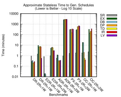
Figures 8 and 9 give the main results, which we step through in detail in the coming subsections; we describe the most important metrics here.


We call a specific combination of scheduler, actor system, and harness a configuration. Each schedule leads to a history of invocations and responses. We say a history is unique if, for a given configuration, no other history records the same events/entries (invocations and responses) in the same order with the same arguments, senders, receivers, and return values. That is, they are only chronologically unique. So, there could be some histories deemed unique but they are repeated many times except for re-arrangements of some entries that do not reveal a violation; those independent receives that materialize to a history’s entries. A history is non-linearizable if it cannot be generated by a linearizable implementation of the ADT being checked (e.g. a linearizable register or a map).
For a given configuration we call the ratio of non-linearizable histories to unique histories that are produced () the quality of that configuration. A high quality means that this configuration produces many examples of bugs while avoiding the need to check a large number of histories.
Similarly, we call the ratio of unique histories produced to schedules explored () the progression of that configuration. Intuitively, a high progression rate means the scheduler of that configuration produces a diverse set of histories with little exploration.
Finally, we call the ratio of non-linearizable histories produced to the number of schedules explored () the precision of a configuration. A configuration with high precision finds bugs by exploring fewer schedules, avoiding wasted work in fruitless ones.
For faster reference, all the above symbols and benchmarks abbreviations and their descriptions are shown in Table 1, while the raw numbers for the benchmarks results are shown in Tables 2 through 11. Each two consecutive tables starting from Table 2 show results for the same benchmark but one for 3-receives and the other for 4-receives.
As we will show later, our results show that the short histories that our harnesses produce mean that history checking times are low. Ultimately, this means that for our harnesses, good progression is crucial and good quality of the discovered histories is less important.
We record two different times for schedule exploration. The default is the time to generate the schedules in a stateful manner; meaning, the scheduler keeps snapshots of the actor system’s state during scheduling. The second one is an approximation of a stateless exploration of the system. This is as if the system is restarted after generating each schedule and controllably reconstructs different schedules in different runs, visiting different states than previously visited by earlier schedules. The advantage is memory pressure reduction during exploration. However, the stateful approach is faster to the finish line (overall time) at the expense of capturing states (using more memory) and slower per-iteration compute time. The reason why the stateful schedulers are faster overall time is that the prefixes of schedules are not executed as often as in the stateless schedulers. So, that saves a lot of time for stateful schedulers.
For most systems, we can explore the most interesting cases with just a few agents, so we only use two agents to test all but the buggy register, for which we use three agents. This still has the possibility of producing all of the externally visible system/ADT behaviors. More complex protocols could require more agents to explore all behaviors; for example, agent join/leave in protocols like Chord could require more agents to ensure all internal behaviors are exercised during schedules generation. Our implementation, however, does not need more as we do not have leaving processes and/or dropped messaging; we only implement joining.
Finally, with enough agents and invocations these algorithms can run for exceedingly long periods of time. We terminate exploration after 50,000 schedules per-configuration and then check the resulting histories. This cutoff means schedulers may miss fruitful parts of the exploration, and we observed such situations. We tried to strike a balance in choosing this cutoff, but no single cutoff is likely to work well for all configurations.
Last, the specific benchmarks numbers are as follows. The Lines Of Code (LOCs) in each benchmark range from few hundred lines to around a thousand lines. The number of actions involved range from 6 to 9 actions, not counting the start action that starts the agent.
All bugs found are real bugs, and all of the benchmarks were buggy (both linearizability and other bugs) before we debugged them. We kept all previous iterations of them as well in the repository 21. All of the benchmarking was done on the same machine, with each scheduler being single threaded. The specs of the machine are the following: Dual 3.5 GHz Intel XEON E5-2690 v3, 192GB DDR4 ECC, HP Z840 workstation.
A final note, we stressed tested IRed on the heaviest (buggy) implementation we have, namely the ADR register, for over 203 hrs monitoring it using VisualVM profiler and took notes of 20-25% of non-blocking single threaded CPU usage, 0% of Garbage Collector (GC) CPU usage all the time, and 4 GB of average use of heap memory and a max and min of 5 GB and 3 GB, respectively.
4.8 Results and Analysis
Figures 8 and 9 show the results of running the benchmarks across all of the configurations we described. We work through several dimensions of the table to highlight the key insights from the results.
4.8.1 Low History Checking Times
In virtually all cases, configurations avoid an explosion of runtime in checking histories using the exponential WGL algorithm (). Some of the configurations produce several unique histories (, Figure 8c), but since the harness is constrained to just a handful of invocations, checking all of them is still nearly instantaneous ( 1 second). Hence, though we were worried the complexity of checking histories would be problematic (poor quality), the explosion in schedulers state space seems to be a more serious issue (poor progression) (Figure 8a and 9a).
This suggests, just as in conventional model checking, smarter pruning or direction of scheduling is more important in finding bugs than reducing history checking time. This also reinforces our decision to focus our efforts on improving schedulers for linearizability checking rather than focusing on improving linearizability checking itself as others have done 14.
4.8.2 Systematic Random
The Systematic Random scheduler is ineffective in finding bugs (Figure 8b). It progresses well, and it produces many unique histories quickly (Figure 8d). However, even after doubling its cutoff to let it explore more schedules, it still finds only one bug in one configuration (the second harness of Open Chord), where other approaches find many more.
Coupled with the previous conclusion, this suggests that simply generating more histories alone is not sufficient to find bugs. This also suggests that any approach that simply tries to maximize “coverage” in the space of schedules or in the space of histories is not likely to yield bugs unless it is efficient enough to provide near-full coverage, which is unlikely due to the exponential explosion of exploration space.
4.8.3 Exhaustive and Delay-Bounded Performance
Exhaustive DFS (EX) and Delay-Bounded (DB) perform similarly in most cases and metrics, even though DB uses some bounded randomness. By delaying events, DB reorders the space of schedules, but without a cutoff, EX eventually explores the same schedules in a different order. So, DB’s limited randomness does little to change the set of schedules explored.
Both approaches do well at finding bugs with the first harness (2r+1w). In the other harness (2r+2w), they hit the cutoff rather quickly (Figure 8a), which indicates they generated too many fruitless schedules from the state space. This is reflected in their poor precision (, Figure 8f) and progression (, Figure 8d) ratios. If we removed the cutoff, they will find bugs in the second benchmark but only after generating large numbers of uninteresting schedules, which indicates they are not effective exploring larger state spaces.
An important observation is that chronological uniqueness of histories (involved in many measures), indicated by an asterisk ‘*’ in graphs of Figures 8 and 9) causes an issue. It causes redundancy in the counts of unique histories particularly so for schedulers exploring more redundant schedules (e.g. SR and DB). It amplifies the illusion of their effectiveness in generating more unique histories. The following is the list of all schedulers, ordered from most to least affected by this issue: SR, DB, EX, DP, TD, IR, LV. As we go from left to right in that list, the less amplification effect we get because there are fewer repeated chronologically unique histories; hence, the more credible the measures are of that specific scheduler. LiViola is the best due to being the least redundant. Unique histories it produced tended to have the most diversity among all. Even with this diversity, in Open Chord benchmarks, for example, LV produced four non-linearizable histories out of 17 unique histories on the smaller harness. When we cross-checked them with the larger harness we saw that they are the same history (i.e. the same exact bug), shown in Figure 7, and explained by the schedule shown in Listing 1. Note that the other write call of the second harness is on a different key (); hence, not shown, since it does not affect LV. However, it does affect all others’ results. If the related invocation and response are placed at the end of the history, one can imagine how many internal schedules that can be repeating the bug before it.
Another example on the other (most affected) extreme in Open Chord benchmarks, DB produces 3,557 unique histories and that reduce to 357 buggy ones while EX (which covers the same exhaustive state space), produces 325 unique histories that reduce to 15 buggy histories. None of them is more exhaustive than the other but DB is more repetitive than EX. The reason behind this is when the bug happens to be closer to the root of the exploration tree and the scheduler is interleaving things closer to leaves, the prefix containing the bug repeats as many times as the leaves. That has an amplification effect on bugs reported especially when the later interleavings after the prefix result in more chronologically unique histories.
4.8.4 DPOR, TransDPOR, and IRed Performance
In the distributed register, the three algorithms DPOR, TransDPOR, and IRed did better than EX and DB on both harnesses. DPOR, however, did slightly less favorably than TD and IR in terms of timing. The latter two did exactly the same. Otherwise, IR did not show any improvements over TD because this implementation is strongly causally consistent; hence, IR does not get an advantage over TD’s over-approximation of the root enabler. So, TD represents the worst-case scenario for IR.
In the second benchmark, DP and TD did mostly the same except for few differences on the 3 invocation test. DP produced fewer quality unique histories to catch bugs as indicated by , and it is less precise as indicated by than TD. However, results show it is more precise than IR. This is tempered by what we mentioned regarding repetitive chronological uniqueness of histories. TD was significantly faster at making progress towards unique schedules than DP. As for IR in the second benchmark, precision, quality and progression are slightly less than TD, but TD is more repetitive.
4.8.5 LiViola vs IRed Performance
LV performance numbers should have been exactly like IR’s on the register benchmarks, since they are one-key stores. LV enables developers to tweak the harness with interleaving exclusions (within the constraints we mentioned in §4.1 to assure soundness) to indicate which messages are the focus on during exploration (i.e. potentially interfere) which lead to significant improvements. It explores only 88 schedules in comparison to the second highest runners’ (IR and TD) 2,906 on the smaller harness, and does not approach the cutoff on the 4-invocations test, at 7,236 schedules. Meanwhile, IRed ran for over 203 hrs and still never terminated. However, developers should practice caution using this feature as we will see why in the next benchmark.
In the second benchmark, IR and LV were the best of the algorithms, too. They performed similarly except LV scored significantly better but were 2 seconds slower. In the third benchmark, LV performance was the worst-case scenario showing exact statistics as IR. Note that on the buggy version of this third (not shown here), when we tweaked the harness aggressively, LV outperformed all others by a large margin in the first harness. However, for the second test, it missed all bugs and prematurely terminated at a bit over 10K schedules stating it did not find bugs; when it should not miss bugs. So, we reverted these tweaks and passed a plain harness, i.e. with no tweaks, and re-run the experiments, shown in the Figures 8 and 9. This is an example of why developers are to practice caution when tweaking the harness while still conforming to the criteria presented in §4.1. The reader is encouraged to look at the rest of the numbers in tables in Appendix A for raw numbers, the best results we observed are for Open Chord.
4.9 Limitations
The model still has a limitation in conditionals e.g. If and While statements, in order to enable more sophisticated static and dynamic analyses such as symbolic execution. Another limitation, related to LiViola, stems from invisibility of where a certain key for a receive lies inside the message payload. That can happen when the key location is only determined later during runtime, by users specifying a wildcard location in the harness. If LV can not ascertain keys of different receives may conflict, it conservatively interleaves them not to hinder coverage. That, in turn, can compound rather quickly leading to the classic state space explosion problem but upper bounded by IRed’s state space.
The solution to the first limitation that relates to conditionals is to add a field that holds an Abstract Syntax Tree (AST), generated by scalameta 50 quasi-quotes, of the functional style conditions. That is for some analyses such as symbolic execution to be able to determine the satisfiability of certain path conditions 111111A path condition is the set of control-flow statement’s conditions, e.g. an if or while statements, when satisfied (or not), the scheduler can force the execution (or not to execute) of code blocks in the program along that path, i.e. their code blocks, across said statements..
One solution to the second limitation is to provide a function to be executed by LV each time to determine the location of targeted keys/variables based on information available during runtime. That, however, will require some, not many, modifications to LiViola to enable such feature.
4.10 Discussion
In this section we discuss few aspects regarding when our algorithms would be most effective at catching bugs, a comparison to the modern commonly used technique of concolic execution121212Symbolic execution paired with runtime partial runs to fulfill unknown information during static time but that are known only during dynamic/runtime time., and we end the discussion by some static and dynamic frameworks that can be integrated with ours to achieve more analyses.
We rely on the classification of bugs mentioned in 51 to comment the effectiveness of our technique at catching said bugs. Lopez et. al. 51 describe the following classes of actor-specific bugs that, in turn, are sub categorized further:
-
•
Lack of Progress: which includes communication deadlocks (two or more actors are blocked forever waiting for each other to do something), behavioral deadlocks (two or more actors waiting for a message to make progress, i.e. a message is never sent to allow for progress), live locks (similar to a deadlock but while involved actor’s states are changing but without making progress).
-
•
Message Protocol Violation: message order violation (where two or more actors exchange messages in a way violating the intended protocol), bad message interleaving (happens when a message is processed between the processing of two messages that are intended to be processed one after another), memory inconsistency (when different actors have different view of a conceptually shared resource).
Our algorithms address, and catches bugs most effectively, in the second class i.e. message protocol violations. On the other hand, our algorithms will exhibit communication deadlocks, behavioral deadlocks, and/or live locks, in the case of lack of progress class of bugs. Assuming we have implemented algorithms for catching the first class’ bugs, we would use these algorithms to first detect and remove that class of bugs. Only then, when the implementation is free from said bugs, we would use algorithms presented in this work. Our framework does not limit the ability from developing algorithms targeting lack of progress class of bugs. It, actually, has facilities to ease that task, by making it explicit which statements do block and whether it is blocking on external communication (e.g. a blocking get on a future, or a timed blocking statement on a future), and these blocking statements and constructs (a future) allow for the entire gradient of synchrony and asynchrony in communication and behavioral deadlocks detection. The snapshotting feature, of the entire global state of the distributed system, of our framework allows for detecting the lack of progress in the case of a live lock.
Symbolic execution 52, 53, and concolic testing 54, 55 would be a natural extension of our work, as mentioned in §4.9. It is a more advanced technique that incorporates Satisfiability Modulo Theory (SMT) solvers 56, 57, 58, 59 (or theorem provers) to determine a model that strictly follows a certain execution path. The set of conditions that forces that path is called a path condition. The conditions of control flow statements, such as an if or a while statement, are formulated as an SMT query to find a model to force that execution path in the code. This technique is more effective and more scalable than any of the DPOR methods used in this work. It provides more coverage, better performance, and more precision at targeting a certain criteria or code blocks. It enables more checks to be done on more involved implementations more effectively. Some of the bugs to target with concolic execution includes, but not limited to, dead code detection, deadlock detection, data races, termination, among other things. In other words, concolic execution is unmistakingly superior to all techniques presented in this paper. For example, instead of enumerating many equivalent schedules as in some of the algorithms in this work, a concolic tester can systematically target mostly unique schedules without the need to enumerate many of them. Once symbolic execution is enabled in our framework, it would be quiet interesting to implement a concolic algorithm to empirically compare it (both performance, precision, scalability) to our algorithms. That being said, while our technique only reports real bugs, symbolic execution might report false alarms and can be spurious, i.e. report the same/related bug many times. That is, when a bug falls on the start of a path condition, then all branches starting with the prefix of that path condition would lead to report that same bug, as many times. For concolic testing, this can be reduced/eliminated by synthesizing a representative test of that specific bug, running the test, and making sure if the bug actually manifests in the actual run. Symbolic execution may suffer the limitations of an SMT in case the path condition is too long having many conditions, conditions along the path have non-linear arithmetic, the path conditions involves cryptographic functions, or simply the path conditions involves some computation outside of an SMT solver’s capabilities. Still, more than one SMT solver can be mixed to complement each other’s strengths. In case some of the said limitations are still a limiting factor of symbolic executions, they can be overcome with concolic testing. The parts that are easy for an SMT solver (or a theorem prover) to figure out would still be solved symbolically; along with inputs that lead to that part of the code and that was determined by solving the constraints of that path condition(s). The parts that limits symbolic execution are to be test-ran (the concrete part of concolic) by the concolic tester, and hence the name concolic for CONCrete and symbOLIC. That enables the concolic tester to overcome the limitations of the symbolic execution and make progress towards corner cases that are hard to hit otherwise. Hitting the hard corner cases is a weakness for all algorithms of this paper as the input to the systems’ implementations (and through the scheduler) is done by the user, rather than a symbolic executor.
Hence, we made sure that only the very advanced analyses may need to call into external static and/or dynamic frameworks to analyze the model or augment the operation of algorithms/schedulers. The model composes actors/agents from a local state (a mapping construct with garbage collection that models the variables to values mapping in the scope), an activation frame stack (for function calls statement types with each activation frame having a LocalState object), and a mapping from message received to actions to be performed. There are other features but to simplify the overview for the reader, we omit those. The action is nothing but nested sequences of statement types. Each statement type wraps an actual statement in the form of a function to call and contains all the meta data a static/dynamic analyzing algorithm needs to access. All of the above is extensible, i.e. if more meta data were needed for a certain advanced algorithm the user definitely can extend those and add more meta data (i.e. fields/attributes to that class). Analyzing nested lists of statements, we think, is simple enough not to involve any other framework for the majority of tasks but still can be if the user chooses to. Similarly, algorithms and their auxiliary methods are all defined and ready to be used131313We highly encourage the reader to read the operational semantics of DS2 32 to realize and appreciate the capabilities there in. A simpler model paper for an overview is in 33. However, we understand for example that a more advanced user (or formal methods expert) would want to use e.g. SMTs that have Java/Scala APIs in their schedules/algorithms. That is possible, and there is nothing to interfere with their desire to involve static and/or dynamic analysis frameworks/tools. An example we tried before is to diagram the message flow from between actors using Graphviz 60 via Graph4s 61, similar to what was mentioned as MFG (message flow graphs) in Shian Li et al work 62. Similarly, we visualized the states for a sample run of several of the algorithms, e.g. WGL, while we were at the debugging stages of these algorithms. We took a look at the Backwards Symbolic Execution (BSE) by Shian Li et al 62 and we do not see any thing preventing the integration of such an advanced form of symbolic execution. The snapshot feature of DS2 definitely enables going back and forth in time without limits while exploring the subject distributed systems written in its model (a simple and extensible domain specific sanguage - DSL - as mentioned earlier). As a matter of fact, multiple more complex tools can be integrated into one scheduler and they can hand-off saved states to each other to do different exploration techniques in one algorithm; hence, forming a collection of the strengths of each collaboratively. That is, the algorithm can save the state of the system, using DS2’s lightweight snapshot feature, then BSE can do some kind of symbolic execution and after that returning the results. At this point, another snapshot can be taken, then either of these snapshots given to another algorithm to do another kind of analysis on the system, taking another snapshot after done and reporting back and so on. There is literally no limit but the host physical limits (e.g. amount of memory) on which that system is analyzed. After all, BSE, MFG, and DS2 all define formal operational semantics by which they can be more intimately integrated.
5 Related Work
In this section we taxonomize several related works. Covering both linearizability, model checking, tracing, monitoring, verification, proofs, …etc.
Linearizability. Linearizability has long been presented and extensively studied in literature; from the decision procedure perspective (checking) in the original paper by Herlihy 13, Jeanette Wing and Gong 15, and in WG Lowe 45. Testing for Linearizability 63 developed and evaluated five algorithms for randomly testing concurrent data types for linearizability violations, four of which are new. Also, four of which are generic while one is specific to concurrent queues. Winter et al. 64 derive an approach based on the instruction re-ordering rules for weak-memory models hardware in order to enable the re-use of existing methods and tool support for linearizability checking. Specifically, they target programs running on TSO (Total Store Order) and XC (Relaxed Consistency - cache coherence model) weak memory models. Ozkan et al. 65 show that linearizability of a history is often witnessed/realized by a schedule that re-orders small number of operations (), prioritizing schedules with fewer operations first in the exploration. The algorithm characterizes families of schedules of certain length of operations (depth) that is guaranteed to cover all linearizability witnesses of that depth. In our work, we experimented with minimal invocations that allow the subject systems to exhibit all externally observable behaviors, namely two and three invocations. In recent years, Kyle Kingsbury the author of Jepsen 12, came up with a new library, called Elle 66, to analyze histories produced by the former in order to find consistency violations. It is a sound framework, but since some information may be missing from observed histories, not complete. Hadzilacos et al 67 invalidate a conjuncture that says if we replace an atomic object in an algorithm by another object that is linearizable, then the algorithm stays the same. One result of their work is that in randomized algorithms, when an atomic register was replaced by a linearizable one, it lead to violating the all-important property of termination with probability of 1. Hence, they propose a new stronger type of register linearizability called write strong-linearizability. It is strictly stronger than (plain) linearizability but strictly weaker than strong linearizability and it fixes the above. Bashari et al 68 states that in most algorithms n-processes updating different array locations in an array, a scan would produce a linearizable snapshot of the array. However, that requires a scan operation of the array. They came up with an approach to produce such array in a constant time complexity, and a observe and update operations, hence improving the performance. Sela et al 69 point out and provide an amendment to the original linearizability paper. The typo addresses the issue of handling invocations in volatile memory setups and hence it was significant.
Model Checking. Doolan et al. 70 studied the SPIN 71 model checker algorithm to understand the scalability issues in an effort to scale automatic linearizability checking and without manual specification of linearization points by the users. They also provide proof-of-concept implementation. Our work does that, also, and without manual specification of linearization points due to the atomic nature of the actor-model actions in our model. However, our algorithms are generic and can be applied to other problems that can be mapped to race conditions checking and without the need to write a separate model e.g. in Promela 72 (the implementation is the model). Vechev et al. 73 provide an experience report summarizing first experience with model checking linearizability. It was the first work to achieve that with non-fixed linearization points. Zhang et al. 74 employed model checking, partial order reduction, and symmetry between threads to reduce the state space to model check for linearizability. SAMC! 38 is a model checking tool targeting message-reordering, crashes of processes, and reboots deep bugs in distributed systems. It requires semantic annotation to reduce the systematic exploration of state space. Our tool-chain is similar in the sense that it uses the operational semantics to reduce the search space but without the need for users to manually enter annotations. Chong et al 75 describes a style of applying symbolic model checking developed over the course of four years at Amazon Web Services (AWS), lists lessons learned, and provides a list of proofs developed throughout their experience developing for Amazon’s AWS.
Tracing. Çirisci er al. 76 propose an approach that points the root-cause of linearizability violations in the form of code blocks whose atomicity is required to restore linearizability. That is, the problem can be reduced to identifying minimal root causes of conflict serializability violation in an error trace combined with a heuristic to find out which is the more likely cause of the linearizability violation. Zhang et al. 77 present a tool called CGVT to build a small test case that is sufficient enough for reproducing a linearizability fault. Based on a possibly long history that was deemed non-linearizable, the tool locates the offending operations and synthesizes a minimal test-case for further investigation. Zhang et al. 78 provide a better approach than CGTV by coming up with what is called critical data race sequence (CDRS) that side steps the shortcoming of the coarse-grained interleaving when linearizability is violated. The new fine-grained trace model helps in better localizing the linearizability violations using labeled-tree model of program executions. They implement and evaluate their approach in another (subsequent to CGTV) tool called FGVT (Fine-Grained-Veri-Trace).
Quasi Linearizability. Zhang et al. 79 on runtime checking for quasi linearizability. This is a more relaxed form of linearizability. The authors of a tool called Inspect implemented a fully automatic approach using LLVM to detect and report real violation of quasi linearizability. Adhikari et al. 80 verify quantitative relaxation of quasi linearizability of an implementation model of the data structure. It is based on checking the refinement relation between the implementation and a specification model. They implement and evaluate their approach in a framework called PAT verification framework.
Fixing Linearizability. Liu et al. 81 address the problem of fixing non-linearizable composed operations such that they behave atomically in concurrent data structures. The algorithm (Flint) accepts a non-linearizable composed-operations on a map. Its output, if it succeeds at fixing the operations, is a linearizable composed operation that is equivalent to a sequential data structure execution. The effectiveness of the algorithm is 96% based on 48 incorrect input compositions.
Verification. Liang et al. 82 propose a program logic with a lightweight instrumentation mechanism which can verify algorithms with non-fixed linearization points. This work was evaluated on various classic algorithms some of which used in java.util.concurrent package. Bouajjani et al. 83 consider concurrent priority queues, fundamental to many multi-threaded applications such as task scheduling. It shows that verifying linearizability of such implementations can be reduced to control-state reachability. This result makes verifying said data-structures in the context of unbounded number of threads decidable.
Runtime Monitoring. Emmi et al. 84 leverage an observation about properties that admit polynomial-time (instead of exponential time) linearizability monitoring for certain concurrent collections data types, e.g. queues, sets, stacks, and maps. It uses these properties to reduce linearizability to Horn satisfiability. This work is the first in linearizability monitoring that is sound, complete, and tractable. Emmi et al. 85 identify an optimization for weak-consistency checking that relies on a minimal visibility relations that adhere to various constraints of the given criteria. Hence, saving time instead of exponential enumerations of possible visibility relations among the linearized operations. This, as the work before it, is a monitoring approach.
Proofs/Proving. Henzinger et al. 86 argue that the non-monolithic approaches based on linearization points (automatic or manual) are both complicated and do not scale well e.g. in optimistic updates. The work proposes a more modular alternative approach of checking linearizability of concurrent queue algorithms. Hence, reducing linearizability proofs of concurrent queues to four basic properties, each of which can be proven independently by simpler arguments. Sergey et al. 87 propose a uniform alternative to other approaches in the form of Hoare logic, which can explicitly capture the interference of threads in an auxiliary state. This work implements the mechanized proof methodology in a Coq-based tool and verifies some implementations with non-standard conditions of concurrency-aware linearizability, quiescent and quantitative quiescent consistency.
Compositionality of Linearizability. P-compositionality statically decomposes concurrent objects’ (ADTs’) histories based on different operations’ target keys into sub-histories (one per key) to check for linearizability 19. LiViola, our algorithm, was inspired by the latter but we applied this concept at the more critical scheduler level, as we found out later in the experiments. Scheduling. Recently, an approach that uses invariants and dynamic scheduling to achieve consistency-aware scheduling for weakly consistent geo-replicated data stores has been presented 88, evaluated, and found effective. It was implemented and evaluated in a model checker for Antidote DB 89.
Causality. Prior to that there was what is called Causal Linearizability 90. Given some constraints on the clients, a more generic causality checking can be achieved. The actor model (also our model) conforms to such constraint on a per-process (per actor) scheduled task. Maximum Causality Reduction 91 uses causality information on the trace level to reduce the state space to explore for TSO (Total Store Order) and PSO (Partial Store Order) to check for Sequential Consistency. Bita 7 is an algorithm used to generate causally-consistent schedules of receives.
Checking Histories for Linearizability Violations. As for the WGL algorithm implementations, there are several other than ours. A Go-implementation 92 that requires invariants input by users to the tool, and another CPP implementation 47 that works on already output traces exist. A similar tool-chain to ours, called Jepsen 93, 12, 94 (generates histories/traces) and its engine Knossos 95 (generates schedules) is widely used to check key-value stores linearizability, black box fuzzing. It needs significant amount of work from the user studying how the subject system works and then devises a test harness, which takes months of insightful work. It handles faults while our algorithms do not; although, they can if extended due to the model being readily prepared for simulating faults. LineUp 96, Microsoft Research’s primary C#/.NET concurrent objects tester, existed for a long time and it is effective at exposing concurrent data structures linearizability violations.
Fault Injection. Peter Alvaro’s work on lineage driven fault injection 97, consistency without borders 98, Automating Failure Testing Research At Internet Scale 99 was an inspiration in designing and steering our framework and its extensibility.
Runtime Scheduling. ARTful 100 is a model for user-defined schedulers targeting various high performance computing (HPC) systems. HPC systems, a specialized kind of distributed systems, usually experience some load balancing issues and this work allows users to regain control over wasted resources. Experiments in this work has been conducted on OpenMP 101 and Charm++ 102 runtime systems.
Specification Languages. Pluscal 103 is an algorithm language that is used to specify distributed systems. Users need to hand write models in this language to enable the runtime to check desired properties.
Learning Based Approaches. Mukherjee et al 104 developed a technique for controlled concurrency testing (CCT) using machine learning to address scale of the state space in concurrent programs interleavings. This work developed a framework, called QL, where they rely on Q-Learning algorithm to decide the next action to be explored. That, in turn, is influenced by the previously selected actions in the exploration. This work was benchmarked against a set of microbenchmarks, complex protocols, and production cloud services and performed well. In future works, we may employ similar techniques, i.e. machine learning, to compare against such algorithms. Another work, Marcén et al 105 tackled the integration problem for machine learning classifiers to augment model driven development (MDD) in two real industrial setups and it paid off. Our framework still does not have the synthesis functionality. However, we plan to explore this direction in future work since it showed encouraging results in many other setups e.g. github co-pilot as well.
6 Concluding Remarks
In this work, we used only four out of sixteen semantics rules our model provides, namely: Schedule, Consume, Send, and Message-Reordering. One can extend these algorithms and utilize them to address more problems. In the near future, we would like to add more benchmarks, schedulers and address more systems faults. In addition, we want to remove all model limitations to enable further static and/or dynamic introspection. Also, all our expectations we theorized were met and exceeded. However, there are still room to improve IRed and LiViola. Some heuristics that may yield these improvements include the following: 1) prioritizing longer causal-chains execution earlier in the exploration tree, and 2) introspection into code to produce longer causal chains that involve as many enabled receives as possible, and 3) the conflicting keys (in LiViola) can be viewed as program variables and hence it extends to other than key-value stores. After conducting this experiment, we realized that many concurrency bugs can reduce/mapped to race condition detection, e.g. LiViola and linearizability. Last, and foremost, we have learned the following lessons out of this work:
-
1.
Lesson 1: This work informed the fact that focusing on schedules pruning is more effective than focusing on improving linearizability checking itself.
-
2.
Lesson 2: Any approach that simply tries to maximize “coverage” in the spaces of schedules or histories is not likely to yield bugs unless it is efficient enough to provide near-full coverage
-
3.
Lesson 3: Chronological uniqueness of histories can mislead that worse algorithms perform better (being too repetitive amplifies the perception of finding more bugs by revealing the same bug/history more repetitively).
-
4.
Lesson 4: Layering complexity cleanly enables addressing more of it, more easily, and modularily. This is exemplified by using only 4 operational semantics rules, and future work adding more complexities using more semantics rules in future specialized schedulers.
Future Work. At the end, we would like to mention some of the potential future direction(s) for us. We find that implementing some of the termination detection algorithms by Dan Plyukhin et al 106, 107 interesting to show and test more of the capabilities of our framework.
Acknowledgments. We would like to thank Zvonimir Rakamaric for steering the work towards this fruitful direction, and the following who contributed significantly to the project: Heath French, Zepeng Zhao, Jarkko Savela, Anushree Singh.
NSF Funding. This work has been partially funded by both NSF grant CCF 1302449, CCF 1956106 and NSF grant CSR 1421726.
References
- 1 Akka. http://akka.io/, Retrieved May 3, 2016.
- 2 Erlang Programming Language. 2018. https://www.erlang.org/.
- 3 Bernstein PA, Bykov S, Geller A, Kliot G, Thelin J. Orleans: Distributed Virtual Actors for Programmability and Scalability. Tech. Rep. MSR-TR-2014-41, 2014.
- 4 Meiklejohn CS, Miller H, Alvaro P. PARTISAN: Scaling the Distributed Actor Runtime. In: USENIX Association; 2019; Renton, WA: 63–76.
- 5 Inside Fortnite’s Massive Data Analytics Pipeline. https://www.datanami.com/2018/07/31/inside-fortnites-massive-data-analytics-pipeline/, Retrieved May 5, 2020.
- 6 Who is using Orleans. https://dotnet.github.io/orleans/Community/Who-Is-Using-Orleans.html, Retrieved May 5, 2020.
- 7 Tasharofi S, Pradel M, Lin Y, Johnson R. Bita: Coverage-guided, automatic testing of actor programs. In: ; 2013: 114-124
- 8 Tasharofi S, Karmani RK, Lauterburg S, Legay A, Marinov D, Agha G. TransDPOR: A Novel Dynamic Partial-order Reduction Technique for Testing Actor Programs. In: FMOODS’12/FORTE’12. Springer-Verlag; 2012; Berlin, Heidelberg: 219–234
- 9 Lauterburg S, Karmani RK, Marinov D, Agha G. Basset: a tool for systematic testing of actor programs. In: Roman G, Hoek v. dA. , eds. Proceedings of the 18th ACM SIGSOFT International Symposium on Foundations of Software Engineering, 2010, Santa Fe, NM, USA, November 7-11, 2010ACM; 2010: 363–364
- 10 Wilcox JR, Woos D, Panchekha P, et al. Verdi: A Framework for Implementing and Formally Verifying Distributed Systems. ACM SIGPLAN Notices 2015; 50(6): 357–368. doi: 10.1145/2813885.2737958
- 11 Coq, Inria. https://coq.inria.fr/, Retrieved Feb 27, 2016.
- 12 Distributed Systems Safety Research. https://jepsen.io/, Retrieved Feb 27, 2018.
- 13 Herlihy MP, Wing JM. Linearizability: A Correctness Condition for Concurrent Objects. ACM Trans. Program. Lang. Syst. 1990; 12(3): 463–492. doi: 10.1145/78969.78972
- 14 Horn A, Kroening D. Faster linearizability checking via $P$-compositionality. CoRR 2015; abs/1504.00204.
- 15 Wing J, Gong C. Testing and Verifying Concurrent Objects. Journal of Parallel and Distributed Computing 1993; 17(1): 164 - 182. doi: https://doi.org/10.1006/jpdc.1993.1015
- 16 Ongaro D, Ousterhout J. In Search of an Understandable Consensus Algorithm. In: USENIX ATC’14. USENIX Association; 2014; Berkeley, CA, USA: 305–320.
- 17 Liskov B, Cowling J. Viewstamped replication revisited. 2012.
- 18 Lamport L. Paxos Made Simple. SIGACT News 2001; 32(4): 51–58.
- 19 Singh V, Neamtiu I, Gupta R. Proving Concurrent Data Structures Linearizable. In: ; 2016: 230-240
- 20 Flanagan C, Godefroid P. Dynamic Partial-Order Reduction for Model Checking Software. In: POPL ’05. Association for Computing Machinery; 2005; New York, NY, USA: 110–121
- 21 DS2 - Declarative Specification of Distributed Systems. https://gitlab.com/mohd_sm81/ds2, Retrieved Jan 20, 2021.
- 22 DeCandia G, Hastorun D, Jampani M, et al. Dynamo: Amazon’s Highly Available Key-value Store. SIGOPS Operating Systems Review 2007; 41(6): 205–220. doi: 10.1145/1323293.1294281
- 23 The Apache Software Foundation . Apache Cassandra. http://cassandra.apache.org/; .
- 24 Gifford DK. Weighted Voting for Replicated Data. In: SOSP ’79. Association for Computing Machinery; 1979; New York, NY, USA: 150–162
- 25 OpenChord Akka Implementation, in Java and Scala. https://bitbucket.org/onedash/akka-open-chord, Retrieved April 8, 2018.
- 26 OpenChord Akka Implementation, Scala only. https://github.com/allenfromu/Open-Chord-Scala, Retrieved April 8, 2018.
- 27 Zave P. How to Make Chord Correct (Using a Stable Base). CoRR 2015; abs/1502.06461.
- 28 Stoica I, Morris R, Karger D, Kaashoek MF, Balakrishnan H. Chord: A Scalable Peer-to-peer Lookup Service for Internet Applications. In: SIGCOMM ’01. ACM; 2001; New York, NY, USA: 149–160
- 29 Chandra TD, Griesemer R, Redstone J. Paxos Made Live: An Engineering Perspective. In: PODC ’07. ACM; 2007; New York, NY, USA: 398–407
- 30 Lamport L. The Part-time Parliament. ACM Transactions on Computer Systems 1998; 16(2).
- 31 Paxos Akka Implementation. https://github.com/allenfromu/Multi-Paxos-UDP, Retrieved April 8, 2018.
- 32 Al-Mahfoudh MS, Gopalakrishnan G, Stutsman R. Operational Semantics for the Rigorous Analysis of Distributed Systems. In: Rubin SH, Bouabana-Tebibel T. , eds. Quality Software Through Reuse and IntegrationSpringer International Publishing; 2018; Cham: 209–231.
- 33 Al-Mahfoudh M, Gopalakrishnan G, Stutsman R. Toward Rigorous Design of Domain-specific Distributed Systems. In: FormaliSE ’16. ACM; 2016; New York, NY, USA: 42–48
- 34 DS2 Official Website. 2016. http://formalverification.cs.utah.edu/ds2, Retrieved Jan 31, 2016.
- 35 Agha G. Actors: A Model of Concurrent Computation in Distributed Systems. PhD thesis. MIT, 1985.
- 36 Hewitt C, Bishop P, Steiger R. A Universal Modular ACTOR Formalism for Artificial Intelligence. In: IJCAI’73. Morgan Kaufmann Publishers Inc.; 1973; San Francisco, CA, USA: 235–245.
- 37 Actor Model - Wikipedia. https://en.wikipedia.org/wiki/Actor_model, Retrieved May 13, 2020.
- 38 Leesatapornwongsa T, Hao M, Joshi P, Lukman JF, Gunawi HS. SAMC: Semantic-aware Model Checking for Fast Discovery of Deep Bugs in Cloud Systems. In: OSDI’14. USENIX Association; 2014; Berkeley, CA, USA: 399–414.
- 39 Pavlo A, Jones EP, Zdonik S. On Predictive Modeling for Optimizing Transaction Execution in Parallel OLTP Systems. PVLDB 2011; 5: 85–96.
- 40 Jhala R, Majumdar R. Software Model Checking. ACM Computing Surveys 2009; 41(4): 21:1–21:54. doi: 10.1145/1592434.1592438
- 41 Yang J, Chen T, Wu M, et al. MODIST: Transparent Model Checking of Unmodified Distributed Systems. In: USENIX Association; 2009: 213–228.
- 42 Flanagan C, Godefroid P. Dynamic Partial-Order Reduction for Model Checking Software. SIGPLAN Not. 2005; 40(1): 110–121. doi: 10.1145/1047659.1040315
- 43 Nielsen B, Agha G. Semantics for an Actor-Based Real-Time Language. In: Naval Surface Warfare Center Dahlgren Division/IEEE (ed.) . , ed. Proceedings of the 4th International Workshop on Parallel and Distributed Real-Time Systems (WPDRTS), Honolulu, Hawaii, April 1995<Forlag uden navn>; 1995: 223–228. Semantics for an Actor-Based Real-Time Language ; Conference date: 19-05-2010.
- 44 Rebeca Modeling Language. https://rebeca-lang.org/, Retrieved Jun 9, 2022.
- 45 Lowe G. Testing for linearizability. Concurrency and Computation: Practice and Experience; 29(4): e3928. doi: 10.1002/cpe.3928
- 46 Emmi M, Qadeer S, Rakamaric Z. Delay-Bounded Scheduling. Tech. Rep. MSR-TR-2010-123, 2010.
- 47 Linearizability Checker. https://github.com/ahorn/linearizability-checker, Retrieved April 10, 2018.
- 48 Van Renesse R, Schiper N, Schneider FB. Vive la différence: Paxos vs. viewstamped replication vs. zab. IEEE Transactions on Dependable and Secure Computing 2014; 12(4): 472–484.
- 49 Junqueira FP, Reed BC, Serafini M. Zab: High-performance broadcast for primary-backup systems. In: ; 2011: 245-256
- 50 Scalameta - Library to read, analyze, transform and generate Scala programs. https://scalameta.org/, Retrieved Jan 20, 2021.
- 51 López C, Marr S, Mössenböck H, Gonzalez Boix E. A Study of Concurrency Bugs and Advanced Development Support for Actor-based Programs. 2017.
- 52 Symbolic Execution. https://en.wikipedia.org/wiki/Symbolic_execution, Retrieved Jun 19, 2022.
- 53 Li P, Li G, Gopalakrishnan G. Practical Symbolic Race Checking of GPU Programs. .
- 54 Concolic Testing. https://en.wikipedia.org/wiki/Concolic_testing, Retrieved Jun 19, 2022.
- 55 Sen K, Agha G. Automated Systematic Testing of Open Distributed Programs. In: Baresi L, Heckel R. , eds. Fundamental Approaches to Software EngineeringSpringer Berlin Heidelberg; 2006; Berlin, Heidelberg: 339–356.
- 56 Z3 SMT Sovler. https://github.com/Z3Prover/z3, Retrieved April 10, 2018.
- 57 SAT4J. http://www.sat4j.org/, Retrieved April 10, 2018.
- 58 CVC5. https://cvc5.github.io/, Retrieved Jun 20, 2022.
- 59 Satisfiability modulo theories. https://github.com/Z3Prover/z3, Retrieved Jun 20, 2022.
- 60 Graphviz. https://graphviz.org/, Retrieved Jun 22, 2022.
- 61 Graph for Scala. Retrieved Jan 31, 2016.
- 62 Li S, Hariri F, Agha G. Targeted test generation for actor systems. In: Millstein T. , ed. 32nd European Conference on Object-Oriented Programming, ECOOP 2018Leibniz International Proceedings in Informatics, LIPIcs. Schloss Dagstuhl- Leibniz-Zentrum fur Informatik GmbH, Dagstuhl Publishing; 2018
- 63 Lowe G. Testing for linearizability. Concurrency and Computation: Practice and Experience 2017; 29(4): e3928. e3928 cpe.3928doi: https://doi.org/10.1002/cpe.3928
- 64 Winter K, Smith G, Derrick J. Observational Models for Linearizability Checking on Weak Memory Models. In: ; 2018: 100-107
- 65 Ozkan BK, Majumdar R, Niksic F. Checking Linearizability Using Hitting Families. In: PPoPP ’19. Association for Computing Machinery; 2019; New York, NY, USA: 366–377
- 66 Kingsbury K. Elle: Finding Isolation Violations in Real-World Databases. In: PODC’21. Association for Computing Machinery; 2021; New York, NY, USA: 7
- 67 Hadzilacos V, Hu X, Toueg S. On Register Linearizability and Termination. In: PODC’21. Association for Computing Machinery; 2021; New York, NY, USA: 521–531
- 68 Bashari B, Woelfel P. An Efficient Adaptive Partial Snapshot Implementation. In: PODC’21. Association for Computing Machinery; 2021; New York, NY, USA: 545–555
- 69 Sela G, Herlihy M, Petrank E. Brief Announcement: Linearizability: A Typo. In: PODC’21. Association for Computing Machinery; 2021; New York, NY, USA: 561–564
- 70 Doolan P, Smith G, Zhang C, Krishnan P. Improving the Scalability of Automatic Linearizability Checking in SPIN. In: Duan Z, Ong L. , eds. Formal Methods and Software EngineeringSpringer International Publishing; 2017; Cham: 105–121.
- 71 Holzmann GJ. Logic Verification of ANSI-C Code with SPIN. In: . 1885 of Lecture Notes in Computer Science. Springer; 2000: 131–147.
- 72 Spin. http://spinroot.com/spin/whatispin.html, Retrieved Feb 27, 2016.
- 73 Vechev M, Yahav E, Yorsh G. Experience with Model Checking Linearizability. In: Păsăreanu CS. , ed. Model Checking SoftwareSpringer Berlin Heidelberg; 2009; Berlin, Heidelberg: 261–278.
- 74 Zhang S. Scalable automatic linearizability checking. In: IEEE Computer Society; 2011; Los Alamitos, CA, USA: 1185-1187
- 75 Chong N, Cook B, Eidelman J, et al. Code-level model checking in the software development workflow at Amazon Web Services. Software: Practice and Experience 2021; 51(4): 772-797. doi: https://doi.org/10.1002/spe.2949
- 76 Çirisci B, Enea C, Farzan A, Mutluergil SO. Root Causing Linearizability Violations. In: Lahiri SK, Wang C. , eds. Computer Aided VerificationSpringer International Publishing; 2020; Cham: 350–375.
- 77 Zhang Z, Wu P, Zhang Y. Localization of Linearizability Faults on the Coarse-Grained Level. International Journal of Software Engineering and Knowledge Engineering 2017; 27(09n10): 1483-1505. doi: 10.1142/S0218194017400071
- 78 Chen Y, Zhang Z, Wu P, Zhang Y. Interleaving-Tree Based Fine-Grained Linearizability Fault Localization. In: Feng X, Müller-Olm M, Yang Z. , eds. Dependable Software Engineering. Theories, Tools, and ApplicationsSpringer International Publishing; 2018; Cham: 108–126.
- 79 Lu Zhang , Chattopadhyay A, Wang C. Round-up: Runtime checking quasi linearizability of concurrent data structures. In: ; 2013: 4-14
- 80 Adhikari K, Street J, Wang C, Liu Y, Zhang S. Verifying a Quantitative Relaxation of Linearizability via Refinement. In: Bartocci E, Ramakrishnan CR. , eds. Model Checking SoftwareSpringer Berlin Heidelberg; 2013; Berlin, Heidelberg: 24–42.
- 81 Liu P, Tripp O, Zhang X. Flint: Fixing Linearizability Violations. SIGPLAN Not. 2014; 49(10): 543–560. doi: 10.1145/2714064.2660217
- 82 Liang H, Feng X. Modular Verification of Linearizability with Non-Fixed Linearization Points. SIGPLAN Not. 2013; 48(6): 459–470. doi: 10.1145/2499370.2462189
- 83 Bouajjani A, Enea C, Wang C. Checking Linearizability of Concurrent Priority Queues. CoRR 2017; abs/1707.00639.
- 84 Emmi M, Enea C. Sound, Complete, and Tractable Linearizability Monitoring for Concurrent Collections. Proc. ACM Program. Lang. 2017; 2(POPL). doi: 10.1145/3158113
- 85 Emmi M, Enea C. Monitoring Weak Consistency. In: Chockler H, Weissenbacher G. , eds. Computer Aided VerificationSpringer International Publishing; 2018; Cham: 487–506.
- 86 Henzinger TA, Sezgin A, Vafeiadis V. Aspect-Oriented Linearizability Proofs. In: D’Argenio PR, Melgratti H. , eds. CONCUR 2013 – Concurrency TheorySpringer Berlin Heidelberg; 2013; Berlin, Heidelberg: 242–256.
- 87 Sergey I, Nanevski A, Banerjee A, Delbianco GA. Hoare-Style Specifications as Correctness Conditions for Non-Linearizable Concurrent Objects. In: OOPSLA 2016. Association for Computing Machinery; 2016; New York, NY, USA: 92–110
- 88 Dabaghchian M, Rakamaric Z, Ozkan BK, Mutlu E, Tasiran S. Consistency-Aware Scheduling for Weakly Consistent Programs. SIGSOFT Softw. Eng. Notes 2018; 42(4): 1–5. doi: 10.1145/3149485.3149493
- 89 Shapiro M, Bieniusa A, Preguiça N, Balegas V, Meiklejohn C. Just-Right Consistency: reconciling availability and safety. 2018.
- 90 Doherty S, Derrick J. Linearizability and Causality. In: De Nicola R, Kühn E. , eds. Software Engineering and Formal MethodsSpringer International Publishing; 2016; Cham: 45–60.
- 91 Huang S, Huang J. Maximal Causality Reduction for TSO and PSO. SIGPLAN Not. 2016; 51(10): 447–461. doi: 10.1145/3022671.2984025
- 92 Porcupine. https://github.com/anishathalye/porcupine, Retrieved April 10, 2018.
- 93 Jepsen. https://aphyr.com/tags/jepsen, Retrieved April 7, 2018.
- 94 Jepsen. https://github.com/jepsen-io/jepsen, Retrieved April 10, 2018.
- 95 Knossos: Verifies the linearizability of experimentally accessible histories.. https://github.com/jepsen-io/knossos, Retrieved Apr 17, 2018.
- 96 Burckhardt C, Musuvathi M, Tan R. Line-up: A Complete and Automatic Linearizability Checker. SIGPLAN Not. 2010; 45(6): 330–340. doi: 10.1145/1809028.1806634
- 97 Alvaro P, Rosen J, Hellerstein JM. Lineage-driven Fault Injection. In: SIGMOD ’15. ACM; 2015; New York, NY, USA: 331–346
- 98 Alvaro P, Bailis P, Conway N, Hellerstein JM. Consistency Without Borders. In: SOCC ’13. ACM; 2013; New York, NY, USA: 23:1–23:10
- 99 Alvaro P, Andrus K, Sanden C, Rosenthal C, Basiri A, Hochstein L. Automating Failure Testing Research at Internet Scale. In: SoCC ’16. ACM; 2016; New York, NY, USA: 17–28
- 100 Santana A, Freitas V, Castro M, Pilla LL, Méhaut JF. ARTful: A model for user-defined schedulers targeting multiple high-performance computing runtime systems. Software: Practice and Experience 2021; 51(7): 1622-1638. doi: https://doi.org/10.1002/spe.2977
- 101 OpenMP. https://www.openmp.org/, Retrieved Jun 22, 2022.
- 102 Charm++. https://charmplusplus.org/, Retrieved Jun 22, 2022.
- 103 Lamport L. The PlusCal Algorithm Language. Theoretical Aspects of Computing-ICTAC 2009, Martin Leucker and Carroll Morgan editors. Lecture Notes in Computer Science, number 5684, 36-60. 2009.
- 104 Mukherjee S, Deligiannis P, Biswas A, Lal A. Learning-Based Controlled Concurrency Testing. Proc. ACM Program. Lang. 2020; 4(OOPSLA). doi: 10.1145/3428298
- 105 Marcén AC, Pérez F, Pastor O, Cetina C. Evaluating the benefits of empowering model-driven development with a machine learning classifier. Software: Practice and Experience 2022; 52(11): 2439-2455. doi: https://doi.org/10.1002/spe.3133
- 106 Plyukhin D, Agha G. Scalable Termination Detection for Distributed Actor Systems. In: Konnov I, Kovács L. , eds. 31st International Conference on Concurrency Theory, CONCUR 2020, September 1-4, 2020, Vienna, Austria (Virtual Conference). 171 of LIPIcs. Schloss Dagstuhl - Leibniz-Zentrum für Informatik; 2020: 11:1–11:23
- 107 Plyukhin D, Agha G. A Scalable Algorithm for Decentralized Actor Termination Detection. Log. Methods Comput. Sci. 2022; 18(1). doi: 10.46298/lmcs-18(1:39)2022
Appendix A Raw Data for the Benchmarks
| Symbol | Meaning |
| EX | Exhaustive Scheduler |
| SR | Systematic Random Scheduler |
| DB | Delay-Bounded Scheduler |
| DP | DPOR - Dynamic Partial Order Reducing Scheduler |
| TD | TransDPOR - Transitive DPOR |
| IR | IRed Scheduler - generic precise causality tracking scheduler |
| LV | LiViola - specialized Linearizability Violation Scheduler, and transitive race scheduler |
| #Agents | Number of agents in the system |
| #Rtry | Number of retries per request |
| Qrm | Number of agents forming to form a quorum in the system |
| #Inv | Number of invocations, 2R+1W means 2 reads and 1 write |
| #S | Number of schedules |
| #IH | Number of incomplete histories |
| #UH | Number of chronologically unique histories |
| #NL | Number of Non-Linearizable unique histories |
| NL/UH | Number of Non-Linearizable unique histories to total number of unique histories ratio, or the quality |
| UH/S | Number of unique histories to the number of schedules ratio, or the progression |
| NL/S | Number of Non-Linearizable unique histories to the number of schedules ratio, or the precision |
| TS | The time spent by the scheduler to generate all schedules |
| ST | The approximate time if the scheduler is to produce the same schedules but statelessly |
| TC | The time spent to check all unique histories in the configuration |
| TT | The total time spent to both generate schedules and check all unique histories, |
| #HF | Number of histories before catching the first buggy (non-linearizable) history |
| TF | The time to hit the first buggy (non-linearizable) history |
| #Inv. | 2R+1W | |||||||
| Alg. | EX | SR | DB | DP | TD | IR | LV | |
|
Distributed Register
#Agents = 2 #Rtry = 3 Qrm = 2 |
#S | 4,200 | 100K | 4,200 | 2,984 | 2,906 | 2,906 | 88 |
| #IH | 4,195 | 0 | 4,195 | 2,979 | 2,901 | 2,901 | 83 | |
| #UH | 37 | 26 | 37 | 37 | 37 | 37 | 22 | |
| #NL | 0 | 0 | 0 | 0 | 0 | 0 | 0 | |
| NL/UH | 0.0 % | 0.0% | 0.0% | 0.0% | 0.0% | 0.0% | 0.0% | |
| UH/S | 0.88% | 0.03% | 0.88% | 1.24% | 1.27% | 1.27% | 25.0% | |
| NL/S | 0.0% | 0.0% | 0.0% | 0.0% | 0.0% | 0.0% | 0.0% | |
| TS | 0:06 | 4:48 | 0:06 | 0:05 | 0:05 | 0:04 | 0:00 | |
| ST | 0:18 | 1:52 | 0:21 | 0:12 | 0:13 | 0:17 | 0:00 | |
| TC | 0:00 | 0:00 | 0:00 | 0:00 | 0:00 | 0:00 | 0:00 | |
| TT | 0:06 | 4:48 | 0:06 | 0:05 | 0:05 | 0:04 | 0:00 | |
| #HF | - | - | - | - | - | - | - | |
| TF | 0:00 | 0:00 | 0:00 | 0:00 | 0:00 | 0:00 | 0:00 | |
| #Inv. | 2R+2W | |||||||
| Alg. | EX | SR | DB | DP | TD | IR | LV | |
|
Distributed Register
#Agents = 2 #Rtry = 3 Qrm = 2 |
#S | 50K | 100K | 50K | 50K | 50K | 50K | 7,236 |
| #IH | 50K | 100K | 50K | 50K | 50K | 50K | 7,236 | |
| #UH | 8 | 91 | 8 | 8 | 8 | 8 | 147 | |
| #NL | 0 | 0 | 0 | 0 | 0 | 0 | 0 | |
| NL/UH | 0.0% | 0.0% | 0.0% | 0.0% | 0.0% | 0.0% | 0.0% | |
| UH/S | 0.02% | 0.09% | 0.02% | 0.02% | 0.02% | 0.02% | 2.03% | |
| NL/S | 0.0% | 0.0% | 0.0% | 0.0% | 0.0% | 0.0% | 0.0% | |
| TS | 1:27 | 5:49 | 1:22 | 1:36 | 1:34 | 1:34 | 0:09 | |
| ST | 9:27 | 2:55 | 6:27 | 7:09 | 7:42 | 7:05 | 0:34 | |
| TC | 0:00 | 0:00 | 0:00 | 0:00 | 0:00 | 0:00 | 0:00 | |
| TT | 1:27 | 5:49 | 1:22 | 1:36 | 1:34 | 1:34 | 0:09 | |
| #HF | - | - | - | - | - | - | - | |
| TF | 0:00 | 0:00 | 0:00 | 0:00 | 0:00 | 0:00 | 0:00 | |
| #Inv. | 2R+1W | |||||||
| Alg. | EX | SR | DB | DP | TD | IR | LV | |
|
Erroneous Distributed Register
#Agents = 3 #Rtry = 3 Qrm = 2 |
#S | 252 | 100K | 252 | 20 | 20 | 14 | 14 |
| #IH | 247 | 0 | 247 | 15 | 15 | 11 | 11 | |
| #UH | 11 | 66 | 11 | 11 | 12 | 8 | 8 | |
| #NL | 2 | 0 | 2 | 3 | 4 | 2 | 2 | |
| NL/UH | 18.18% | 0.0% | 18.18% | 27.27% | 33.33% | 25.0% | 25.0% | |
| UH/S | 4.37% | 0.07% | 4.37% | 55.0% | 60.0% | 57.14% | 57.14% | |
| NL/S | 0.79% | 0.0% | 0.79% | 15.0% | 20.0% | 14.29% | 14.29% | |
| TS | 0:00 | 4:09 | 0:00 | 0:00 | 0:00 | 0:00 | 0:00 | |
| ST | 0:01 | 1:39 | 0:01 | 0:00 | 0:00 | 0:00 | 0:00 | |
| TC | 0:00 | 0:00 | 0:00 | 0:00 | 0:00 | 0:00 | 0:00 | |
| TT | 0:00 | 4:09 | 0:00 | 0:00 | 0:00 | 0:00 | 0:00 | |
| #HF | 2 | - | 2 | 0 | 0 | 1 | 1 | |
| TF | 0:00 | 0:00 | 0:00 | 0:00 | 0:00 | 0:00 | 0:00 | |
| #Inv. | 2R+2W | |||||||
| Alg. | EX | SR | DB | DP | TD | IR | LV | |
|
Erroneous Distributed Register
#Agents = 3 #Rtry = 3 Qrm = 2 |
#S | 50K | 100K | 50K | 50K | 50K | 30,063 | 28,517 |
| #IH | 49,996 | 0 | 49,996 | 49,894 | 49,875 | 29,995 | 28,441 | |
| #UH | 20 | 459 | 18 | 79 | 152 | 97 | 116 | |
| #NL | 0 | 0 | 0 | 11 | 18 | 6 | 10 | |
| NL/UH | 0.0% | 0.0% | 0.0% | 13.92% | 11.84% | 6.19% | 8.62% | |
| UH/S | 0.04% | 0.46% | 0.04% | 0.16% | 0.3% | 0.32% | 0.41% | |
| NL/S | 0.0% | 0.0% | 0.0% | 0.02% | 0.04% | 0.02% | 0.04% | |
| TS | 1:31 | 4:34 | 1:50 | 1:48 | 1:46 | 1:11 | 1:13 | |
| ST | 5:19 | 2:00 | 5:56 | 6:29 | 5:46 | 3:01 | 3:02 | |
| TC | 0:00 | 0:00 | 0:00 | 0:00 | 0:00 | 0:00 | 0:00 | |
| TT | o1:31 | 4:34 | 1:50 | 1:48 | 1:46 | 1:11 | 1:13 | |
| #HF | - | - | - | 0 | 0 | 0 | 0 | |
| TF | 0:00 | 0:00 | 0:00 | 0:00 | 0:00 | 0:00 | 0:00 | |
| #Inv. | 2R+1W | |||||||
| Alg. | EX | SR | DB | DP | TD | IR | LV | |
|
Another Distributed Register
#Agents = 2 #Rtry = 3 Qrm = 2 |
#S | 1,680 | 100K | 1,680 | 908 | 818 | 802 | 802 |
| #IH | 887 | 0 | 887 | 462 | 419 | 412 | 412 | |
| #UH | 148 | 28 | 148 | 140 | 132 | 124 | 124 | |
| #NL | 0 | 0 | 0 | 0 | 0 | 0 | 0 | |
| NL/UH | 0.0% | 0.0% | 0.0% | 0.0% | 0.0% | 0.0% | 0.0% | |
| UH/S | 8.81% | 0.03% | 8.81% | 15.42% | 16.14% | 15.46% | 15.46% | |
| NL/S | 0.0% | 0.0% | 0.0% | 0.0% | 0.0% | 0.0% | 0.0% | |
| TS | 0:22 | 8:54 | 0:20 | 0:06 | 0:07 | 0:07 | 0:07 | |
| ST | 1:12 | 1:10 | 1:07 | 0:19 | 0:21 | 0:20 | 0:22 | |
| TC | 0:00 | 0:00 | 0:00 | 0:00 | 0:00 | 0:00 | 0:00 | |
| TT | 0:22 | 8:54 | 0:20 | 0:06 | 0:07 | 0:07 | 0:07 | |
| #HF | - | - | - | - | - | - | - | |
| TF | 0:00 | 0:00 | 0:00 | 0:00 | 0:00 | 0:00 | 0:00 | |
| #Inv. | 2R+2W | |||||||
| Alg. | EX | SR | DB | DP | TD | IR | LV | |
|
Another Distributed Register
#Agents = 2 #Rtry = 3 Qrm = 2 |
#S | 50K | 100K | 50K | 50K | 50K | 50K | 50K |
| #IH | 42,890 | 95,060 | 42,890 | 40,152 | 39,564 | 39,884 | 39,884 | |
| #UH | 718 | 131 | 718 | 1,610 | 1,876 | 1,907 | 1,907 | |
| #NL | 0 | 0 | 0 | 0 | 0 | 0 | 0 | |
| NL/UH | 0.0% | 0.0% | 0.0% | 0.0% | 0.0% | 0.0% | 0.0% | |
| UH/S | 1.44% | 0.13% | 1.44% | 3.22% | 3.75% | 3.81% | 3.81% | |
| NL/S | 0.0% | 0.0% | 0.0% | 0.0% | 0.0% | 0.0% | 0.0% | |
| TS | 693:56 | 4:44 | 660:41 | 876:36 | 835:39 | 859:53 | 845:30 | |
| ST | 2635:48 | 1:52 | 2608:10 | 2871:33 | 2703:56 | 2889:04 | 2857:07 | |
| TC | 0:00 | 0:00 | 0:00 | 0:00 | 0:00 | 0:00 | 0:00 | |
| TT | 693:56 | 4:44 | 660:41 | 876:36 | 835:39 | 859:53 | 845:30 | |
| #HF | - | - | - | - | - | - | - | |
| TF | 0:00 | 0:00 | 0:00 | 0:00 | 0:00 | 0:00 | 0:00 | |
| #Inv. | 2R+1W | |||||||
| Alg. | EX | SR | DB | DP | TD | IR | LV | |
|
Multi-Paxos
#Agents = 2 #Rtry = * Qrm = majority |
#S | 50K | 100K | 50K | 50K | 50K | 50K | 50K |
| #IH | 0 | 0 | 0 | 0 | 0 | 0 | 0 | |
| #UH | 14 | 26 | 14 | 12 | 12 | 12 | 12 | |
| #NL | 0 | 0 | 0 | 0 | 0 | 0 | 0 | |
| NL/UH | 0.0% | 0.0% | 0.0% | 0.0% | 0.0% | 0.0% | 0.0% | |
| UH/S | 0.03% | 0.03% | 0.03% | 0.02% | 0.02% | 0.02% | 0.02% | |
| NL/S | 0.0% | 0.0% | 0.0% | 0.0% | 0.0% | 0.0% | 0,0% | |
| TS | 68:19 | 6:25 | 67:51 | 74:44 | 32:15 | 80:51 | 76:13 | |
| ST | 306:30 | 3:22 | 318:48 | 332:29 | 149:52 | 350:19 | 325:29 | |
| TC | 0:00 | 0:00 | 0:00 | 0:00 | 0:00 | 0:00 | 0:00 | |
| TT | 68:19 | 6:25 | 67:51 | 74:44 | 32:15 | 80:51 | 76:13 | |
| #HF | - | - | - | - | - | - | - | |
| TF | 0:00 | 0:00 | 0:00 | 0:00 | 0:00 | 0:00 | 0:00 | |
| #Inv. | 2R+2W | |||||||
| Alg. | EX | SR | DB | DP | TD | IR | LV | |
|
Multi-Paxos
#Agents = 2 #Rtry = * Qrm = majority |
#S | 50K | 100K | 50K | 50K | 50K | 50K | 50K |
| #IH | 0 | 0 | 0 | 0 | 0 | 0 | 0 | |
| #UH | 6 | 85 | 6 | 6 | 6 | 6 | 9 | |
| #NL | 0 | 0 | 0 | 0 | 0 | 0 | 0 | |
| NL/UH | 0.0% | 0.0% | 0.0% | 0.0% | 0.0% | 0.0% | 0.0% | |
| UH/S | 0.01% | 0.08% | 0.01% | 0.01% | 0.01% | 0.01% | 0.02% | |
| NL/S | 0.0% | 0.0% | 0.0% | 0.0% | 0.0% | 0.0% | 0.0% | |
| TS | 35:54 | 6:12 | 35:28 | 56:50 | 57:22 | 70:57 | 75:48 | |
| ST | 286:39 | 3:40 | 307:22 | 581:43 | 570:32 | 706:18 | 635:05 | |
| TC | 0:00 | 0:00 | 0:00 | 0:00 | 0:00 | 0:00 | 0:00 | |
| TT | 35:54 | 6:12 | 35:28 | 56:50 | 57:22 | 70:57 | 75:48 | |
| #HF | - | - | - | - | - | - | - | |
| TF | 0:00 | 0:00 | 0:00 | 0:00 | 0:00 | 0:00 | 0:00 | |
| #Inv. | 2R+1W | |||||||
| Alg. | EX | SR | DB | DP | TD | IR | LV | |
|
Open Chord
#Agents = 2 #Rtry = N/A Qrm = N/A |
#S | 18,396 | 100K | 18,396 | 5,926 | 2,633 | 1,935 | 21 |
| #IH | 0 | 0 | 0 | 0 | 0 | 0 | 0 | |
| #UH | 165 | 35 | 165 | 143 | 117 | 121 | 17 | |
| #NL | 17 | 0 | 17 | 16 | 14 | 12 | 4 | |
| NL/UH | 10.3% | 0.0% | 10.3% | 11.19% | 11.97% | 9.92% | 23.53% | |
| UH/S | 0.9% | 0.03% | 0.9% | 2.41% | 4.44% | 6.25% | 80.95% | |
| NL/S | 0.09% | 0.0% | 0.09% | 0.27% | 0.53% | 0.62% | 19.05% | |
| TS | 5:30 | 6:30 | 5:34 | 0:43 | 0:10 | 0:06 | 0:00 | |
| ST | 18:25 | 3:40 | 17:56 | 2:04 | 0:34 | 0:24 | 0:00 | |
| TC | 0:00 | 0:00 | 0:00 | 0:00 | 0:00 | 0:00 | 0:00 | |
| TT | 5:30 | 6:30 | 5:34 | 0:43 | 0:10 | 0:06 | 0:00 | |
| #HF | 15 | - | 15 | 12 | 10 | 12 | 0 | |
| TF | 0:00 | 0:00 | 0:00 | 0:00 | 0:00 | 0:00 | 0:00 | |
| #Inv. | 2R+2W | |||||||
| Alg. | EX | SR | DB | DP | TD | IR | LV | |
|
Open Chord
#Agents = 2 #Rtry = N/A Qrm = N/A |
#S | 50K | 100K | 50K | 50K | 50K | 50K | 71 |
| #IH | 0 | 0 | 0 | 0 | 0 | 0 | 0 | |
| #UH | 325 | 329 | 3557 | 1073 | 1034 | 1498 | 49 | |
| #NL | 15 | 1 | 357 | 181 | 163 | 295 | 1 | |
| NL/UH | 4.62% | 0.3% | 10.04% | 16.87% | 15.76% | 19.69% | 2.04% | |
| UH/S | 0.65% | 0.33% | 7.11% | 2.15% | 2.07% | 3.0% | 69.01% | |
| NL/S | 0.03% | 0.0% | 0.71% | 0.36% | 0.33% | 0.59% | 1.41% | |
| TS | 73:29 | 7:40 | 34:01 | 50:48 | 60:03 | 100:43 | 0:00 | |
| ST | 323:39 | 4:43 | 138:25 | 194:59 | 214:55 | 359:59 | 0:00 | |
| TC | 0:00 | 0:00 | 0:00 | 0:00 | 0:00 | 0:00 | 0:00 | |
| TT | 73:29 | 7:40 | 34:02 | 50:48 | 60:03 | 100:43 | 0:00 | |
| #HF | 15 | 168 | 1 | 2 | 9 | 1 | 22 | |
| TF | 0:00 | 0:00 | 0:00 | 0:00 | 0:00 | 0:00 | 0:00 | |