Efficient LiDAR Odometry for Autonomous Driving

As in [7, 20, 10], LiDAR odometry is formulated as the frame-to-model registration problem, which aims at finding an accurate transformation between the consecutive scans.

As depicted in Fig. 2, the raw 3D point cloud from LiDAR is firstly projected onto a spherical range image to facilitate the fast segmentation and non-ground cost (Section III-B). Secondly, the ground points are segmented from the resulting spherical range image, which are further projected onto the 2D bird’s-eye-view map to form the ground cost function (Section III-C). Thirdly, the normal map of spherical projection image is computed by range adaptive method (Section III-B4), which is employed to estimate the pose increment by ICP. Finally, we update both the non-ground spherical range model and BEV ground map through the memory efficient update scheme (Section III-D).

To facilitate the effective registration, fast nearest neighbor search is the key to find the correspondences between the current scan and point could model, which is important to estimate the normal for calculating the point-to-plane error. As the computational bottleneck for LiDAR odoemtry, the searching-tree is commonly used. Inspired by the projective data association [10], we directly map the scattered 3D points onto a 2D spherical range image to efficiently find the nearest neighbors, which is widely used in RGBD-SLAM  [21, 11].

As discussed in [20], the orientation of LiDAR is slightly towards the ground in autonomous vehicles so that half of the scanned points belong to the road surface. Especially in the case of highway, there are few planar features extracted from the non-ground point cloud, which may lead to the drift for the pose estimation inevitably. Therefore, the non-ground features are insufficient for tracking while the ground points are good complement with the abundant planar surface features.

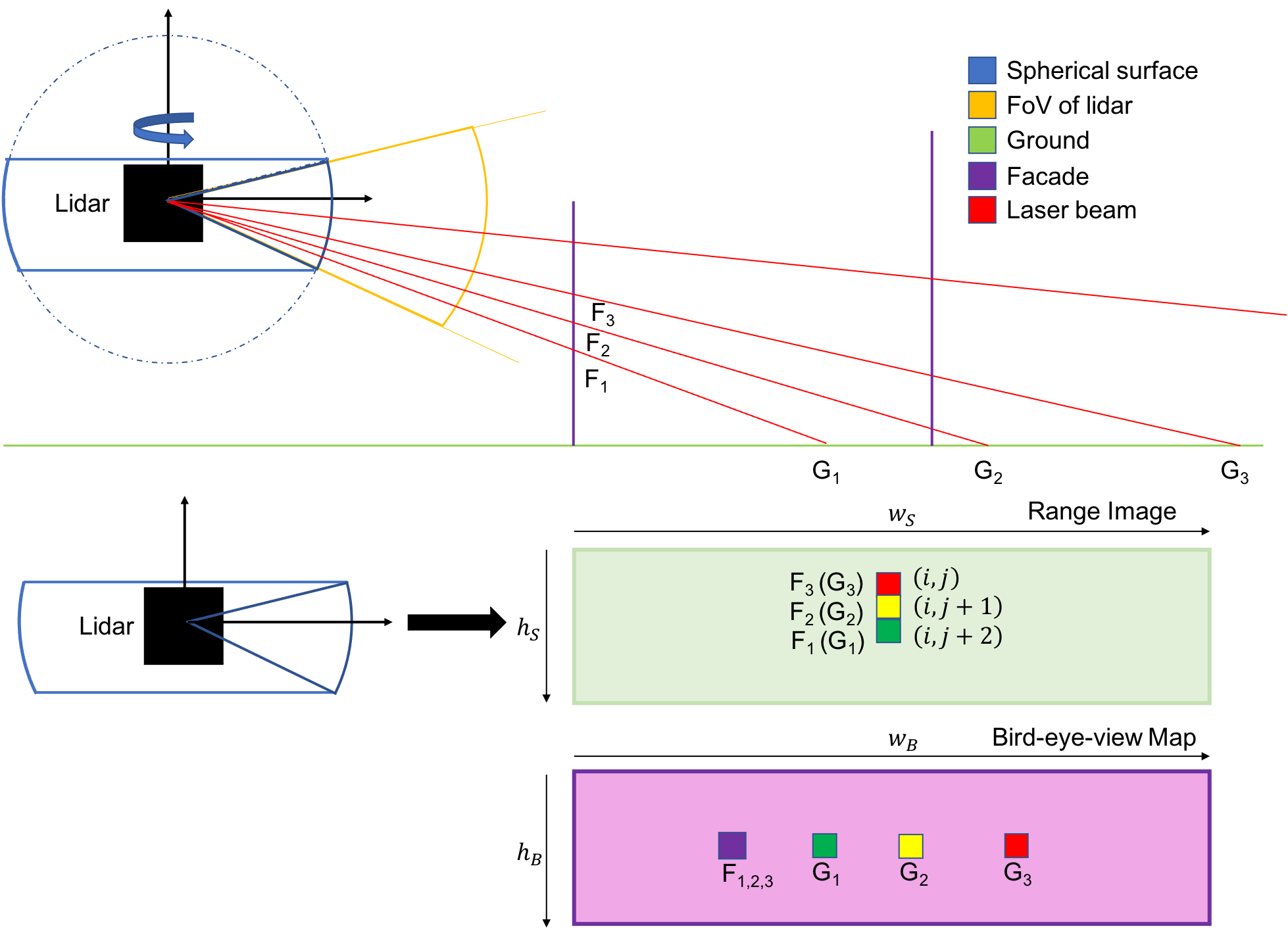
The distribution of perceived ground points is more sparser than non-ground ones. This incurs the issue that the adjacent pixels of ground points in spherical range image do not belong to the same local surface. We show an example in Fig. 3. Given three adjacent laser beams, the intersections of facade and ground are $F_{1},F_{2},F_{3}$ and $G_{1},G_{2},G_{3}$, respectively. Their corresponding pixels in the spherical range image are in the same column. Points lying on the facade perpendicular to laser beams are the exact nearest neighbors on one surface. However, the distance between adjacent pixels can be very large when the reflection surface is parallel to laser beams. Moreover, spherical range image divides the space by angle, which means that plenty of ground points between $\overline{G_{1}G_{2}}$ or $\overline{G_{2}G_{3}}$ would project into same pixel especially long range ground points. This will lead to the incorrect correspondence assignments and large errors in estimating the normal of ground region by the conventional spherical range image.

To deal with the above problem, we suggest to make use of bird’s-eye-view (BEV) map in order to taken into careful consideration of the abundant ground information, which greatly reserves the neighborhood relationship among ground points. As illustrated in Fig 2, BEV map is a top-down projection capturing LiDAR points information. Let $z$-axis denote the altitude direction. Since the space is divided on $x-y$ plane, the neighborhood information of ground surface is kept in BEV map. Unfortunately, the surface perpendicular to laser beams like those facade points $F_{1},F_{2},F_{3}$ are condensed into one pixel in BEV map. To this end, we propose a fusion approach by taking advantage of both non-ground spherical range image and ground BEV map in this paper.

Assuming that the current scan is observed in LiDAR coordinate system $L_{t}$ and the model is represented in the coordinate system $L_{t-1}$, where the subscript $t$ is the timestamp. We aim at finding the transformation $T^{L_{t-1}}_{L_{t}}$ that efficiently aligns the current scan with previous model. To avoid gimbal lock affected by Euler angle representations, we parameterize the transformation by $T^{L_{t-1}}_{L_{t}}\in\mathrm{SE(3)}$, which is denoted as $T^{t-1}_{t}$ for simplicity. Specifically, we employ an adaptive weighting strategy to fuse the non-ground cost $E_{S}$ and ground cost $E_{G}$, which forms the following minimization problem:

where $w=w_{1}w_{2}$ is the product of two coefficients. $w_{1}=0.7$ is a user-defined weight to balance the number of non-ground and ground points, and $w_{2}$ is the inlier ratio between the non-ground points and ground ones.

Obviously, the above problem is a nonlinear least squares minimization that can be efficiently solved through an iterative Gauss-Newton algorithm. Considering the large pose changes, we employ a constant acceleration scheme to initialize the transformation ${T^{t-1}_{t}}$. At each iteration, the pose update $\Delta T\in{\mathfrak{se}(3)}$ is estimated by $\Delta T=\left(J^{T}J\right)^{-1}J^{T}\mathbf{e}$, where $\mathbf{e}$ denotes the residual vector. $J\in\mathbb{R}^{1\times 6}$ is weighted Jacobian matrix as below:

where $J_{S}$ is the Jacobian of non-ground term, and $J_{G}$ is the Jacobian of ground term. The relative pose estimation $T^{t-1}_{t}$ is iteratively updated by $T^{t-1}_{t}=\exp(\Delta T)T^{t-1}_{t}$ until the convergence, where $\exp(\cdot):\mathfrak{se}(3)\mapsto SE(3)$ is the exponential map in Lie Algebra.

The input data acquired from LiDAR is usually unordered 3D point clouds, which can be mapped into an organized 2D range image by spherical projection as in [21, 11]. Therefore, the projection data association can be employed to very efficiently perform millions of nearest neighborhood search tasks in parallel. Given a scanned point $p=(x,y,z)^{T}$, the mapping function from the Cartesian to its corresponding spherical coordinate is defined as follows:

where $r$ denotes the range. $\theta$ is the azimuth, and $\phi$ represents the elevation component. They are constrained by $r\geq 0$, $-\pi<\theta\leqslant\pi$, and $-\pi/2<\phi\leqslant\pi/2$.

In this paper, the spherical range image is treated as a 2D search table $s(\theta,\phi)$, which stores the index of the Cartesian coordinates at azimuth $\theta$ and elevation $\phi$. The final image coordinates $(u,v)$ is converted by the spherical projection function $\Pi_{S}:\mathbb{R}^{3}\mapsto\mathbb{R}^{2}$,

where $f=f_{up}+f_{down}$ is the vertical field-of-view of the LiDAR sensor. $w_{S}=2048$ and $h_{S}=80$ are the width and height of spherical range image, respectively.

We deal with non-ground points using spherical range image by taking advantage of efficient projective data association. As in [10], the spherical range image is denoted as the vertex map $\mathcal{V}_{D}:\mathbb{R}^{2}\mapsto\mathbb{R}^{3}$, and its corresponding normal map is $\mathcal{N}_{D}$. Drifting usually occurs in the frame-to-frame registration due to error accumulation. To alleviate this issue, we adopt a frame-to-model method, where the model is represented by the vertex map $\mathcal{V}_{M}$ and normal map $\mathcal{N}_{M}$. Thus, we minimize the point-to-plane error to estimate the relative pose change as below:

where each vertex $\mathbf{u}\in\mathcal{V}_{D}$ is projectively associated to the model vertex $\mathbf{v}_{u}\in\mathcal{V}_{M}$ and its normal $\mathbf{n}_{u}\in\mathcal{N}_{M}$ via

Thus, the non-ground Jacobian $J_{S}$ can be computed as follows:

where $[\mathbf{v}_{u}]_{\times}$ denotes the skew symmetric matrix of vector $\mathbf{v}_{u}$.

As shown in Eqn. 8, the accuracy of Jacobian is heavily dependent on normal estimation, which is also essential to building the correspondences and computing the residual. Therefore, surface normal is the key to precisely predict the pose update. The conventional methods [11, 10] simply compute the normal through the cross product of local image gradients that may not belong to the same local planar region. This incurs the large errors in normal estimation. To this end, we propose a novel robust range adaptive normal estimation with two outlier rejection criteria.

In general, a plane is defined by the equation $n_{x}x+n_{y}y+n_{z}z-d=0$, where $(x,y,z)^{T}$ lies on the plane and $(n_{x},n_{y},n_{z},d)$ are the corresponding plane parameters. Given a subset of 3D points $\mathbf{p}_{i}$, $i=1,2,\cdots,k$ of the local surface, finding the optimal normal vector $\mathbf{n}=(n_{x},n_{y},n_{z})$ is a least square minimization on error $e$ as below:

which has a closed-form solution by eigen-decomposition. The covariance matrix $\Sigma$ explains the geometric information of the given local surface, which is defined as follows:

where $\bar{p}$ is the centroid of the point cloud subset. Using Eigen decomposition, $\Sigma\in R^{3\times 3}$ can be decomposed into three eigenvectors $\mathbf{v}_{1}$, $\mathbf{v}_{2}$ and $\mathbf{v}_{3}$, whose eigenvalues are in descending order $\lambda_{1}\geq\lambda_{2}\geq\lambda_{3}$. The least eigenvalue $\lambda_{3}$ indicates the variations along the surface normal $\mathbf{n}$ that is equal to its eigenvector $\mathbf{v}_{3}$. Moreover, we employ the surface curvature $\sigma_{\mathbf{p}_{i}}$ at $\mathbf{p}_{i}$ to select the salience planar feature:

With the spherical range image, we can visit a nearest neighbor with the time complexity of $O(1)$ for a small patch having the size of $(l_{x},l_{y})$, whose center location $\mathbf{p}$ is determined by its $(u,v)$ coordinates in range image. In the outdoor environment, the radius of LiDAR points have large variations within a scan, where the search window with the fixed size may not be effective. To account for the radius changes, we introduce a range adaptive searching window to select the nearest neighbors, in which the patch size is set according to the radius $r$, searching range threshold $\delta=0.3$m and range image resolution $(w_{S},h_{S})$:

where $l_{x}^{\max}=13$, $l_{y}^{\max}=7$, $l_{x}^{\min}=5$, and $l_{y}^{\min}=3$ denote the maximum and minimum searching range, respectively.

Due to the discontinuities at boundaries and multiple reflectance, the decomposition of covariance matrix is very sensitive to outliers. To reject the large outliers, we suggest two effective criteria. A point $\mathbf{p}$ is considered as an outlier if half points have the distance to the reference larger than the threshold $\sigma_{r}=0.5$m.

Another criterion is based on the point-to-plane distance $d_{p2p}=(q-p)^{T}\cdot\mathbf{n}_{p}$. A point is marked as outlier when its point-to-plane distance $d_{p2p}$ is large than the threshold $\sigma_{z}=0.5$, $d_{p2p}>\sigma_{z}$.

To efficiently obtain the ground segmentation, we employ a fast thresholding algorithm using the spherical range image. Since the height of LiDAR center with respect to road surface $h_{g}$ can be estimated from calibration, the ground point candidates need satisfy the condition $h_{p}-h_{g}>\delta_{h_{1}}$ and $h_{g}-h_{p}>\delta_{h_{2}}$. $h_{p}$ represents the height of candidate point. $\delta_{h_{1}}=0.5$m and $\delta_{h_{2}}=1$m are two thresholding values in height direction.

Pixels in the column $v$ of spherical range image are regarded as lying in the same azimuth space. If two adjacent pixels are in ground, the angle change in height direction should be less than a small threshold $\delta_{\theta}=5^{\circ}$. A valid pixel at $(u,v)$ in range image indexes a 3D point $\mathbf{p}$ in Cartesian coordinate. We find the first valid points up $\mathbf{p}_{up}$ and down $\mathbf{p}_{down}$ whose coordinates in range image are $(u,v+i)$ and $(u,v-j)$, $i,j=1,2,3,\dots$. The angle change in two directions can be computed as below:

where $\left\lfloor\cdot\right\rfloor_{(\cdot)}$ denotes the normal length in the specific direction. The ground points are selected by the angle changes below the threshold $\theta_{up}<\delta_{\theta}$ and $\theta_{down}<\delta_{\theta}$. The remaining points are regarded as non-ground.

Similar to the spherical range image, bird’s-eye-view projection also maps 3D Cartesian coordinate points into a 2D map. Specifically, each ground point $\mathbf{p}=(x,y,z)^{T}$ is converted into its corresponding coordinates $(u,v)$ in BEV map by the projection function $\Pi_{G}:\mathbb{R}^{3}\mapsto\mathbb{R}^{2}$ defined as follows:

where $w_{B}=120$m and $h_{B}=60$m are the predefined scope in the two direction of BEV image. $s_{x}=0.1$m and $s_{y}=0.1$m represent the resolution of the BEV map in two directions.

In this paper, we suggest to make use of the 2D BEV map to effectively align the ground points of the current scan with the previous model map $\mathcal{B}_{M}$ through the projection data association. BEV vertex map $\mathcal{B}_{G}:\mathbb{R}^{2}\mapsto\mathbb{R}^{3}$ can be treated as a 2D search table for the fast nearest neighbor search, where each pixel contains the 3D ground points. Let $\mathbf{n}_{g}$ denote the surface normal for ground point, the cost function $E_{G}$ can be derived as below

where each vertex $\mathbf{g}\in\mathcal{B}_{G}$ is projectively associated to a model vertex $\mathbf{v}_{g}\in\mathcal{B}_{M}$ via

The Jacobian $J_{G}$ for the ground cost $E_{G}$ can be computed by

where $[\mathbf{v}_{g}]_{\times}$ denotes the skew symmetric matrix of vector $\mathbf{v}_{g}$.

In contrast to the non-ground cost $E_{S}$, the surface normal $\mathbf{n}_{g}$ for ground point is not precomputed during the feature extraction stage. As the neighbors of ground points in a scan are usually far away from each other, the surface curvature of range image may not reflect the true geometry structure. Therefore, the normals of ground points are computed online while minimizing the ground cost $E_{G}(\mathcal{B}_{G},\mathcal{B}_{M})$. After projecting the current ground point $\mathbf{g}$ onto the previous local map $\mathbf{v}_{g}$, we retrieve the five closest points of $\mathbf{v}_{g}$ to calculate the surface normal in the BEV model map. By making use of the 2D BEV image, it is very efficient to find the candidate points in a predefined local patch on GPU.

References

- [1] C. Cadena, L. Carlone, H. Carrillo, Y. Latif, D. Scaramuzza, J. Neira, I. Reid, and J. J. Leonard, “Past, present, and future of simultaneous localization and mapping: Toward the robust-perception age,” IEEE Transactions on robotics, vol. 32, no. 6, pp. 1309–1332, 2016.
- [2] R. Mur-Artal, J. M. M. Montiel, and J. D. Tardos, “Orb-slam: a versatile and accurate monocular slam system,” IEEE transactions on robotics, vol. 31, no. 5, pp. 1147–1163, 2015.
- [3] J. Zhu, “Image gradient-based joint direct visual odometry for stereo camera.” in IJCAI, 2017, pp. 4558–4564.
- [4] P. J. Besl and N. D. McKay, “Method for registration of 3-d shapes,” in Sensor fusion IV: control paradigms and data structures, vol. 1611. International Society for Optics and Photonics, 1992, pp. 586–606.
- [5] M. Muja and D. G. Lowe, “Fast approximate nearest neighbors with automatic algorithm configuration.” VISAPP (1), vol. 2, no. 331-340, p. 2, 2009.
- [6] A. Geiger, P. Lenz, and R. Urtasun, “Are we ready for autonomous driving? the kitti vision benchmark suite,” in 2012 IEEE Conference on Computer Vision and Pattern Recognition. IEEE, 2012, pp. 3354–3361.
- [7] J. Zhang and S. Singh, “Loam: Lidar odometry and mapping in real-time.” in Robotics: Science and Systems, vol. 2, no. 9, 2014.
- [8] P. Biber and W. Straßer, “The normal distributions transform: A new approach to laser scan matching,” in Proceedings 2003 IEEE/RSJ International Conference on Intelligent Robots and Systems (IROS 2003)(Cat. No. 03CH37453), vol. 3. IEEE, 2003, pp. 2743–2748.
- [9] A. Hornung, K. M. Wurm, M. Bennewitz, C. Stachniss, and W. Burgard, “Octomap: An efficient probabilistic 3d mapping framework based on octrees,” Autonomous robots, vol. 34, no. 3, pp. 189–206, 2013.
- [10] J. Behley and C. Stachniss, “Efficient surfel-based slam using 3d laser range data in urban environments.” in Robotics: Science and Systems, vol. 2018, 2018.
- [11] T. Whelan, S. Leutenegger, R. Salas-Moreno, B. Glocker, and A. Davison, “Elasticfusion: Dense slam without a pose graph.” Robotics: Science and Systems, 2015.
- [12] J.-E. Deschaud, “Imls-slam: scan-to-model matching based on 3d data,” in 2018 IEEE International Conference on Robotics and Automation (ICRA). IEEE, 2018, pp. 2480–2485.
- [13] M. Brossard, S. Bonnabel, and A. Barrau, “A new approach to 3d icp covariance estimation,” IEEE Robotics and Automation Letters, vol. 5, no. 2, pp. 744–751, 2020.
- [14] N. Chebrolu, T. Läbe, O. Vysotska, J. Behley, and C. Stachniss, “Adaptive robust kernels for non-linear least squares problems,” IEEE Robotics and Automation Letters, vol. 6, no. 2, pp. 2240–2247, 2021.
- [15] A. Censi, “An icp variant using a point-to-line metric,” in 2008 IEEE International Conference on Robotics and Automation. IEEE, 2008, pp. 19–25.
- [16] K.-L. Low, “Linear least-squares optimization for point-to-plane icp surface registration,” Chapel Hill, University of North Carolina, vol. 4, no. 10, pp. 1–3, 2004.
- [17] J. Demantké, C. Mallet, N. David, and B. Vallet, “Dimensionality based scale selection in 3d lidar point clouds,” in Laserscanning, 2011.
- [18] C. Ulaş and H. Temeltaş, “3d multi-layered normal distribution transform for fast and long range scan matching,” Journal of Intelligent & Robotic Systems, vol. 71, no. 1, pp. 85–108, 2013.
- [19] A. Segal, D. Haehnel, and S. Thrun, “Generalized-icp.” in Robotics: science and systems, vol. 2, no. 4. Seattle, WA, 2009, p. 435.
- [20] T. Shan and B. Englot, “Lego-loam: Lightweight and ground-optimized lidar odometry and mapping on variable terrain,” in 2018 IEEE/RSJ International Conference on Intelligent Robots and Systems (IROS). IEEE, 2018, pp. 4758–4765.
- [21] S. Izadi, D. Kim, O. Hilliges, D. Molyneaux, R. Newcombe, P. Kohli, J. Shotton, S. Hodges, D. Freeman, A. Davison et al., “Kinectfusion: real-time 3d reconstruction and interaction using a moving depth camera,” in Proceedings of the 24th annual ACM symposium on User interface software and technology, 2011, pp. 559–568.
- [22] X. Chen, A. Milioto, E. Palazzolo, P. Giguere, J. Behley, and C. Stachniss, “Suma++: Efficient lidar-based semantic slam,” in 2019 IEEE/RSJ International Conference on Intelligent Robots and Systems (IROS). IEEE, 2019, pp. 4530–4537.