Efficient Exact Enumeration of Single-Source Geodesics on a Non-Convex Polyhedron
Abstract.
In this paper, we consider enumeration of geodesics on a polyhedron, where a geodesic means locally-shortest path between two points. Particularly, we consider the following preprocessing problem: given a point on a polyhedral surface and a positive real number , to build a data structure that enables, for any point on the surface, to enumerate all geodesics from to whose length is less than . First, we present a naive algorithm by removing the trimming process from the MMP algorithm (1987). Next, we present an improved algorithm which is practically more efficient on a non-convex polyhedron, in terms of preprocessing time and memory consumption. Moreover, we introduce a single-pair geodesic graph to succinctly encode a result of geodesic query. Lastly, we compare these naive and improved algorithms by some computer experiments.
Key words and phrases:
Geodesics; enumeration; locally-shortest paths; polyhedral geodesics; discrete geodesics1. Introduction
The shortest path problem is a fundamental problem in the field of discrete algorithm, which is also practically important and has been extensively investigated. Particularly, there is a variety of work for the single-source shortest path problem on a polyhedral surface [1, 2, 3, 4]. The single-source shortest path problem on a polyhedron is defined as follows: An input to the problem consists of a polyhedron and a point on . The task is to find a shortest path from to for all vertices of . Mitchell, Mount and Papadimitriou [1] first presented an efficient algorithm for the problem, which computes the shortest path between two points on a polyhedron. Following [1], there has been a variety of work for the single-source shortest path problem on a polyhedron, including the CH algorithm by Chen and Han [2] and the ICH algorithm by Xin and Wang [3]. Moreover, a graph-based approach to the vertex-to-vertex all-pairs shortest path problem on a polyhedron is given based on the Saddle Vertex Graph by Ying, Wang, and He [4]. On the other hand, geodesics on a smooth surface are defined to be locally shortest paths in differential geometry, and have applications in subfields of physics such as mechanics and optics, but relatively less attention has been attracted in the discrete algorithm field. Particularly, the problem of enumerating locally shortest geodesics with given two endpoints on a polyhedron has not been studied to date.
In this paper, firstly we define geodesics on a polyhedron, and formulate the single-source geodesics enumeration problem as a generalization of the single-source shortest path problem on a polyhedron. The problem is stated as follows: given a point on a polyhedral surface and a positive real number , an algorithm is asked to build a data structure for queries of enumeration of all (possibly non-shortest) geodesics shorter than , which goes from to arbitrarily chosen point on the surface. Such a query is called a geodesics enumeration query. For the purpose, we first introduce a naive version of the data structure, called the complete geodesic interval tree, that is computed from a point on a polyhedral surface and a positive real number in time using space, where is the number of intervals contained in . Next, we consider the problem of reducing the number of intervals in , which leads to the reduction of time and space of enumerating geodesic paths. To tackle this problem, we present an improved version of the data structure, called the reduced geodesic interval tree, where we remove the overlaps between adjacent intervals around a hyperbolic vertex. Moreover, we show that the reduced geodesic interval tree allows a query result to be succinctly encoded as a single-pair geodesic graph. By our experiments, it was shown that the reduced geodesic interval tree is smaller than the complete geodesic interval tree, and the reduced geodesic interval tree is better in practical running time and memory consumption.
2. Preliminaries
Throughout this paper, we simply use the term polyhedron (plural polyhedra) to mean a (possibly non-convex) polyhedral surface, not solid polyhedron. We deal with simplicial (which means triangulated) orientable polyhedra in , and the symbol is dedicated to mean such one.
Definition 2.1.
Let be a vertex of . Let be the sum of angles around (measured along the faces) and we call it the total angle of . Following [5], we say that
-
•
if , is spherical;
-
•
if , is Euclidean;
-
•
if , is hyperbolic.


Remark 2.2.
If is convex, every vertex is spherical or Euclidean. Note that the angle defect can be interpreted as the discrete Gaussian curvature at . For example, a discrete analog of the Gauss-Bonnet theorem holds for a polyhedron [6].
We define a geodesic as follows:
Definition 2.3.
(geodesics) Let be a path connecting and on . We say that is a geodesic if and only if:
-
(1)
is straight inside any face, and where passes through an edge sequence , is straight on the unfolding obtained from ;
-
(2)
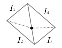
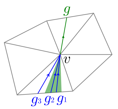
where passes through a vertex, the angle at the vertex made on the both sides of are greater than or equal to (see Figure 2).
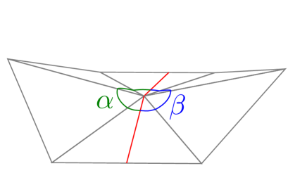
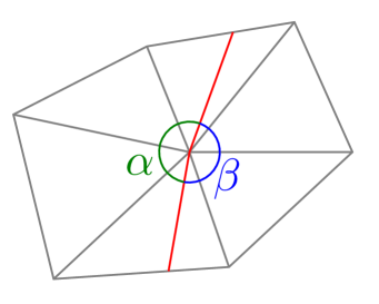
Left: 3D perspective view, right: top view
Lemma 2.4.
A geodesic never passes through any spherical vertex.
Proof.
Since the angle and at the vertex made on the both sides of satisfy and (see Figure 2), the total angle of this vertex is . ∎
Remark 2.5.
Although a geodesic does not pass through a spherical vertex, its endpoints may be spherical vertices. Moreover, a geodesic may pass through an arbitrarily close neighbor of a spherical vertex.
Remark 2.6.
Intuitively, a geodesic is a locally-shortest path. Geodesics on a polyhedron, defined above, can be used to approximate geodesics on a smooth surface, defined in differential geometry. Nevertheless, there are some important differences between the discrete geodesics and the smooth geodesics. Let us take a look at some examples.
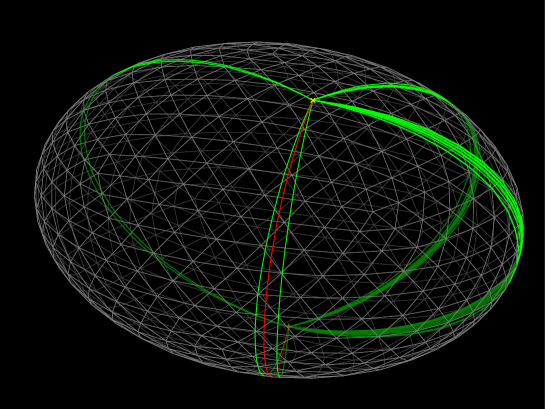
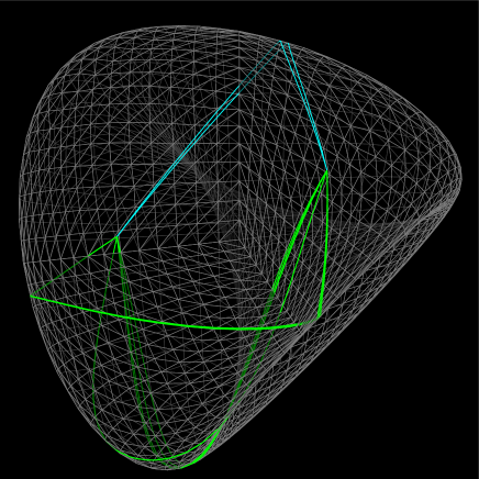
Figure 3 shows the shortest geodesic (red) and other geodesics (green) on a discrete ellipsoid. Since it is convex (and does not have Euclidean vertices), every vertex is spherical and geodesics pass through no vertices. Instead, there are often multiple similar geodesics that differ in how they “bypass” the vertices. As a result, when a smooth surface is discretized into a polyhedron, a single geodesic on the smooth surface often corresponds to multiple geodesics on the discretized polyhedral surface.
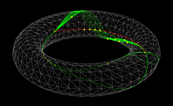
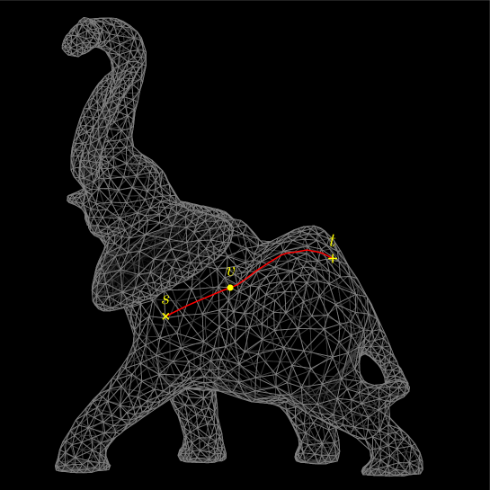
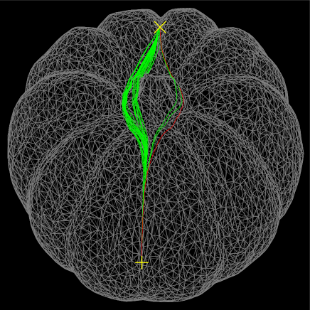
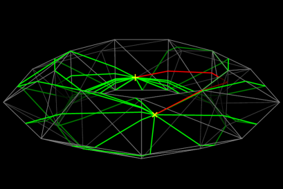
If the polyhedron has hyperbolic vertices, the geodesics can pass through them. Figure 4 shows that the shortest geodesic (red) passes through consecutive four hyperbolic vertices, as well as some of non-shortest geodesics (green) also pass through several vertices. These vertices are marked in yellow. In general, a geodesic can be decomposed into a sequence of geodesics passing through no hyperbolic vertices. We call them primitive geodesics.
Definition 2.7 (primitive geodesic).
A geodesic passing through no hyperbolic vertices is called a primitive geodesic.
Remark 2.8.
Endpoints of a primitive geodesic may be hyperbolic vertices.
2.1. Our problem
Let be a simplicial polyhedron in . When we give a source on , we want to compute all geodesics from to an arbitrary point on . Since we have infinitely many choice of , we consider a query that inputs and outputs these geodesics. And yet, there are likely to be infinitely many such geodesics and we give an upperbound of their length to obtain finite result.
It is widely known that single-source shortest path problems (SSSPs) for graphs or polyhedra can be efficiently solved using a queue or a priority queue. Here, we can think of a generalization of SSSPs, namely, single-source geodesics enumeration problem on a polyhedron.
Definition 2.9 (single-source geodesics enumeration problem).
Suppose that is a simplicial polyhedron in , is a point on and is a positive real number. We define our single-source geodesics enumeration problem to be the problem of building data structure that enables to query, for any point on , all geodesics from to whose length is less than . We call an algorithm for this problem a single-source geodesics enumeration algorithm, or simply geodesics enumeration algorithm.
3. Related work
As far as we know, there is no prior work for enumerating geodesics on a polyhedron. However, there is a variety of research relating to geodesics on polyhedral meshes.
3.1. Shortest geodesics
The shortest path problem on a polyhedron has been extensively researched. On a polyhedron without boundary, a shortest path is a geodesic in our sense [1], thus the shortest path problem is equivalent to the shortest geodesic problem. Shortest geodesic algorithms can be divided into exact algorithms and approximate algorithms. Since the interest of this paper is exact algorithms, approximate algorithms are not discussed in detail here. Detailed survey of this topic is given by [7, 8].
3.1.1. Interval propagation algorithms for the SSSP
The MMP algorithm given by Mitchell, Mount and Papadimitriou [1] is an important exact algorithm for the SSSP on a polyhedron. It retains intervals on each edge, so that the shortest path to any point within an interval has the same combinatorial structure (faces, edges and vertices). Information required to reconstruct geodesics is appended to these intervals. However, each interval only represents geodesics passing through a particular face among the two faces incident to the edge. This can be interpreted that each interval is assigned to a directed edge and only represents geodesics through one side (in the original paper, it is the right side along the directed edge).
In the earliest stage of the MMP algorithm, intervals are created only for the edges facing . Each interval is propagated using the continuous Dijkstra scheme. When it detects a shortest geodesic reaching a hyperbolic vertex, it generates the intervals representing the geodesics passing through that vertex. Intervals on the same directed edge are ordered, and a newly-propagated interval is inserted into the ordered list of the intervals already-existing on the directed edge. Then, it performs trimming among the new interval and adjacent intervals. By trimming, intervals are cut to ensure shortestness against other intervals, and intervals on a directed edge become disjoint. Intervals may become empty as a result of trimming, and such intervals are not propagated. When no non-empty intervals are newly created and the priority queue becomes empty, the algorithm terminates and outputs the shortest geodesics. Its computational complexity given by the original authors is time and space, where is the number of the edges of the input polyhedron. However, according to an experiment by Surazhsky et al. [9], its practical complexity is subquadratic and could be considered as approximately time and space. They analyzed the reason behind it as that, the number of intervals per edge is approximately in practice, despite the estimation by MMP.
Most of exact algorithms for the SSSP on a polyhedron, published after the MMP algorithm, contain the concept of interval propagation. The CH algorithm by Chen and Han [2] uses a FIFO queue instead of a priority queue. Its theoretical complexity is time and space, but its practical performance is not as good as the MMP algorithm. The ICH (improved CH) algorithm by Xin and Wang [3] introduces into the CH algorithm a priority queue as well as several new rules to exclude intervals not contributing to any shortest paths. In theory, the usage of a priority queue increases its time complexity to , but greatly improves its practical performance. While the MMP algorithm requires inserting an interval into an ordered list and solving a quadratic equation to get the intersection of the interval and certain hyperbola, the ICH algorithm does not. As a result, the ICH algorithm may outperform the MMP algorithm despite the ICH algorithm may generate more intervals than the MMP algorithm. Moreover, the ICH algorithm does not require the history of the propagated intervals to be retained. As a result, the space complexity of the ICH algorithm is , which is significantly smaller than the MMP algorithm.
3.1.2. Saddle Vertex Graph
The Saddle Vertex Graph (SVG) by Ying, Wang and He [4] is an approach to the vertex-to-vertex all-pairs shortest path problem on a polyhedron. They noticed that a shortest geodesic between two hyperbolic vertices may be shared by multiple longer shortest geodesics, and reduced the problem to the well-known shortest path problem on a graph by precomputing shortest primitive geodesics connecting two vertices. However, when the given polyhedron is convex, it has no hyperbolic vertices and there is no difference from precomputing the shortest path for every pair of vertices. However, they observed real-world meshes contain 40-60% hyperbolic vertices and more than 90% of shortest paths pass through at least one hyperbolic vertex. Also, they considered the exact SVG is too large to be tractable for large meshes and proposed a method to sparsify it, and evaluated error by computer experiments.
3.2. General geodesics
Geodesics, which are not limited to shortest, also have been researched in the context of geodesic tracing and path shortening.
3.2.1. Geodesic tracing
A classical problem about a smooth surface in differential geometry is to trace the smooth geodesic from a given point and a tangent direction . Concerning the corresponding problem on a polyhedron, this can be done at almost every point. However, a geodesic cannot proceed beyond a spherical vertex, and it cannot uniquely determine its direction when it hits a hyperbolic vertex. To cope with this problem, Polthier and Schmies suggested a straightest geodesic which goes through a vertex to halve the total angle of the vertex [5]. However, it is not necessarily locally-shortest anymore, and does not have continuity respect to and , i.e. it jumps when it moves onto or across a non-Euclidean vertex, thus its nature vastly differs from a geodesic on a smooth surface. To fill this gap, Cheng, Miao, Liu, Tu and He suggested a method to trace smooth geodesics on a tangent-continuous curved surface constructed from the input polyhedron using PN-triangles, and evaluated its accuracy by computer experiments [10].
3.2.2. Path shortening
In this approach, an input polyline on a polyhedron is shortened until it becomes a geodesic. The shortening process is performed according to local configuration of the path. It is implemented in e.g. [11, 12, 13] and they used it to refine a path obtained by Dijkstra’s algorithm on the edge graph or other approximate shortest path algorithms on the polyhedron.
Recently, a flip-based algorithm was developed by Sharp and Crane [14]. An initial path is given as an edge sequence, and until the path becomes a geodesic, the algorithm modifies the triangulation by flipping an edge so that the new shortened path is still on the edges of the new triangulation. It works on intrinsic triangulations of a polyhedron — that is, the new triangulation is intrinsically embedded in the original surface, and its edges are no longer straight when it is viewed as an object in . It allows the geometry of the original surface to remain unchanged by flipping. Their method can yield not only open geodesics but also closed geodesics. Although they did not give worst-case bounds, they proved that it always obtains a geodesic by finite operations, and observed that its practical running time is on the order of milliseconds.
4. Geodesics and intervals
To explain how intervals can be used to express geodesics, we begin with an observation of geodesics on a polyhedron. In Figure 5, a geodesic from the source , to on a face , is shown in red. Since passes through a vertex , it can be decomposed into the two primitive geodesics, between and between . By Definition 2.3 (1), a primitive geodesic can be unfolded into a line segment. Particularly, the primitive geodesic between can be unfolded into the line segment on the plane containing (Figure 6).
This unfolding of the geodesic between is shown in 2D in Figure 7. As a simple observation, when one moves in the region shaded in yellow, the line segment still gives a geodesic on the unfolding. This region is chosen so that the line segment does not go out of the unfolding and satisfies the condition (2) in Definition 2.3 at .
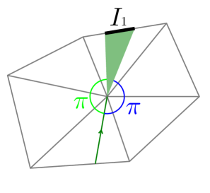
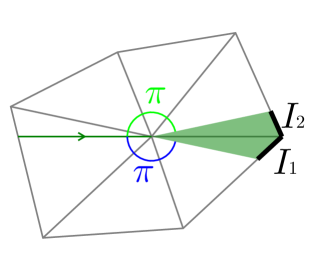
When is inside a face, one can extend the geodesic until hitting an edge, thus here we only consider geodesics to a point on an edge. We introduce concept of intervals generalizing the ones in the MMP algorithm (or other interval propagation algorithm) to express geodesics to a particular range on an edge. Figure 8 shows an outline of this expression. The yellow and green line segments represent the range of the intervals and indicate the range on which geodesics can be given in this unfolding. The region darkly shaded in their respective color indicates the region in which the interval is used in the geodesic query. As a remark, when a geodesic passes through no vertices, we consider the unfolding of the whole geodesic from , and when it passes through multiple vertices, we consider the unfolding of the primitive geodesic between the last vertex and .
Figure 9 shows the intervals to express the geodesics immediately after passing through a vertex. We call them pseudo-source intervals.
Definition 4.1.
An interval is defined to be the following data structure:
-
•
: the interval which generated (by propagation)
-
•
: the target edge
-
•
: the target face
-
•
: the target line segment on (identified with itself)
-
•
: the unfolded position of the last vertex
-
•
: the length of the geodesic between and the last vertex
It is used to express all geodesics reaching the line segment on the edge through the last vertex. If the geodesics have not passed through a hyperbolic vertex yet, is the unfolded position of and is 0.
We regard to be oriented so that is seen on the left side along . We define the starting point of with respect to this orientation. Moreover, has the following two functions:
-
•
:= the intersection point of and the line connecting and
-
•
:= (the distance of and ) +
The interval can yield a geodesic at if , and its length is given by .
Remark 4.2.
can be expressed in either the 3D global coordinate system or a 2D local coordinate system on . 2D local coordinates are slightly faster and memory efficient, as well as ensure that given coordinates are always on the plane. Our implementation uses the 3D global coordinate system in input and output, but uses a 2D local coordinate system in internal storage and computation, and converts one to the other when necessary. That means, our algorithms could run on a polyhedron in higher-dimensional Euclidean space as well.
Remark 4.3.
Our algorithms can also work on a self-intersecting polyhedral surface. In this case, geodesics are not bent at the intersection and pass through it as if there were no intersection — geodesics are completely defined locally. On the other hand, we assume the orientability of the surface, which may not be the case for a self-intersecting (or higher-dimensional) polyhedron. If this is an issue, one can take the orientable double covering of the surface, as demonstrated in Figure 10. In this figure, geodesics are computed on a discretized version of the orientable double covering, which is homeomorphic to the sphere, of the (non-orientable) Roman surface (a realization of the real projective plane in ). The source is given once, but the target is given twice, correspondingly to its two images on the double covering. In the figure, two different colors are used accordingly.
Remark 4.4.
Our implementation uses the half-edge data structure as the internal representation of a polyhedron, thus every edge is directed. Here the 2D local coordinate system is defined by the directed edge so that its origin is the starting point of , its positive direction is the direction of , its axis is orthogonal to the axis and any point inside has positive value. Complex numbers are convenient for expressing the local coordinates, because
-
•
we often need an 1D parametric coordinate on as well. Since a real number is considered to be a complex number whose imaginary part is zero, we can naturally treat it as a special case of 2D local coordinates;
-
•
when we express in the 2D local coordinate system, we need to apply coordinate transformation to propagate an interval. This transformation consists of 2D rotation and translation, which can be expressed in terms of complex multiplication and addition;
-
•
functions such as and are also useful to implement our algorithm.
5. Naive geodesics enumeration algorithm
We can make a naive geodesics enumeration algorithm by propagating intervals without the trimming process in the MMP algorithm. All intervals generated in this way form a tree structure by the Parent pointer. we call it the complete geodesic interval tree or the complete GIT.
This algorithm firstly performs initialization of generating several intervals, and proceeds by processing events. We define propagation to be the act of generating one or more new intervals by processing an event. Events consist of the following two types:
-
•
edge event : when a geodesic given by reaches for the first time
-
–
this event is associated with
-
–
time of occurrence: (the distance of and ) +
-
–
-
•
vertex event : when a geodesic reaches a vertex
-
–
this event is associated with the interval of which the starting point is
-
–
time of occurrence: (the distance of and ) +
-
–
We introduce an event queue to manage the order of events. It is a priority queue, and lets the algorithm process events in the ascending order of their time of occurrence.
The outline is described in Algorithm 1 as a pseudocode.
Remark 5.1.
In Algorithm 1 (and Definition 2.9), we assume that is given ahead of time. Alternatively, we can rewrite the line 4 with another arbitrary terminating condition (or as an infinite loop which can be stopped by a human), and when the loop terminates, can be obtained as the time of occurrence of the top event of . This also applies to the improved algorithm in the next section.
5.1. Initialization
Firstly, the intervals for all edges facing are generated. Figure 11 shows the cases of being inside a face (left), inside an edge (middle), and at a vertex (right). For each of these initial intervals, is Null, is , is 0, is the whole , and is the face containing both and . For each , the associated edge event and vertex event are inserted into the event queue. (Algorithm 2)
5.2. Procedure for edge events
When an edge event occurs, the associated interval is projected from into the opposite edges of (Figure 12). The projection result is on either one edge (left) or two edges (right). For each newly created interval (left: , right: ), , and is the triangular face in Figure 12. is obtained by certain 3D rotation around to make it coplanar with . For each , the associated edge event is inserted into the event queue. In the two-interval case (right), the vertex event at the intermediate vertex is associated with the interval starting at (that is ) and inserted into the event queue. (Algorithm 3)
5.3. Procedure for vertex events
When a vertex event occurs, the associated interval is recorded on as it gives the geodesic arriving at . If is hyperbolic, one or more pseudo-source intervals are generated. In Figure 9, one interval in the left subfigure, two intervals in the right are generated. For each newly-created interval , , , is the length of the geodesic to (= the time of occurrence of this event), and the associated edge event and vertex event (if exists) are inserted into the event queue. (Algorithm 4)
5.4. Geodesics enumeration query
After building the complete geodesic interval tree, it can accept the geodesics enumeration query which inputs a point on and outputs the set of geodesics from to , whose length is less than . First, we must determine which intervals are responsible for the output. It can be done using the GetIntervals function:
Definition 5.2.
We define the GetIntervals() function as follows:
-
•
If is a vertex , GetIntervals() returns the set of intervals recorded on .
-
•
If is on an edge , GetIntervals() returns the set of all generated intervals such that , and .
-
•
If is on a face , GetIntervals() returns the set of all generated intervals such that , and .
For each obtained interval, using Algorithm 5, the geodesic is constructed from to by backtracking . The whole procedure is given by Algorithm 6. In the pseudocode, Intersect is the function of getting the intersection, and AddFront is the operation of inserting a point at the front of the list.
6. Improved geodesics enumeration algorithm
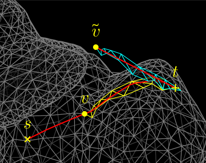
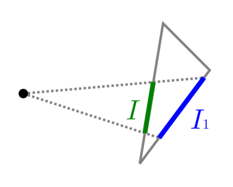
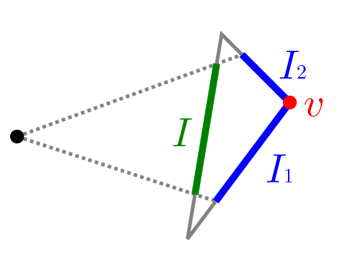
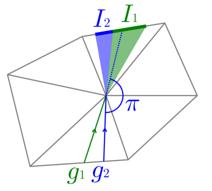
The difference between the MMP algorithm and the geodesics enumeration algorithm in the previous section based on the complete geodesic interval tree is that, since we are also interested in non-shortest geodesics, our intervals are never trimmed. However, this change largely increases the computational complexity. Here, when is non-convex, we can reduce required amount of time and memory by placing pseudo-source intervals without overlap. We can understand the redundancy of the naive algorithm using Figure 13. In the figure, the source is indicated as the yellow cross sign () and the target is indicated as the yellow plus sign (). While multiple geodesics are outgoing from , they merge at some hyperbolic vertices until reaching and they all share some part near . However, the naive algorithm cannot recognize and utilize this property; the shared part of the geodesics is independently encoded in multiple intervals and rediscovered for each geodesic during the query process. The basic idea of improvement is shown in Figure 14. In this figure, a geodesic already arrived at a hyperbolic vertex and yielded a pseudo-source interval . Now, another geodesic arrives at the vertex. Although can go through the dotted blue line, can be chosen to exclude the region already searched by . As we will see later, we can still restore all geodesics in the query process.
6.1. Procedure of reduction
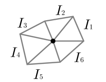
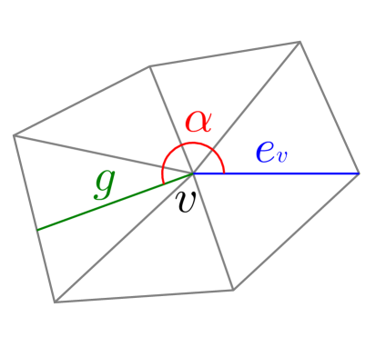
For the purpose of generalizing this argument, for each hyperbolic vertex , we arbitrarily choose an edge among those incident to and we fix the choice (Figure 15). It allows us to numericalize the direction of (seen from ) into (measured along the faces). When is incoming into , we call the incoming angle of , and when is outgoing from , we call the outgoing angle of . Also, we use the term outgoing angle range () to assert that all values within this range are considered as outgoing angles, here is the total angle of . By convention, if then is empty, and if then all values within are subject to the “mod ” operation.
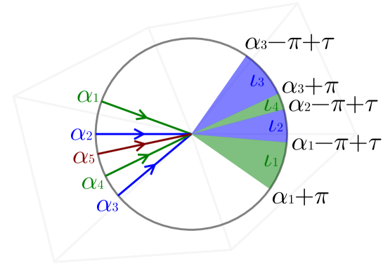
Let us explain how it works in the example shown in Figure 16. In this figure, the five geodesics of incoming angles (respectively) arrive at the vertex in this order. Here we assume . Each incoming angle is mapped to the corresponding outgoing angle range as follows:
-
(1)
: the outgoing angle range is and corresponding one pseudo-source interval (not shown) is generated.
-
(2)
: is limited by while is not, thus and two corresponding pseudo-source intervals (not shown) are created.
-
(3)
: neither nor limits , thus .
-
(4)
: is limited by and , thus .
-
(5)
: is limited by and thus is temporarily computed as . However, it is empty and no pseudo-source intervals are created.
Since the outline, initialization and procedure for edge events (Algorithm 1, 2, 3) are identical, we only explain the procedure for vertex events and geodesics query. All intervals generated in this way form a tree structure by the Parent pointer. we call it the reduced geodesic interval tree or the reduced GIT.
Remark 6.1.
In the reduced geodesic interval tree, only pseudo-source intervals generated at a common vertex are ensured to be disjoint. There may be an overlap between two non-pseudo-source intervals, or between a pseudo-source interval and a non-pseudo-source interval.
6.2. Procedure for vertex events
Like the naive version, when a vertex event occurs, the associated interval is recorded on . If is hyperbolic, it performs the procedure of the reduction explained in the previous subsection, and, if the resulting outgoing angle range is not empty, pseudo-source intervals are generated and the associated edge events and vertex events (if exist) are inserted into the event queue. (Algorithm 7)
6.3. Geodesics enumeration query
In this subsection, we discuss the geodesics enumeration query for the reduced geodesic interval tree, which inputs a point on and outputs the set of directed geodesics from to , whose length is less than .
In the complete geodesic interval tree, a geodesic is given for each pair by the ConstructGeodesic function (Algorithm 5). On the other hand, in the reduced geodesic interval tree, geodesics of the same path between the last vertex and are given together for the pair . The primitive geodesic between is given by the ConstructPrimitiveGeodesic function (Algorithm 8). The geodesic is constructed from to , and every time it hits a hyperbolic vertex, possible branches must be enumerated.
Let us take a look at the example illustrated in Figure 17. In this figure, each arrow indicates the direction from to , although the actual query is performed backwards. Let us assume that we have just found a geodesic outgoing from , and there are three geodesics , and incoming into , and each of and is connectable with as a geodesic while is not. Then, for each of and , we check it can satisfy the length upperbound, and if so, we connect it with and perform this process recursively.
In general, we can use a simple depth-first search here. For each interval , is the minimum of the depths of these geodesics grouped together. Since contains at least one geodesic represented by the pair if and only if the minimum of their lengths is less than , the procedure of the GetIntervals function (Definition 5.2) is identical. The whole procedure is given by Algorithm 9. In the pseudocode, RemoveLast is the operation of removing the last point from the sequence, and is used for endpoints of primitive geodesics not to appear twice.
6.4. Constructing single-pair geodesic graph
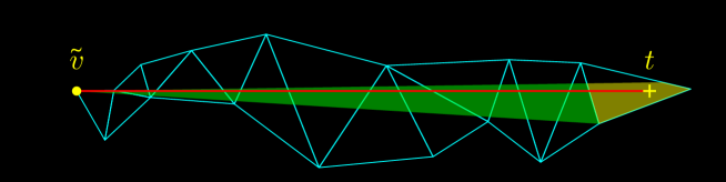
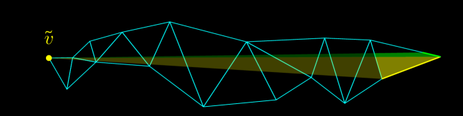
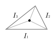
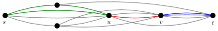
Since a geodesic is a sequence of primitive geodesics, we can reduce into a graph whose edges are primitive geodesics (Figure 18). We call it a single-pair geodesic graph, or simply a geodesic graph. It can be computed directly using the reduced geodesic interval tree.
Definition 6.2 (Single-pair geodesic graph).
The (single-pair) geodesic graph with respect to , is the directed graph satisfying the following conditions:
-
•
The vertices of are and the vertices of through which at least one geodesic in passes.
-
•
The edges of are the directed primitive geodesics connecting two vertices of , such that each of them is contained in at least one directed geodesic in .
Remark 6.3.
In a geodesic graph , and act as the source and the sink (respectively). Even if (resp. ) is placed at a vertex and geodesics pass through the vertex, we regard (resp. ), as a vertex of , to be distinct from any other vertex of . This convention allows us to design the algorithm without special treatment of (resp. ) being a vertex or not.
Remark 6.4.
A geodesic graph can have multi-edges. That is, there may exist pairs of edges such that the both endpoints coincide.
Remark 6.5.
Our geodesic graph bears some resemblance to the Saddle Vertex Graph (SVG) [4], but fundamentally differs as follows:
-
•
The SVG only considers shortest geodesics, while our geodesic graph considers non-shortest geodesics as well.
-
•
The SVG considers shortest geodesics for all pairs of vertices, while our geodesic graph only considers geodesics connecting and .
-
•
More importantly, the SVG is constructed before their geodesic query and the query is performed on the SVG, while our geodesic query is performed on the reduced geodesic interval tree and yields a geodesic graph. In other words, our geodesic graph is a representation of the query result.
Remark 6.6.
Our geodesic graph is an exact representation of the query result for the given , and . The naive representation often have many overlapped sub-geodesics. In this situation, we can compress them into a graph, eliminating redundancy that can be combinatorially reconstructed from the graph.
Remark 6.7.
A geodesic graph is constructed from to using Algorithm 10. We use a modified version of Dijkstra’s algorithm to determine the shortest possible length from for each primitive geodesic. We have two points to remark:
-
•
When is given, an interval can yield at most two primitive geodesics, and each primitive geodesic can be specified by the pair where is an interval and IsTarget is a Boolean value indicating whether the primitive geodesic ends with (otherwise it ends with the starting point of ). Note that IsTarget is set to be True only through the initialization of the algorithm since we regard to be a vertex of distinct from any other vertex (Remark 6.3). Since we can assume that no duplicated intervals are supplied by the GetIntervals function, we need to check visitedness only when IsTarget is set to False (the line 11–14).
-
•
In the line 23, is the length of the primitive geodesic given by . A conceptual figure is described in Figure 18. Let the red curve be the primitive geodesic and denoted as . Not necessarily all geodesics in contain . Let the green part and blue part be the subgraph of between and respectively through which a geodesic containing can pass (in general the green and blue subgraph may be overlapped). Then, the distance between on the green subgraph is , because of the construction method of the reduced geodesic interval tree. Moreover, the distance between on the blue subgraph is , because of the construction algorithm of the geodesic graph, which is derived from Dijkstra’s algorithm. Therefore the minimum length of geodesics between containing is , and is contained in as an edge if and only if it is less than .
7. Performance
In this section, since we evaluate both the naive version that generates a complete geodesic interval tree and the improved version that generates a reduced geodesic interval tree, we call them geodesic interval trees. Since the size of an output geodesic interval tree greatly depends on the geometry, it is difficult to express it only in terms of input size and . The efficiency of a reduced geodesic interval tree is due to its small size compared with the corresponding complete one, and we evaluate it by experiments in the next subsection. First, we state an output-sensitive complexity evaluation:
Theorem 7.1.
Let be a (complete or reduced) geodesic interval tree and be the number of intervals in it. The corresponding algorithm for generating runs in time and space.
Proof.
Since the number of the whole generated intervals is , the numbers of edge events and vertex events are . Thus, the size of the event queue is at any time. Therefore, the pop operation of the event queue takes time per event. Concerning processing time of an event, an edge event can be processed in constant time. A vertex event requires time proportional to the number of the intervals it generates, but it sums up to . Also, in the reduced version, the two adjacent incoming angles of an incoming angle must be acquired, but it can be done in time per event using a balanced binary search tree. Therefore, the time complexity is . On the other hand, since the required space is the whole output tree and the event queue, and each interval or event consumes constant space, the space complexity is . ∎
7.1. Experimental Result
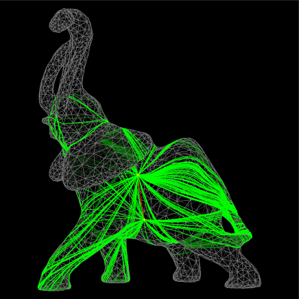
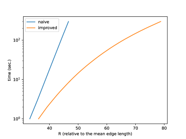
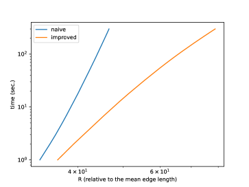
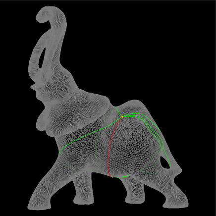
For the purpose of evaluating performance of our methods, we mainly use the Elephant mesh contained in the CGAL (Computational Geometry Algorithms Library) [15]. The proposed methods consist of two parts, i.e., the construction of a geodesic interval tree, and the geodesics query or the construction of a geodesic graph. Since the geodesics query consumes much less (often negligible) time, we only evaluate the performance of the construction of a geodesic interval tree, except Figure 34. We implemented our (single-threaded) algorithms in C++ and tested them using a machine with Intel(R) Core(TM) i9-9980XE CPU @ 3.00GHz and 128GB RAM running Linux. Except Figure 30, 30 and 34, we ran our program for 300 seconds and took statistics every second. In Figure 30 and 30, we manually recorded the amount of memory consumption measured by the OS, when it elapsed 10, 20, 30, 40, 60, 80, 100, 125, 150, 180, 210, 240, 270 and 300 seconds since each program started.
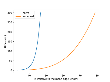
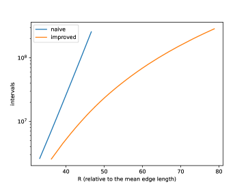
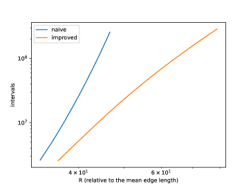
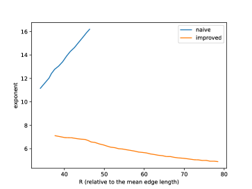
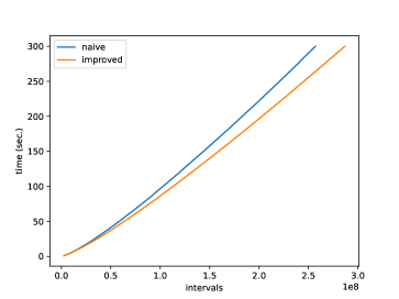
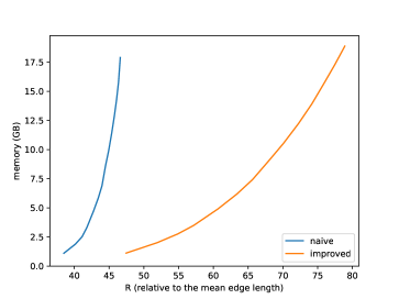
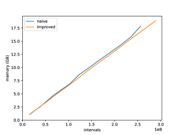
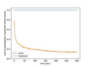
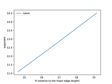
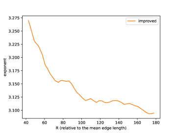
Relation of (normalized so that the mean edge length is 1) and running time is shown in Figure 25, and its log-linear plot and log-log plot are shown in Figure 25 and Figure 25. We can observe that the running time of the naive version grows exponentially to , while that of improved version grows more slowly. A log-linear plot and log-log plot of the total number of generated intervals are shown in Figure 25 and Figure 25, and they exhibit a pattern similar to that of the computation time. Figure 25 shows the slope of the log-log plot, i.e. , which can be considered as the exponent when is locally fit by ( and are constants). This value is increasing in the naive version but decreasing in the improved version, as increases. Figure 30 shows relation of and computation time, and exhibits a pattern similar to the quasilinear growth. Memory consumption is shown in Figure 30 (to ) and Figure 30 (to ). We can observe that the memory consumption seems to grow linearly to . Figure 30 shows the ratio of the number of propagating vertex events (vertex events that generated at least one interval) to the number of hyperbolic vertex events (vertex events that occurs at a hyperbolic vertex), among newly-processed events in one second. This value is 1 in the naive version but around 0.2 in the improved version in this instance, which means that, in the improved version, there are less vertex events that actually generate intervals compared with the naive version.
We also tested on a synthesized simple torus (Figure 31, 33, 33). We can observe that, for sufficiently large , the total number of generated intervals in the improved version is approximately . We have not established a theory, but we could guess the reason behind it as follows:
-
•
For sufficiently (very) large (and in generic cases), pseudo-source intervals are likely to “fill up” all angles around hyperbolic vertices so that no new pseudo-source intervals are generated.
-
•
In this situation, the area “swept” by the imaginary wavefront of intervals is . That is, the number of vertex events is likely to be . Since an interval in the wavefront splits into two intervals when it meets a vertex, the number of intervals in the wavefront is also likely to be . Since can be obtained by summing the size of each generation, it is likely to be .
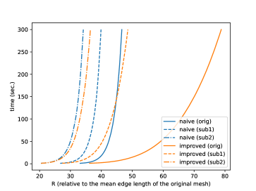
To evaluate relationship of smoothness of the mesh and performance, we used the recursively subdivided surfaces of Elephant using the Loop subdivision scheme [16]. In Figure 30, the computation time is shown for the original mesh (orig), and the surface subdivided once (sub1) and twice (sub2). Here is relative to the mean edge length of the original mesh. We can see that the computation time of the improved version becomes closer to that of the naive version as the mesh becomes more detailed. The reason behind it is that, pseudo-source intervals become more unlikely to overlap in the naive version, since the total angle of each vertex becomes closer to . The surface subdivided twice (sub2) from Elephant is used in Figure 34 to evaluate practical performance. The detail of the experiment is explained in the caption of this figure, but compared with the naive version, we can observe that the improved version took nearly half computation time and used approximately 56% memory to produce this result.
8. Conclusion
In this paper, we have formulated the single-source geodesics enumeration problem and presented two data structures for the problem: the complete geodesic interval tree and the reduced geodesic interval tree. Although we could not provide their worst-case bounds in terms of the input size, experiments suggested that the reduced geodesic interval tree is practically more efficient on a nonconvex polyhedron in terms of running time and memory consumption. On the assumption of reasonable complexity of the input mesh, our method allows geodesics to be computed in reasonable time, which opens up possibility of finding useful non-shortest geodesics which traditional shortest path algorithms cannot find.
We have given the complexity of our algorithms in terms of the size of the output geodesic interval trees. However, it largely depends on the geometry of the polyhedron, and a (non-trivial) complexity estimation is likely to include not only the input size (such as the number of vertices) and , but also geometrical characteristics of the polyhedron (such as discretized curvatures). Therefore, rigorous analysis of complexity may involve mathematical study of geodesics themselves on a polyhedron. Geodesics yielded by our method can be used to approximate geodesics on a smooth surface, although more accurate or efficient algorithms tailored for smooth surfaces could be developed.
Acknowledgements
The author sincerely appreciates Professor Hiroki Arimura and Professor Toru Ohmoto for giving many valuable advices.
References
- [1] J. S. B. Mitchell, D. M. Mount and C. H. Papadimitriou, The discrete geodesic problem, SIAM J. Comput. 16 (1987) 647.
- [2] J. Chen and Y. Han, Shortest paths on a polyhedron, in Proceedings of the Sixth Annual Symposium on Computational Geometry, Berkeley, CA, USA, June 6-8, 1990, ed. R. Seidel (ACM, 1990), pp. 360–369.
- [3] S. Xin and G. Wang, Improving Chen and Han’s algorithm on the discrete geodesic problem, ACM Trans. Graph. 28 (2009) 104:1.
- [4] X. Ying, X. Wang and Y. He, Saddle vertex graph (SVG): a novel solution to the discrete geodesic problem, ACM Trans. Graph. 32 (2013) 170:1.
- [5] K. Polthier and M. Schmies, Straightest geodesics on polyhedral surfaces, in International Conference on Computer Graphics and Interactive Techniques, SIGGRAPH 2006, Boston, Massachusetts, USA, July 30 - August 3, 2006, Courses, eds. J. W. Finnegan and D. Shreiner (ACM, 2006), pp. 30–38.
- [6] K. Crane, Discrete differential geometry: An applied introduction, Notices of the AMS, Communication (2018) 1153.
- [7] P. Bose, A. Maheshwari, C. Shu and S. Wuhrer, A survey of geodesic paths on 3D surfaces, Comput. Geom. 44 (2011) 486.
- [8] K. Crane, M. Livesu, E. Puppo and Y. Qin, A survey of algorithms for geodesic paths and distances, CoRR abs/2007.10430.
- [9] V. Surazhsky, T. Surazhsky, D. Kirsanov, S. J. Gortler and H. Hoppe, Fast exact and approximate geodesics on meshes, ACM Trans. Graph. 24 (2005) 553.
- [10] P. Cheng, C. Miao, Y. Liu, C. Tu and Y. He, Solving the initial value problem of discrete geodesics, Comput. Aided Des. 70 (2016) 144.
- [11] C. C. L. Wang, Cybertape: an interactive measurement tool on polyhedral surface, Comput. Graph. 28 (2004) 731.
- [12] D. M. Morera, L. Velho and P. C. P. Carvalho, Computing geodesics on triangular meshes, Comput. Graph. 29 (2005) 667.
- [13] S. Xin and G. Wang, Efficiently determining a locally exact shortest path on polyhedral surfaces, Comput. Aided Des. 39 (2007) 1081.
- [14] N. Sharp and K. Crane, You can find geodesic paths in triangle meshes by just flipping edges, ACM Trans. Graph. 39 (2020) 249:1.
- [15] The CGAL Project, CGAL User and Reference Manual (CGAL Editorial Board, 2023), 5.5.2 edition.
- [16] C. Loop, Smooth subdivision surfaces based on triangles, master’s thesis, University of Utah, Department of Mathematics .