Efficient Derivative-free Bayesian Inference for Large-Scale Inverse Problems
Abstract
We consider Bayesian inference for large-scale inverse problems, where computational challenges arise from the need for repeated evaluations of an expensive forward model. This renders most Markov chain Monte Carlo approaches infeasible, since they typically require model runs, or more. Moreover, the forward model is often given as a black box or is impractical to differentiate. Therefore derivative-free algorithms are highly desirable. We propose a framework, which is built on Kalman methodology, to efficiently perform Bayesian inference in such inverse problems. The basic method is based on an approximation of the filtering distribution of a novel mean-field dynamical system, into which the inverse problem is embedded as an observation operator. Theoretical properties are established for linear inverse problems, demonstrating that the desired Bayesian posterior is given by the steady state of the law of the filtering distribution of the mean-field dynamical system, and proving exponential convergence to it. This suggests that, for nonlinear problems which are close to Gaussian, sequentially computing this law provides the basis for efficient iterative methods to approximate the Bayesian posterior. Ensemble methods are applied to obtain interacting particle system approximations of the filtering distribution of the mean-field model; and practical strategies to further reduce the computational and memory cost of the methodology are presented, including low-rank approximation and a bi-fidelity approach. The effectiveness of the framework is demonstrated in several numerical experiments, including proof-of-concept linear/nonlinear examples and two large-scale applications: learning of permeability parameters in subsurface flow; and learning subgrid-scale parameters in a global climate model. Moreover, the stochastic ensemble Kalman filter and various ensemble square-root Kalman filters are all employed and are compared numerically. The results demonstrate that the proposed method, based on exponential convergence to the filtering distribution of a mean-field dynamical system, is competitive with pre-existing Kalman-based methods for inverse problems.
Keywords: Inverse problem, uncertainty quantification, Bayesian inference, derivative-free optimization, mean-field dynamical system, interacting particle system, ensemble Kalman filter.
1 Introduction
1.1 Orientation
The focus of this work is on efficient derivative-free Bayesian inference approaches for large scale inverse problems, in which the goal is to estimate probability densities for uncertain parameters, given noisy observations derived from the output of a model that depends on the parameters. Such approaches are highly desirable for numerous models arising in science and engineering applications, often defined through partial differential equations (PDEs). These include, to name a few, global climate model calibration [1, 2], material constitutive relation calibration [3, 4, 5], seismic inversion in geophysics [6, 7, 8, 9, 10], and biomechanics inverse problems [11, 12]. Such problems may feature multiple scales, may include chaotic dynamics, or may involve turbulent phenomena; as a result the forward models are typically very expensive to evaluate. Moreover, the forward solvers are often given as a black box (e.g., off-the-shelf solvers [13] or multiphysics systems requiring coupling of different solvers [14, 15]), and may not be differentiable due to the numerical methods used (e.g., embedded boundary method [16, 17] and adaptive mesh refinement [18, 19]) or because of the inherently discontinuous physics (e.g. in fracture [20] or cloud modeling [21, 22]).
Traditional methods for derivative-free Bayesian inference to estimate the posterior distribution include specific instances of the Markov chain Monte Carlo methodology [23, 24, 25, 26] (MCMC), such as random walk Metropolis or the preconditioned Crank-Nicolson (pCN) algorithm [26], and Sequential Monte Carlo methods [27, 28] (SMC), which are in any case often interwoven with MCMC. These methods typically require iterations, or more, to reach statistical convergence for the complex forward models which motivate our work. Given that each forward run can be expensive, conducting runs is often computationally unfeasible. We present an approach based on the Kalman filter methodology, which aims to estimate the first two moments of the posterior distribution. We demonstrate that, in numerical tests across a range of examples, the proposed methodologies converge within iterations, using embarrassingly-parallel model evaluations per step, resulting in orders of magnitude reduction in cost over derivative-free MCMC and SMC methods. We also demonstrate favorable performance in comparison with existing Kalman-based Bayesian inversion techniques.
In Subsection 1.2, we outline the Bayesian approach to inverse problems, describing various approaches to sampling, formulated as dynamical systems on probability measures, and introducing our novel mean field approach. In Subsection 1.3, we discuss pathwise stochastic dynamical systems which realize such dynamics at the level of measures, and discuss filtering algorithms which may be applied to them for the purposes of approximate inversion. Subsection 1.4 highlights the novel contributions in this paper, building on the context established in the two preceding subsections. Subsection 1.5 summarizes notational conventions that we adopt throughout.
1.2 Bayesian Formulation of the Inverse Problem
Inverse problems can be formulated as recovering unknown parameters from noisy observation related through
| (1) |
Here denotes a forward model mapping parameters to output observables, and denotes observational noise; for simplicity we will assume known Gaussian statistics: . In the Bayesian perspective, and are treated as random variables. Given the prior on , the inverse problem can be formulated as finding the posterior on given [29, 30, 31]:
| (2) |
and is the normalization constant
| (3) |
We focus on the case, where the prior is (or is approximated as) Gaussian with mean and covariance and , respectively. Then the posterior can be written as
| (4) |
1.2.1 Computational Approaches
Bayesian inference requires approximation of, or samples from, the posterior distribution given by Eq. 2. There are three major avenues to approximate the posterior distribution:
- •
-
•
Those based on sampling and more importantly the invariance of measures and ergodicity. They include MCMC [23, 24], Langevin dynamics [38, 39], and more recently interacting particle approaches [40, 25, 41, 42].
At an abstract mathematical level, invariance and ergodicity-based approaches to sampling from the posterior rely on the transition kernel such that
(5) that is, the posterior distribution is invariant with respect to the transition kernel . Furthermore, starting from any initial distribution the associated Markov chain should approach the invariant measure asymptotically.
-
•
Those based on coupling ideas (mostly in the form of coupling the prior with the posterior). While several sequential data assimilation methods, such as importance sampling-resampling in SMC [43] and the ensemble Kalman filtering [44, 45, 46], can be viewed under the coupling umbrella, the systematic exploitation/exposition of the coupling perspective in the context of Bayesian inference is more recent, including the ideas of transport maps [47, 48, 49, 50, 67].
At an abstract mathematical level, the coupling approach is based on a transition kernel such that
(6) The transition kernel forms a coupling between the prior and the posterior distribution and is applied only once. The induced transition from to is of the type of a McKean–Vlasov mean-field process and can be either deterministic or stochastic [45]. In practice the methodology is implemented via an approximate coupling, using linear transport maps:
(7) where the matrix and the vector depend on the prior distribution , the data likelihood , and the data , and are chosen such that the induced random variable approximately samples from the posterior distribution . Many variants of the popular ensemble Kalman filter can be derived within this framework.
1.2.2 A Novel Algorithmic Approach
The main contribution of this paper is to incorporate all three approaches from above by designing a particular (artificial) mean-field dynamical system and applying filtering methods, which employ a Gaussian ansatz, to approximate the filtering distribution resulting from partial observation of the system; the equilibrium of the filtering distribution is designed to be close to the desired posterior distribution. At an abstract level, we introduce a data-independent transition kernel, denoted by , and another data-dependent transition kernel, denoted by , such that the posterior distribution remains invariant under the both transition kernels combined, that is,
| (8) |
The first transition kernel, , corresponds to the prediction step in filtering methods and is chosen such that
| (9) |
where is the time-step size, a free parameter, and denotes the current density. In other words, this transition kernel corresponds to a simple rescaling of a given density. The second transition kernel, , corresponds to the analysis step in filtering methods and has to satisfy
| (10) |
This transition kernel depends on the data and the posterior distribution and performs a suitably modified Bayesian inference step. Combining the two preceding displays yields
| (11) |
It is immediate that the overall transition is indeed invariant with respect to ; furthermore, by taking logarithms in the mapping from to it is possible to deduce exponential convergence to this steady state, for any . In our concrete algorithm a mean field dynamical system is introduced for which Eq. 10 is satisfied exactly, whilst Eq. 9 is satisfied only in the linear, Gaussian setting; the resulting filtering distribution is approximated using Kalman methodology applied to filter the resulting partially observed mean-field dynamical system. We emphasize that the involved transition kernels are all of McKean–Vlasov type, that is, they depend on the distribution of the parameters .
There are several related approaches. We mention in this context in particular the recently proposed consensus-based methods. These sampling methods were analyzed in the context of optimization in [51]. Similar ideas were then developed for consensus based sampling (CBS) [52] based on the same principles employed here: to find a mean-field model which, in the linear Gaussian setting converges asymptotically to the posterior distribution, and then to develop implementable algorithms by employing finite particle approximations of the mean-field. Another related approach has been proposed in [53] where data assimilation algorithms are combined with stochastic dynamics in order to approximately sample from the posterior distribution .
1.3 Filtering Methods for Inversion
Since filtering methods are at the heart of our proposed methodology, we provide here a brief summary of a few key concepts. Filtering methods may be deployed to approximate the posterior distribution given by Eq. 2. The inverse problem is first paired with a dynamical system for the parameter [54, 55, 56, 57], leading to a hidden Markov model, to which filtering methods may be applied. In its most basic form, the hidden Markov model takes the form
| evolution: | (12a) | |||
| observation: | (12b) | |||
here is the unknown state vector, is the output of the observation model, and is the observation error at the iteration. Any filtering method can be applied to estimate given observation data . The Kalman filter [58] can be applied to this setting provided the forward operator is linear and the initial state and the observation errors are Gaussian. The Kalman filter has been extended to nonlinear and non-Gaussian settings in manifold ways, including but not limited to, the extended Kalman filter (EKF, or sometimes ExKF) [59, 60], the ensemble Kalman filters (EnKF) [61, 62, 63], and the unscented Kalman (UKF) filter [64, 57]. We refer to the extended, ensemble and unscented Kalman filters as approximate Kalman filters to highlight the fact that, outside the linear setting where the Kalman filter [58] is exact, they are all uncontrolled approximations designed on the principle of matching first and second moments.
More precisely, the EnKF uses Monte Carlo sampling to estimate desired means and covariances empirically. Its update step is of the form (7) and can be either deterministic or stochastic. The ensemble adjustment/transform filters are particle approximations of square root filters, a deterministic approach to matching first and second moment information [65]. The unscented Kalman filter uses quadrature, and is also a deterministic method; it may also be viewed as approximating a square root filter. The stochastic EnKF on the other hand compares the data to model generated data and its update step is intrinsically stochastic, that is, the vector in (7) itself is random.
All of the filtering methods to estimate given that we have described so far may be employed in the setting where ; repeated exposure of the parameter to the data helps the system to learn the parameter from the data. In order to maintain statistical consistency, an -fold insertion of the same data requires an appropriate modification of the data likelihood function and the resulting Bayesian inference step becomes
| (13) |
Initializing with , after iterations, is equal to the posterior density. The filtering distribution for (12) recovers this exactly if and if the variance of is rescaled by use of ensemble Kalman methods in this setting leads to approximate Bayesian inference, which is intuitively accurate when the posterior is close to Gaussian. We note that the resulting methodology can be viewed as a homotopy method, such as SMC [27] and transport variants [47], which seek to deform the prior into the posterior in one unit time with a finite number of inner steps – foundational papers introducing ensemble Kalman methods in this context are [54, 55, 66]. Adaptive time-stepping strategies in this context are explored in [68, 69, 70]. Throughout this paper, we will denote the resulting methods as iterative extended Kalman filter (IEKF), iterative ensemble Kalman filter (IEnKF), iterative unscented Kalman filter (IUKF), iterative ensemble adjustment Kalman filter (IEAKF) and iterative ensemble transport Kalman filter (IETKF).
We emphasize that multiple insertions of the same data without the adjustment (13) of the data likelihood function, and/or over arbitrary numbers of steps, leads to the class of optimization-based Kalman inversion methods: EKI [56], Tikhonov-regularized EKI, termed TEKI [71] and unscented Kalman inversion, UKI [72]; see also [73] for recent adaptive methodologies which are variants on TEKI. These variants of the Kalman filter lead to efficient derivative-free optimization approaches to approximating the maximum likelihood estimator or maximum a posteriori estimator in the asymptotic limit as . The purpose of our paper is to develop similar ideas, based on iteration to infinity in , but to tackle the problem of sampling from the posterior rather than the optimization problem. To achieve these we introduce a novel mean-field stochastic dynamical system, generalizing (12) and apply ensemble Kalman methods to it. This leads to Bayesian analogues of EKI and the UKI. To avoid proliferation of nomenclature, we will also refer to these as EKI and UKI relying on the context to determine whether the optimization or Bayesian approach is being adopted; in this paper our focus is entirely on the Bayesian context. We will also use ensemble adjustment and transform filters, denoted as EAKF and ETKF, noting that these two may be applied in either the optimization (using (12)) or Bayesian (using the novel mean-field stochastic dynamical system introduced here) context, but that here we only study the Bayesian problem. The main conclusions of our work are two-fold, concerning the application of Kalman methods to solve the Bayesian inverse problem: that with carefully chosen underlying mean-field dynamical system, such that the prediction and analysis steps approximate Eq. 9 and replicate Eq. 10, iterating to infinity leads to more efficient and robust methods than the homotopy methods which transport prior to posterior in a finite number of steps; and that deterministic implementations of ensemble Kalman methods, and variants, are superior to stochastic methods.
The methods we propose are exact in the setting of linear and Gaussian prior density ; but, for nonlinear , the Kalman-based filters we employ generally do not converge to the exact posterior distribution, due to the Gaussian ansatz used when deriving the method; negative theoretical results and numerical evidence are reported in [74, 75]. Nonetheless, practical experience demonstrates that the methodology can be effective for problems with distributions close to Gaussian, a situation which arises in many applications.
Finally, we note that we also include comparisons with the ensemble Kalman sampler [75, 76, 77], which we refer to as the EKS, an ensemble based Bayesian inversion method derived from discretizing a mean-field stochastic differential equation and which is also based on iteration to infinity, that is, on the invariance principle of the posterior distribution; and we include comparison with the CBS approach [52] mentioned above, another methodology which also iterates a mean-field dynamical system to infinity to approximate the posterior.
1.4 Our Contributions
The key idea underlying this work is the development of an efficient derivative-free Bayesian inference approach based on applying Kalman-based filtering methods to a hidden Markov model arising from a novel mean-field dynamical system. Stemming from this, our main contributions are as follows: 111In making these statements, we acknowledge that for linear Gaussian problems it is possible to solve the Bayesian inverse problem exactly in one step, or multiple steps, using the Kalman filter in transport/coupling mode, when initialized correctly and with a large enough ensemble. However, the transport/coupling methods are not robust to perturbations from initialization, non-Gaussianity and so forth, whereas the methods we introduce are. Our results substantiate this claim.
-
1.
In the setting of linear Gaussian inverse problems, we prove that the filtering distribution of the mean field model converges exponentially fast to the posterior distribution.
-
2.
We generalize the inversion methods EKI, UKI, EAKI and ETKI from the optimization to the Bayesian context by applying the relevant variants on Kalman methodologies to the novel mean-field dynamical system (Bayesian) rather than to (12) (optimization).
-
3.
We study and compare application of both deterministic and stochastic Kalman methods to the novel mean-field dynamical system, demonstrating that the deterministic methods (UKI, EAKI and ETKI) outperform the stochastic method (EKI); this may be attributed to smooth, noise-free approximations resulting from deterministic approaches.
-
4.
We demonstrate that the application of Kalman methods to the novel mean-field dynamical system outperforms the application of Kalman filters to transport/coupling models – the IEnKF, IUKF, IEAKF and IETKF approaches; this may be attributed to the exponential convergence underlying the filter for the novel mean-field dynamical system.
-
5.
We also demonstrate that the application of Kalman methods to the novel mean-field dynamical system outperforms the EKS, when Euler-Maruyama discretization is used, because the continuous-time formulation requires very small time-steps, and CBS which suffers from stochasticity, similarly to the EKI.
-
6.
We propose several strategies, including low-rank approximation and a bi-fidelity approach, to reduce the computational and memory cost.
-
7.
We demonstrate, on both linear and nonlinear model problems (including inference for subsurface geophysical properties in porous medium flow), that application of deterministic Kalman methods to approximate the filtering distribution of the novel mean-field dynamical system delivers mean and covariance which are close to the truth or to those obtained with the pCN MCMC method. The latter uses model evaluations or more whilst for our method only iterations are required with ensemble members, leading to only model evaluations, two orders of magnitude savings.
-
8.
The method is applied to perform Bayesian parameter inference of subgrid-scale parameters arising in an idealized global climate model, a problem currently far beyond the reach of state-of-the-art MCMC methods such as pCN and variants.
The remainder of the paper is organized as follows. In Section 2, the mean field dynamical system, various algorithms which approximate its filtering distribution, and a complete analysis in the linear setting, are all presented. These correspond to our contributions (i) and (ii). In Section 3, strategies to speed up the algorithm and improve the robustness for real-world problems are presented. These correspond to our contribution (vi). Numerical experiments are provided in Section 4; these serve to empirically confirm the theory and demonstrate the effectiveness of the framework for Bayesian inference. These correspond to our contributions (iii), (iv), (v), (vii) and (viii). We make concluding remarks in Section 5.
The code is accessible online:
1.5 Notational Conventions
and denote positive-definite or positive-semidefinite, for symmetric matrices denote Euclidean norm and inner-product. We use to denote the set of natural numbers; to denote Gaussian distributions; and to denote the spectral radius. As encountered in Subsection 1.2 we make use of the similar symbol for densities; these should be easily distinguished from spectral radius by context and by a different font.
2 Novel Algorithmic Methodology
Our novel algorithmic methodology is introduced in this section. We first introduce the underlying mean-field dynamical system, which has prediction and analysis steps corresponding to the aforementioned transition kernels, in Subsection 2.1. Then, in Subsection 2.2, we introduce a class of conceptual Gaussian approximation algorithms found by applying Kalman methodology to the proposed mean-field dynamical system. Through linear analysis, we prove in Subsection 2.3 that these algorithms converge exponentially to the posterior. For the nonlinear setting, a variety of nonlinear Kalman inversion methodologies are discussed in Subsection 2.4.
2.1 Mean-Field Dynamical System
Following the discussion from Section 1.2.2, we propose an implementation of (8) to solve inverse problems by pairing the parameter-to-data map with a dynamical system for the parameter, and then employ techniques from filtering to estimate the parameter given the data.
We introduce the prediction step
| (14) |
Here is the unknown state vector and is the independent, zero-mean Gaussian evolution error, which will be chosen such that (14) mimics (9) for Gaussian densities. The analysis step (10) follows exactly from the observation model (first introduced in [71])
| (15) |
here we have defined the augmented forward map
| (16) |
with the independent, zero-mean Gaussian observation error and the output of the observation model at time . We define artificial observation using the following particular instance of the data, constructed from the one observation and the prior mean and assumed to hold for all
| (17) |
We will apply filtering methods to condition on , the observation set at time . As we will see later, the choice of leads to the correct posterior.
Let denote the covariance of the conditional random variable . Then the error covariance matrices and in the extended dynamical system (14)-(15) are chosen at the iteration, as follows:
| (18) |
Here , and in our numerical studies we choose , although other choices are possible. Since the artificial evolution error covariance in (14) is updated based on , the conditional covariance of , it follows that (14) is a mean-field dynamical system: it depends on its own law, specifically on the law of . Details underpinning the choices of the error covariance matrices and are given in Subsections 2.2 and 2.3: the matrices are chosen so that, for linear Gaussian problems, the prediction and analysis steps follow Eqs. 9 and 10, and the converged mean and covariance of the resulting filtering distribution for under the prediction step (14) and the observation model (15) match the posterior mean and covariance.
2.2 Gaussian Approximation
Denote by , the conditional density of . We first introduce a class of conceptual Kalman inversion algorithms which approximate by considering only first and second order statistics (mean and covariance), and update sequentially using the standard prediction and analysis steps [45, 46]: , and then , where is the distribution of . The second analysis step is performed by invoking a Gaussian hypothesis. In subsequent subsections, we then apply different methods to approximate the resulting maps on measures, leading to unscented, stochastic ensemble Kalman and adjustment/transform square root Kalman filters.
In the prediction step, assume that , then under Eq. 14, is also Gaussian and satisfies
| (19) |
In the analysis step, we assume that the joint distribution of can be approximated by a Gaussian distribution
| (20) |
where
| (21) |
These expectations are computed by assuming and noting that the distribution of is then defined by (14)-(15). This corresponds to projecting 222We use the term “projecting” as finding the Gaussian which matches the first and second moments of a given measure corresponds to finding the closest Gaussian to with respect to variation in the second argument of the (nonsymmetric) Kullback-Leibler divergence [78][Theorem 4.5]. the joint distribution onto the Gaussian which matches its mean and covariance. Conditioning the Gaussian in Eq. 20 to find , gives the following expressions for the mean and covariance of the approximation to :
| (22a) | ||||
| (22b) | ||||
Equations 19, 20, 21, 22a and 22b establish a class of conceptual algorithms for application of Gaussian approximation to solve the inverse problems. To make implementable algorithms a high level choice needs to be made: whether to work strictly within the class of Gaussians, that is to impose , or whether to allow non-Gaussian but to insist that the second order statistics of the resulting measures agree with Equations 19, 20, 21, 22a and 22b. In what follows the UKI takes the first perspective; all other methods take the second perspective. For the UKI the method views Equations 19, 20, 21, 22a and 22b as providing a nonlinear map ; this map is then approximated using quadrature. For the remaining methods a mean-field dynamical system is used, which is non-Gaussian but matches the aforementioned Gaussian statistics; this mean-field model is then approximated by a finite particle system [79]. The dynamical system is of mean-field type because of the expectations required to calculate Equations 20 and 21 and (18). The continuous time limit of the evolution for the mean and covariance is presented in A; this is obtained by letting
Remark 1.
Consider the case, where is Gaussian. With the specific choice of , we have from the prediction step Eq. 19, and hence the Gaussian density functions and fulfill Eq. 9. With the extended observation model (15) and the specific choice of , the analysis step without Gaussian approximation can be written as
| (23) | ||||
and hence the density functions and fulfill Eq. 10. Note, however, that is not, in general, Gaussian, unless is linear, the case studied in the next section. In the nonlinear case, we employ Kalman-based methodology which only employs first and second order statistics, and in effect projects onto a Gaussian.
2.3 Linear Analysis
In this subsection, we study the algorithm in the context of linear inverse problems, for which for some matrix Furthermore we assume that is Gaussian and recall that the observational noise is Thanks to the linear Gaussian structure the posterior is also Gaussian with mean and precisions given by
| (24) |
Furthermore, the equations (21) reduce to
We note that
| (25) |
The update equations (22a)(22b) become
| (26a) | ||||
| (26b) | ||||
with . We have the following theorem about the convergence of the algorithm:
Theorem 1.
Assume that the error covariance matrices are as defined in Eq. 18 with and that the prior covariance matrix and initial covariance matrix The iteration for the conditional mean and precision matrix characterizing the distribution of converges exponentially fast to limit Furthermore the limiting mean and precision matrix are the posterior mean and precision matrix given by (24).
Proof.
With the error covariance matrices defined in Eq. 18, the update equation for in Eq. 26b can be rewritten as
| (27) |
We thus have a closed formula for :
| (28) |
Since this leads to the exponential convergence given by (24).
Since we have made a choice independent of we write . Thus Eqs. 27 and 28 lead to
| (29) |
The update equation of in Eq. 26a can be rewritten as
| (30) |
Note that is symmetric and that, as a consequence of (25) together with the fact that , it follows that ; thus we have that has the same spectrum as Using the upper bound on appearing in Eq. 29, the spectral radius of the update matrix in Eq. 30 satisfies
| (31) |
where . Hence, we deduce that converges exponentially to the stationary point , which satisfies . Using the structure of and the limiting mean can be written as the posterior mean given in (24):
| (32) |
∎
Remark 2.
Although this theorem applies only to the linear Gaussian setting we note that the premise of matching only first and second order moments is inherent to all Kalman methods. We demonstrate numerically in Section 4 that application of the filtering methodology based on the proposed choices of covariances leads to approximated mean and covariances which are accurate for nonlinear inverse problems.
Remark 3.
We note that the convergence of the means/covariances of the Kalman filter is a widely studied topic; and variants on some of our results can be obtained from the existing literature, for example, the use of contraction mapping arguments to study convergence of the Kalman filter is explored in [80, 81].
2.4 Nonlinear Kalman Inversion Methodologies
To make practical methods for solving nonlinear inverse problems (1) out of the foregoing, the expectations (integrals) appearing in the prediction step (19) as well as in the analysis step via Eq. 21 need to be approximated appropriately. While Eq. 19 can be implemented via a simple rescaling of the covariance matrix or ensemble, respectively, (we use both) the analysis step can be implemented using any nonlinear Kalman filter (we use a variety). In the present work, we focus on both the unscented and ensemble Kalman filters, which lead to the Bayesian implementations of unscented Kalman inversion (UKI), stochastic ensemble Kalman inversion (EKI), ensemble adjustment Kalman inversion (EAKI), and ensemble transform Kalman inversion (ETKI). We now detail these methods. 333Recall the discussion in Subsection 1.3 about distinction between optimization and Bayesian implementations of all these methods.
2.4.1 Unscented Kalman Inversion (UKI)
UKI approximates the integrals in Eq. 21 by means of deterministic quadrature rules; this is the idea of the unscented transform [64, 57]. We now define this precisely in the versions used in this paper.
Definition 1 (Modified Unscented Transform [72]).
Consider Gaussian random variable . Define sigma points according to the deterministic formulae
| (33) |
here is the Cholesky factor of and is the column of the matrix . Consider any two real vector-valued functions and acting on Using the sigma points we may define a quadrature rule approximating the mean and covariance of the random variables and as follows:
| (34) |
2.4.2 Ensemble Kalman Inversion
Ensemble Kalman inversion represents the distribution at each iteration by an ensemble of parameter estimates and approximates the integrals in Eq. 21 empirically. We describe three variants on this idea.
Stochastic Ensemble Kalman Inversion (EKI)
The perturbed observations form of the ensemble Kalman filter [83] is applied to the extended mean-field dynamical system (14)-(15), which leads to the EKI:
-
•
Prediction step :
(41) -
•
Analysis step :
(42a) (42b) (42c) (42d) (42e)
Here the superscript is the ensemble particle index, and are independent and identically distributed random variables. The prediction step ensures the exactness of the predictive covariance Eq. 19.
Remark 4.
The prediction step (41) is inspired by square root Kalman filters [62, 63, 65, 84] and covariance inflation [85]; these methods are designed to ensure that the mean and covariance of match and exactly. This is different from traditional stochastic ensemble Kalman inversion implementation, where i.i.d. Gaussian noises are added. In the analysis step (42), we add noise in the update (42d) instead of the evaluation (42a); this ensures that (42c) is symmetric positive definite.
Remark 5.
As a precursor to understanding the adjustment and transform filters which follow this subsection, we show that the EKI does not exactly replicate the covariance update equation (22b). To this end, denote the matrix square roots of and as follows:
| (43) |
Then the covariance update equation (22b) does not hold exactly:
| (44) | ||||
Ensemble Adjustment Kalman Inversion (EAKI)
Following the ensemble adjustment Kalman filter proposed in [62], the analysis step updates particles deterministically with a pre-multiplier ,
| (45) |
Here with
| (46) |
where both and are non-singular diagonal matrices, with dimensionality rank(), and and are defined in Eq. 43. The analysis step becomes:
-
•
Analysis step :
(47a) (47b)
Remark 6.
It can be verified that the covariance update equation (22b) holds:
| (48) |
Ensemble Transform Kalman Inversion (ETKI)
Following the ensemble transform Kalman filter proposed in [63, 65, 84], the analysis step updates particles deterministically with a post-multiplier ,
| (49) |
Here , with
| (50) |
The analysis step becomes:
-
•
Analysis step :
(51a) (51b)
Remark 7.
It can be verified that the covariance update equation (22b) holds:
| (52) |
Particles (ensemble members) updated by the basic form of the EKI algorithm through iterates are confined to the linear span of the initial ensemble [54, 56]. The same is true for both EAKI and ETKI:
Lemma 1.
For both EAKI and ETKI, all particles lie in the linear space spanned by and the column vectors of .
Proof.
We will prove that and column vectors of are in by induction. We assume this holds for all . Since and (See Eq. 41), and column vectors of are in . Combining the mean update equations (47a,51a) and the fact that , we have is in . For EAKI, since the pre-mulitiplier , and is the left compact singular matrix of , it follows that the column vectors of lie in ; furthermore, the square root matrix update equation (47b), , has implication that the column vectors of lie in . For the ETKI, the square root matrix update equation (51b) implies that the column vectors of lie in . Since and column vectors of are in , so are the particles . ∎
3 Variants on the Basic Algorithm
In this section, we introduce three strategies to make the novel mean-field based methodology more efficient, robust and widely applicable in real large-scale problems. In Subsection 3.1 we introduce low-rank approximation, in which the parameter space is restricted to a low-rank space induced by the prior; Subsection 3.2 introduces a bi-fidelity approach in which multifidelity models are used for different ensemble members; and box constraints to enforce pointwise bounds on are introduced in Subsection 3.3.
3.1 Low-Rank Approximation
When using ensemble methods for state estimation, the dimension of the ensemble space needed for successful state estimation may be much smaller than a useful rule of thumb is that the ensemble space needs to be rich enough to learn about the unstable directions in the system. When using ensemble methods for inversion the situation is not so readily understood. The EKI algorithm presented here is limited to finding solutions in the linear span of the initial ensemble [54, 56] and we have highlighted a similar property for the EAKI and ETKI in Lemma 1. Whilst localization is often used to break this property [86] its use for this purpose is somewhat ad hoc. In this work we do not seek to break the subspace property. Indeed here we exploit low rank approximation within ensemble inversion techniques, a methodology which leads to solutions restricted to the linear span of a small number of dominant modes defined by the prior distribution.
Theorem 1 requires that the initial covariance matrix be strictly positive definite. To satisfy the assumption, the UKI requires or forward problem evaluations and the storage of an covariance matrix, and the EKI, EAKI and ETKI require forward problem evaluations and the storage of parameter estimates; some of the implications of these effects are numerically verified in Section 4.4. Therefore, they are unaffordable for field inversion problems, where is large, typically from discretization of the limit. However, many physical phenomena or systems exhibit large-scale structure or finite-dimensional attractors, and in such situations the model error covariance matrices are generally low-rank; these low-rank spaces are spanned by, for example, the dominant Karhunen-Loève modes for random fields [87, 88] or the dominant spherical harmonics space on the sphere [62, 89]. We introduce a reparameterization strategy for this framework in order to leverage such low-rank structure when present, and thereby to reduce both computational and storage costs.
Given the prior distribution , we assume is a low-rank matrix with the truncated singular value decomposition
Here is the -dominant singular vector matrix and is the singular value matrix. The discrepancy is assumed to be well-approximated in the linear space spanned by column vectors of . Hence, the unknown parameters can be reparameterized as follows:
The aforementioned algorithm is then applied to solve for the vector , which has prior mean and prior covariance . This reduces the computation and memory cost from and to and , where is the rank of the covariance matrix.
3.2 Bi-Fidelity Approach
For large-scale scientific or engineering problems, even with a small parameter number (or rank number ), the computational cost associated with these (or ) forward model evaluations can be intractable; for example the number of parameters may be small, but the parameter-to-data map may require evaluation of a large, complex model. The bi-fidelity or multilevel strategy [93, 94, 95, 96] is widely used to accelerate sampling-based methods; in particular it has been introduced in the context of ensemble methods in [97] and see [98] for a recent overview of developments in this direction.
We employ a particular bi-fidelity approach for the UKI algorithm. In this approach, low-fidelity models can be used to speed up forward model evaluations as follows. Consider Eq. 40a; evaluation of the mean can be performed using a high-fidelity model; meanwhile the other forward evaluations employed for covariance estimation, , can use low-fidelity models.
3.3 Box Constraints
Adding constraints to the parameters (for example, dissipation is non-negative) significantly improves the robustness of Kalman inversion [99, 100, 101]. In this paper, there are occasions where we impose element-wise box constraints of the form
These are enforced by change of variables writing where, for example, respectively,
The inverse problem is then reformulated as
and the proposed Kalman inversion methods are employed with
4 Numerical Experiments
In this section, we present numerical experiments demonstrating application of filtering methods to the novel mean-field dynamical system (Eqs. 14, 15 and 18) introduced in this paper 444We fix based on the parameter study presented in A and iterate iterations to demonstrate convergence. In practice, adaptive time stepping and increment-based stopping criteria can be applied.; the goal is to approximate the posterior distribution of unknown parameters or fields. The first subsection lists the five test problems, and the subsequent subsections consider them each in turn. In summary, our findings are as follows: 555The footnote from Subsection 1.4, appearing before the bulleted list of contributions, applies here too.
-
•
The proposed Kalman inversion methods based on (Eqs. 14, 15 and 18) are more efficient than transport/coupling methods based on (12) (i.e., iterative Kalman filter methods) on all the examples we consider. They remove the sensitivity to the initialization and, relatedly, they converge exponentially fast.
-
•
The proposed Kalman inversion methods with deterministic treatment of stochastic terms, specifically UKI and EAKI, outperform other methods with stochastic treatments, such as EKI, EKS (with Euler-Maruyama discretization) and CBS. They do not suffer from the presence of noisy fluctuations and achieve convergence for both linear and nonlinear problems.
-
•
The methodology is implementable for large-scale parameter identification problems, such as those arising in climate models.
4.1 Overview of Test Problems
The five test problems considered are:
-
1.
Linear-Gaussian -parameter model problem: this problem serves as a proof-of-concept example, which demonstrates the convergence of the mean and the covariance as analyzed in Subsection 2.3.
-
2.
Nonlinear 2-parameter two-point boundary value problem: this example appears in [74] an important paper which demonstrates that the mean field limit of ensemble Kalman inversion methods may be far from the true posterior; it is also used as a test case in several other papers, such as [75, 102]. We show that by applying Kalman filtering techniques to the extended mean-field dynamical system (Eqs. 14, 15 and 18), we obtain methods which obtain accurate posterior approximation on this problem.
-
3.
Hilbert matrix problem: this high dimensional linear-Gaussian problem demonstrates the ability of the proposed Kalman inversion methodology to solve ill-conditioned inverse problems. In addition to testing the novel mean-field approach introduced in this paper, we also study the effect of the ensemble size on ensemble Kalman inversion, and in particular, the ensemble adjustment/transform Kalman inversions are examined in this context.
- 4.
- 5.
For the first and third problems, the Gaussian structure means that they are exactly solvable and this provides a benchmark against which we compare various methods. Markov Chain Monte Carlo methods (MCMC), specifically the random walk Metropolis [24] and preconditioned Crank–Nicolson [26] methods, are used as the benchmark for the second and fourth problems respectively. Problem five is too large for the use of MCMC, and showcases the potential of the methodology studied here to solve problems otherwise beyond reach.
In the first two tests, we compare the proposed Kalman inversion methods (EKI, UKI, EAKI, ETKI applied to Eqs. 14, 15 and 18 with other recently proposed Gaussian approximation algorithms, including the ensemble Kalman sampler (EKS) [75, 77] 666We follow the implementation in [75], which employs adaptive time-stepping., and the consensus-based sampler (CBS) [103, 51, 104, 105, 52]777We follow the implementation in [52], setting and adaptively updating with .. We also compare with variants of iterative Kalman filter methods, which seek to deform the prior into the posterior in one time unit (transport/coupling) using a finite number of intermediate steps (see B) based on (12). They include iterative unscented Kalman filters (IUKF-1, IUKF-2), iterative ensemble Kalman filter (IEnKF), iterative ensemble adjustment Kalman filter (IEAKF), and iterative ensemble transform Kalman filter (IETKF) [106, 107, 54, 55][108, Algorithm 3]. Having shown the superiority of filtering based on our novel mean field dynamical system, we consider only this approach in the remaining examples. In the third test, we study the effect of the ensemble size on the proposed Kalman inversion methods, in particular for the EAKI/ETKI approaches to filtering, comparing with the UKI. In the fourth and fifth tests, we demonstrate the effectiveness of the proposed Kalman inversion methods for large-scale inverse problems and incorporate the low-rank and bi-fidelity approaches.
4.2 Linear 2-Parameter Model Problem
We consider the -parameter linear inverse problem [72] of finding from given by
| (53) |
Here the observation error noise is . We explore the following two scenarios
-
•
over-determined system
(54) -
•
under-determined system
(55)
We apply various Kalman inversions to our proposed novel mean-field dynamical system, including UKI-1 (), UKI-2 (), EKI, EAKI, and ETKI; we compare with pre-existing coupling/transport based iterative Kalman filters, including IUKF-1 (), IUKF-2 (), IEnKF, IEAKF and IETKF all with ensemble members; and we compare with EKS, and CBS, again all with . All algorithms are initialized at the prior distribution; note however that the methods we introduce in this paper, and EKS and CBS, do not require this and indeed are robust to the use of different initializations. The iterative Kalman filters are discretized with , and further correction (See B.2) is applied on the initial ensemble members for the exactness of the initialization, except for the IEAKF∗. Since the posterior distribution is Gaussian, we can compute the reference distribution analytically. The convergence of the posterior mean and posterior covariance are reported in Figs. 1 and 2. Because we use the same number of steps for all algorithms, and commensurate numbers of particles, the evaluation cost of all the methods studied are comparable; the size of the error discriminates between them.
For both scenarios, UKI-1, UKI-2, EAKI, and ETKI converge exponentially fast. IUKF-1, IUKF-2, IEAKF, and IETKF reach exact posterior mean and covariance matrix at . However, IEAKF∗ does not converge due to the error introduced in the initialization. EKI and IEnKF do not converge, and suffer from the presence of random noise introduced in the analysis step. EKS and CBS do not converge, and suffer from the presence of random noise and the finite ensemble size.


4.3 Nonlinear 2-Parameter Model Problem
Consider the one-dimensional elliptic boundary-value problem
| (56) |
with boundary conditions and . The solution for this problem is given by
| (57) |
The Bayesian inverse problem is formulated as finding from given by
| (58) |
The observations comprise pointwise measurements of and we consider well-determined and under-determined cases:
-
•
Well-determined system
(59) -
•
Under-determined system the observations
(60)
The reference posterior distribution is approximated by the random walk Metropolis algorithm with a step size and samples (with a sample burn-in period). We compare the UKI-1 (), UKI-2 (), EKI, EAKI, and ETKI applied to (Eqs. 14, 15 and 18), iterative Kalman filters, including IUKF-1 (), IUKF-2 (), IEnKF, IEAKF, IETKF all with ensemble members, applied to (12), and the EKS and CBS methods, also with . All algorithms are initialized at the prior distribution. The iterative Kalman filters are discretized with , and further correction (See B.2) is applied on the initial ensemble members for the exactness of the initialization.
Posterior distribution approximations obtained by different algorithms, all at the iteration, are depicted in Figs. 3 and 4. Two common qualitative themes stand out from these figures: the iterative methods based on coupling/transport have difficulty covering the true posterior spread, especially in the under-determined case, when compared with the new methodologies based on our novel mean-field dynamical system; and application of ensemble transform methods in either coupling/transport or mean-field dynamical system suffers from a form of collapse. The first point may be seen quantitatively; the second does not show up so much quantitatively because collapse is in a direction in which there is less posterior spread. We now turn to quantitative comparisons. Again, because we use the same number of steps for all algorithms, and commensurate numbers of particles, the evaluation cost of all the methods studied are comparable; the size of the error discriminates between them.
The convergence of posterior mean and posterior covariance are reported in Figs. 5 and 6. For both scenarios, UKI-1, UKI-2, and EAKI converge exponentially fast at the beginning and then flatten out, since the posterior is not Gaussian [74]. The ETKI suffers from divergence for the under-determined scenario, and for this test, ETKI is less robust compared with UKI and EAKI. As in the linear 2-parameter model problems (see Subsection 4.2), EKI, EKS, CBS, and IEnKF suffer from random noise and finite ensemble sizes. Moreover, Kalman inversions, especially UKI and EAKI, outperform iterative Kalman filters, as measured by accuracy for commensurate cost, for these nonlinear tests.


4.4 Hilbert Matrix Problem
We define the Hilbert matrix by its entries
| (61) |
with We consider the inverse problem
| (62) |
We no longer study iterated Kalman methods arising from coupling/transport as the preceding examples show that they are inefficient. Furthermore EKI, EKS, and CBS do not converge and suffer from random noise and/or finite ensemble sizes; these results are not shown. Instead, we focus on the effect of the ensemble size on EAKI and ETKI, comparing with UKI. To be concrete, we apply EAKI and ETKI with , and , and UKI-1 and UKI-2. Again, we initialize all algorithms at the prior distribution.
We compute the reference distribution analytically. The convergence of posterior mean and posterior covariance are reported in Fig. 7. UKI-1, UKI-2, and EAKI and ETKI with more than ensemble particles, converge exponentially fast. The relatively poor performance of EAKI and ETKI with a smaller number of ensemble particles is related to Theorem 1, since EAKI and ETKI require at least particles to ensure that the initial covariance matrix is strictly positive definite.

4.5 Darcy Flow Problem
The two-dimensional Darcy flow equation describes the pressure field in a porous medium defined by a parameterized, positive permeability field :
| (63) | ||||||
Here the computational domain is , Dirichlet boundary conditions are applied on , and defines the source of the fluid:
| (64) |
The inverse problem of interest is to determine parameter of the field from observation , which consists of pointwise measurements of the pressure value at equidistant points in the domain (see Fig. 8), corrupted with observation error . We now describe how depends on , and specify a standard Gaussian prior on
We write
| (65) |
where , and
| (66) |
and i.i.d. The expansion Eq. 65 can be rewritten as a sum over rather than a lattice:
| (67) |
where the eigenvalues are in descending order. We note that these considerations amount to assuming that is a mean zero Gaussian random field with covariance
| (68) |
with the Laplacian on subject to homogeneous Neumann boundary conditions on the space of spatial-mean zero functions; hyperparameter denotes the inverse length scale of the random field and hyperparameter determines its Sobolev and Hölder regularity, which is in our two dimensional setting [30].
In this work, we take and In practice, we truncate the sum (67) to terms, based on the largest eigenvalues, and hence . The forward problem is solved by a finite difference method on a grid. To create the data referred to above, we generate a truth random field with and .

The benchmark posterior distribution is approximated by the preconditioned Crank–Nicolson algorithm with samples (with a sample burn-in period) with the step size . Since the preceding examples have shown the benefits of using UKI, EAKI and ETKI over all other methods considered, we compare only these approaches with the benchmark. Specifically, we apply UKI-1, UKI-2, and EAKI and ETKI with , again initialized at the prior distribution.
The convergence of the relative error of the mean of the field, the optimization errors, and the Frobenius norm of the estimated posterior covariance, as the iteration progresses, are depicted in Fig. 9. This clearly shows that all four Kalman inversion techniques converge within iterations.

Fig. 10 shows the properties of the converged posterior distribution, after the iteration, comparing them with MCMC and with the truth (referred to as “Truth”). The information is broken down according to recovery of the , visualizing only the first modes, since the statistical estimates of other modes obtained by MCMC and by our Kalman inversion methodologies are close to the prior – the data does not inform them. We first note that the truth values lie in the confidence intervals determined by MCMC, with high probabilities. Secondly, we note that all four Kalman methods reproduce the posterior mean and confidence intervals computed by MCMC accurately. The estimated log-permeability fields and the truth are depicted in Fig. 11. The mean estimations obtained by the MCMC and these Kalman inversions match well, and they both capture the main feature of the truth log-permeability field.


Remark 8.
In practice, for many inversion problems for fields, the realistic number of ensemble members is much smaller than the dimension of the state space. To probe this setting, we repeat the test by using UKI-1, UKI-2, ETKI, and EAKI with ensemble members; for UKI-1 and UKI-2, we invert for the first and coefficients of , respectively, and for ETKI and EAKI we invert for all coefficients. The estimated KL expansion parameters for the log-permeability field and the associated 3- confidence intervals obtained by MCMC, and different Kalman inversions at the iteration, are depicted in Fig. 12. The mean and standard deviation of the coefficients associated with these dominant modes obtained by both UKIs match well with those obtained by MCMC. The results indicate that the “truncate then invert” strategy used by UKIs outperforms the “direct inversion” strategy, used here by EAKI and ETKI, when only small ensemble numbers are feasible.

4.6 Idealized Global Climate Model
Finally, we consider using low-fidelity model techniques to speed up an idealized global climate model inverse problem. The model is based on the 3D Navier-Stokes equations, making the hydrostatic and shallow-atmosphere approximations common in atmospheric modeling. Specifically, we test on the notable Held-Suarez test case [109], in which a detailed radiative transfer model is replaced by Newtonian relaxation of temperatures toward a prescribed “radiative equilibrium” that varies with latitude and pressure . Specifically, the thermodynamic equation for temperature
| (69) |
(including advective and pressure work terms) contains a diabatic heat source
| (70) |
with relaxation coefficient (inverse relaxation time)
| (71) |
Here, , pressure normalized by surface pressure , is the vertical coordinate of the model, and
| (72) |
is the equilibrium temperature profile ( is a reference surface pressure and is the adiabatic exponent).
The inverse problem of interest here is to determine the parameters from statistical averages of the temperature field . We impose the following constraints:
The inverse problem is formed as follows [72],
| (73) |
with the parameter transformation
| (74) |
enforcing the constraints. The observation mapping is defined by mapping from the unknown to the -day zonal mean of the temperature () as a function of latitude () and height (), after an initial spin-up of days.
Default parameters used to generate the data in our simulation study are
For the numerical simulations, we use the spectral transform method in the horizontal, with T42 spectral resolution (triangular truncation at wavenumber 42, with points on the latitude-longitude transform grid); we use 20 vertical levels equally spaced in . With the default parameters, the model produces an Earth-like zonal-mean circulation, albeit without moisture or precipitation. The truth observation is the 1000-day zonal mean of the temperature (see Fig. 13-top-left), after an initial spin-up, also of 200 days, to eliminate the influence of the initial condition. Because the truth observations come from an average 5 times as long as the observation window used for parameter learning, the chaotic internal variability of the model introduces noise in the observations.


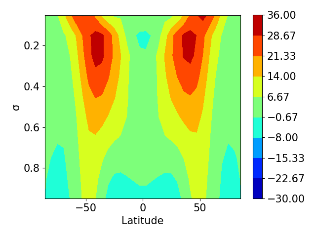
To perform the inversion, we set the prior . Within the algorithm, we assume that the observation error satisfies . All these Kalman inversions are initialized with , since initializing at the prior leads to unstable simulations at the first iteration. The bi-fidelity approach discussed in Subsection 3.2 is applied to speed up both UKI-1 and UKI-2. These forward model evaluations are computed on a T21 grid (triangular truncation at wavenumber 21, with points on the latitude-longitude transform grid) with 10 vertical levels equally spaced in (twice coarser in all three directions). They are abbreviated as UKI-1-BF and UKI-2-BF. The computational cost of the high-fidelity (T42) and low-fidelity (T21) models are about -CPU hour and -CPU hour, and therefore the bi-fidelity approach effectively reduces CPU costs. The 1000-day zonal mean of the temperature and velocity predicted by the low-resolution model with the truth parameters are shown in Fig. 13-bottom. It is worth mentioning there are significant discrepancies comparing with results computed on the T42 grid (Fig. 13-top). Whether these would be tolerable will depend on the use to which the posterior inference is put.
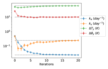
The estimated parameters and associated confidence intervals for each component at each iteration are depicted in Fig. 14. Since the prior covariance is large and the problem is over-determined it is natural to expect that the posterior mean should be close to the true parameters. Indeed all the different Kalman inversions, except UKI-1-BF (), do indeed converge to the true parameters.


5 Conclusion
Kalman-based inversion has been widely used to construct derivative-free optimization and sampling methods for nonlinear inverse problems. In this paper, we developed new Kalman-based inversion methods, for Bayesian inference and uncertainty quantification, which build on the work in both optimization and sampling. We propose a new method for Bayesian inference based on filtering a novel mean-field dynamical system subject to partial noisy observations, and which depends on the law of its own filtering distribution, together with application of the Kalman methodology. Theoretical guarantees are presented: for linear inverse problems, the mean and covariance obtained by the method converge exponentially fast to the posterior mean and covariance. For nonlinear inverse problems, numerical studies indicate the method delivers an excellent approximation of the posterior distribution for problems which are not too far from Gaussian. The methods are shown to be superior to existing coupling/transport methods, under the umbrella of iterative Kalman methods; and deterministic rather than stochastic implementations of Kalman methodology are found to be favorable. We further propose several simple strategies, including low-rank approximation and a bi-fidelity approach, to reduce the computational and memory cost of the proposed methodology.
There are numerous directions for future study in this area. On the theoretical side it would be of value to obtain theoretical guarantees concerning the accuracy of the methodology, when applied to nonlinear inverse problems, which are close to Gaussian. On the methodological side, it would be of particular interest to systematically quantify model-form error by using this framework, rather than to assume perfect the model scenario as we have done here.
Acknowledgments
AMS and DZH are supported by the generosity of Eric and Wendy Schmidt by recommendation of the Schmidt Futures program; AMS is also supported by the Office of Naval Research (ONR) through grant N00014-17-1-2079. JH is supported by the Simons Foundation as a Junior Fellow at New York University. SR is supported by Deutsche Forschungsgemeinschaft (DFG) - Project-ID 318763901 - SFB1294.
Appendix A Continuous Time Limit
To derive a continuous-time limit of the novel mean-field dynamical system (Eqs. 14, 15 and 18) we define and define by Then and . Let and be standard unit Brownian motions. Letting in (Eqs. 14, 15 and 18), we then obtain
| (75) | ||||
We are interested in the filtering problem of finding the distribution of given and then evaluating this distribution in the setting where defined in (17).
Under a similar limiting process, the Gaussian approximation algorithm defined by (22) becomes
| (76) | ||||
where , , and expectation is with respect to the distribution . Define , and note that [72, Lemma 2]. It follows that Eq. 76 can be rewritten as
| (77) | ||||
The stationary points of Eq. 77 satisfy
| (78) |
Although the plays no role in the continuous time limit, the original parameter does have a marked effect on discrete-time algorithms used in practice. To highlight this, we study the empirical effect of , in the context of the nonlinear 2-parameter model problem discussed in Section 4.3. The UKI-2 is applied with , , , , and . Empirically we observe that all solutions considered converge to approximately the same equilibrium point; but the convergence properties depend on The convergence of the posterior mean and covariance are reported in Fig. 15. The best convergence rate is achieved with around for this test. We note that the case also appears in [53] under the notion of ensemble transform Langevin dynamics.


Appendix B Iterative Kalman Filter
B.1 Gaussian Approximation
Iterative Kalman filters for inverse problems are obtained by applying filtering methods, over steps, to the dynamical system Eq. 12 with scaled observation error . Following the discussion in Subsection 2.2, the conceptual algorithm can be written as
| (79a) | ||||
| (79b) | ||||
where
| (80) |
and , the observation set at time . Different Kalman filters (See Subsection 2.4) can be applied, which lead to the IUKF, IEnKF, IEAKF and IETKF, all considered here. We have the following theorem about the convergence of the conceptual algorithm:
Theorem 2.
Related calculations in continuous time may be found in Section 2.2 of [75].
B.2 Gaussian Initialization
Theorem 2 can be extended to apply to the ensemble approximations of the mean field dynamics (79), provided that the initial ensemble represents the prior mean and covariance exactly. For iterative ensemble filters, we first sample (), and then correct them as follows.
Define
| (81) |
and correct with a matrix to keep zero mean and match the covariance
| (82) |
where
| (83) | ||||
References
References
- [1] Mrinal K Sen and Paul L Stoffa. Global optimization methods in geophysical inversion. Cambridge University Press, 2013.
- [2] Tapio Schneider, Shiwei Lan, Andrew Stuart, and Joao Teixeira. Earth system modeling 2.0: A blueprint for models that learn from observations and targeted high-resolution simulations. Geophysical Research Letters, 44(24):12–396, 2017.
- [3] Daniel Z Huang, Kailai Xu, Charbel Farhat, and Eric Darve. Learning constitutive relations from indirect observations using deep neural networks. Journal of Computational Physics, page 109491, 2020.
- [4] Kailai Xu, Daniel Z Huang, and Eric Darve. Learning constitutive relations using symmetric positive definite neural networks. Journal of Computational Physics, 428:110072, 2021.
- [5] Philip Avery, Daniel Z Huang, Wanli He, Johanna Ehlers, Armen Derkevorkian, and Charbel Farhat. A computationally tractable framework for nonlinear dynamic multiscale modeling of membrane woven fabrics. International Journal for Numerical Methods in Engineering, 122(10):2598–2625, 2021.
- [6] Brian H Russell. Introduction to seismic inversion methods. SEG Books, 1988.
- [7] Carey Bunks, Fatimetou M Saleck, S Zaleski, and G Chavent. Multiscale seismic waveform inversion. Geophysics, 60(5):1457–1473, 1995.
- [8] Tan Bui-Thanh, Omar Ghattas, James Martin, and Georg Stadler. A computational framework for infinite-dimensional Bayesian inverse problems. Part I: The linearized case, with application to global seismic inversion. SIAM Journal on Scientific Computing, 35(6):A2494–A2523, 2013.
- [9] James Martin, Lucas C Wilcox, Carsten Burstedde, and Omar Ghattas. A stochastic Newton MCMC method for large-scale statistical inverse problems with application to seismic inversion. SIAM Journal on Scientific Computing, 34(3):A1460–A1487, 2012.
- [10] LongLong Wang. Joint inversion of receiver function and surface wave dispersion based on innocent unscented kalman methodology. arXiv preprint arXiv:2202.09544, 2022.
- [11] Cristóbal Bertoglio, Philippe Moireau, and Jean-Frederic Gerbeau. Sequential parameter estimation for fluid–structure problems: Application to hemodynamics. International Journal for Numerical Methods in Biomedical Engineering, 28(4):434–455, 2012.
- [12] Philippe Moireau and Dominique Chapelle. Reduced-order unscented Kalman filtering with application to parameter identification in large-dimensional systems. ESAIM: Control, Optimisation and Calculus of Variations, 17(2):380–405, 2011.
- [13] Hrvoje Jasak, Aleksandar Jemcov, Zeljko Tukovic, et al. OpenFOAM: A C++ library for complex physics simulations. In International workshop on coupled methods in numerical dynamics, volume 1000, pages 1–20. IUC Dubrovnik Croatia, 2007.
- [14] Daniel Z Huang, Philip Avery, Charbel Farhat, Jason Rabinovitch, Armen Derkevorkian, and Lee D Peterson. Modeling, simulation and validation of supersonic parachute inflation dynamics during Mars landing. In AIAA Scitech 2020 Forum, page 0313, 2020.
- [15] Shunxiang Cao and Daniel Zhengyu Huang. Bayesian calibration for large-scale fluid structure interaction problems under embedded/immersed boundary framework. International Journal for Numerical Methods in Engineering, 2022.
- [16] Charles S Peskin. Numerical analysis of blood flow in the heart. Journal of computational physics, 25(3):220–252, 1977.
- [17] Daniel Z Huang, Dante De Santis, and Charbel Farhat. A family of position-and orientation-independent embedded boundary methods for viscous flow and fluid–structure interaction problems. Journal of Computational Physics, 365:74–104, 2018.
- [18] Marsha J Berger, Phillip Colella, et al. Local adaptive mesh refinement for shock hydrodynamics. Journal of computational Physics, 82(1):64–84, 1989.
- [19] Raunak Borker, Daniel Huang, Sebastian Grimberg, Charbel Farhat, Philip Avery, and Jason Rabinovitch. Mesh adaptation framework for embedded boundary methods for computational fluid dynamics and fluid-structure interaction. International Journal for Numerical Methods in Fluids, 90(8):389–424, 2019.
- [20] Nicolas Moës, John Dolbow, and Ted Belytschko. A finite element method for crack growth without remeshing. International journal for numerical methods in engineering, 46(1):131–150, 1999.
- [21] Zhihong Tan, Colleen M Kaul, Kyle G Pressel, Yair Cohen, Tapio Schneider, and João Teixeira. An extended eddy-diffusivity mass-flux scheme for unified representation of subgrid-scale turbulence and convection. Journal of Advances in Modeling Earth Systems, 10(3):770–800, 2018.
- [22] Ignacio Lopez-Gomez, Costa D Christopoulos, Haakon Ludvig Ervik, Oliver R Dunbar, Yair Cohen, and Tapio Schneider. Training physics-based machine-learning parameterizations with gradient-free ensemble kalman methods. 2022.
- [23] Charles J Geyer. Practical Markov chain Monte Carlo. Statistical science, pages 473–483, 1992.
- [24] Andrew Gelman, Walter R Gilks, and Gareth O Roberts. Weak convergence and optimal scaling of random walk Metropolis algorithms. The annals of applied probability, 7(1):110–120, 1997.
- [25] Jonathan Goodman and Jonathan Weare. Ensemble samplers with affine invariance. Communications in applied mathematics and computational science, 5(1):65–80, 2010.
- [26] Simon L Cotter, Gareth O Roberts, Andrew M Stuart, and David White. MCMC methods for functions: Modifying old algorithms to make them faster. Statistical Science, 28(3):424–446, 2013.
- [27] Pierre Del Moral, Arnaud Doucet, and Ajay Jasra. Sequential Monte Carlo samplers. Journal of the Royal Statistical Society: Series B (Statistical Methodology), 68(3):411–436, 2006.
- [28] Alexandros Beskos, Ajay Jasra, Ege A Muzaffer, and Andrew M Stuart. Sequential Monte Carlo methods for Bayesian elliptic inverse problems. Statistics and Computing, 25(4):727–737, 2015.
- [29] Jari Kaipio and Erkki Somersalo. Statistical and computational inverse problems, volume 160. Springer Science & Business Media, 2006.
- [30] Masoumeh Dashti and Andrew M Stuart. The Bayesian approach to inverse problems. arXiv preprint arXiv:1302.6989, 2013.
- [31] Masoumeh Dashti, Kody JH Law, Andrew M Stuart, and Jochen Voss. MAP estimators and their consistency in Bayesian nonparametric inverse problems. Inverse Problems, 29(9):095017, 2013.
- [32] James R Anderson and Carsten Peterson. A mean field theory learning algorithm for neural networks. Complex Systems, 1:995–1019, 1987.
- [33] Giorgio Parisi and Ramamurti Shankar. Statistical field theory. Physics Today, 41(12):110, 1988.
- [34] Manfred Opper and Cédric Archambeau. The variational Gaussian approximation revisited. Neural computation, 21(3):786–792, 2009.
- [35] Matias Quiroz, David J Nott, and Robert Kohn. Gaussian variational approximation for high-dimensional state space models. arXiv preprint arXiv:1801.07873, 2018.
- [36] Théo Galy-Fajou, Valerio Perrone, and Manfred Opper. Flexible and efficient inference with particles for the variational Gaussian approximation. Entropy, 23:990, 2021.
- [37] Danilo Rezende and Shakir Mohamed. Variational inference with normalizing flows. In International conference on machine learning, pages 1530–1538. PMLR, 2015.
- [38] Peter J Rossky, Jimmie D Doll, and Harold L Friedman. Brownian dynamics as smart Monte Carlo simulation. The Journal of Chemical Physics, 69(10):4628–4633, 1978.
- [39] Gareth O Roberts and Richard L Tweedie. Exponential convergence of Langevin distributions and their discrete approximations. Bernoulli, pages 341–363, 1996.
- [40] Jasper A Vrugt, CJF Ter Braak, CGH Diks, Bruce A Robinson, James M Hyman, and Dave Higdon. Accelerating Markov chain Monte Carlo simulation by differential evolution with self-adaptive randomized subspace sampling. International journal of nonlinear sciences and numerical simulation, 10(3):273–290, 2009.
- [41] Daniel Foreman-Mackey, David W Hogg, Dustin Lang, and Jonathan Goodman. EMCEE: The MCMC hammer. Publications of the Astronomical Society of the Pacific, 125(925):306, 2013.
- [42] Benedict Leimkuhler, Charles Matthews, and Jonathan Weare. Ensemble preconditioning for Markov chain Monte Carlo simulations. Stat. Comput., 28:277–290, 2018.
- [43] Adrian Smith. Sequential Monte Carlo methods in practice. Springer Science & Business Media, 2013.
- [44] Geir Evensen. The ensemble Kalman filter for combined state and parameter estimation. IEEE Control Systems Magazine, 29(3):83–104, 2009.
- [45] Sebastian Reich and Colin Cotter. Probabilistic forecasting and Bayesian data assimilation. Cambridge University Press, 2015.
- [46] Kody Law, Andrew Stuart, and Kostas Zygalakis. Data assimilation. Cham, Switzerland: Springer, 2015.
- [47] Sebastian Reich. A dynamical systems framework for intermittent data assimilation. BIT Numerical Mathematics, 51(1):235–249, 2011.
- [48] Tarek A El Moselhy and Youssef M Marzouk. Bayesian inference with optimal maps. Journal of Computational Physics, 231(23):7815–7850, 2012.
- [49] Sebastian Reich. A nonparametric ensemble transform method for Bayesian inference. SIAM Journal on Scientific Computing, 35(4):A2013–A2024, 2013.
- [50] Youssef Marzouk, Tarek Moselhy, Matthew Parno, and Alessio Spantini. Sampling via measure transport: An introduction. Handbook of uncertainty quantification, pages 1–41, 2016.
- [51] José A Carrillo, Young-Pil Choi, Claudia Totzeck, and Oliver Tse. An analytical framework for consensus-based global optimization method. Mathematical Models and Methods in Applied Sciences, 28(06):1037–1066, 2018.
- [52] JA Carrillo, F Hoffmann, AM Stuart, and U Vaes. Consensus-based sampling. Studies in Applied Mathematics, 2021.
- [53] Jakiw Pidstrigach and Sebastian Reich. Affine-invariant ensemble transform methods for logistic regression. arXiv preprint arXiv:2104.08061, 2021.
- [54] Alexandre A Emerick and Albert C Reynolds. Investigation of the sampling performance of ensemble-based methods with a simple reservoir model. Computational Geosciences, 17(2):325–350, 2013.
- [55] Yan Chen and Dean S Oliver. Ensemble randomized maximum likelihood method as an iterative ensemble smoother. Mathematical Geosciences, 44(1):1–26, 2012.
- [56] Marco A Iglesias, Kody JH Law, and Andrew M Stuart. Ensemble Kalman methods for inverse problems. Inverse Problems, 29(4):045001, 2013.
- [57] Eric A Wan and Rudolph Van Der Merwe. The unscented Kalman filter for nonlinear estimation. In Proceedings of the IEEE 2000 Adaptive Systems for Signal Processing, Communications, and Control Symposium (Cat. No. 00EX373), pages 153–158. Ieee, 2000.
- [58] Rudolph Emil Kalman. A new approach to linear filtering and prediction problems. J. Basic Eng. Mar, 82(1):35–45, 1960.
- [59] Harold Wayne Sorenson. Kalman filtering: Theory and application. IEEE, 1985.
- [60] Andrew H Jazwinski. Stochastic processes and filtering theory. Courier Corporation, 2007.
- [61] Geir Evensen. Sequential data assimilation with a nonlinear quasi-geostrophic model using Monte Carlo methods to forecast error statistics. Journal of Geophysical Research: Oceans, 99(C5):10143–10162, 1994.
- [62] Jeffrey L Anderson. An ensemble adjustment Kalman filter for data assimilation. Monthly weather review, 129(12):2884–2903, 2001.
- [63] Craig H Bishop, Brian J Etherton, and Sharanya J Majumdar. Adaptive sampling with the ensemble transform Kalman filter. Part I: Theoretical aspects. Monthly weather review, 129(3):420–436, 2001.
- [64] Simon J Julier, Jeffrey K Uhlmann, and Hugh F Durrant-Whyte. A new approach for filtering nonlinear systems. In Proceedings of 1995 American Control Conference-ACC’95, volume 3, pages 1628–1632. IEEE, 1995.
- [65] Michael K Tippett, Jeffrey L Anderson, Craig H Bishop, Thomas M Hamill, and Jeffrey S Whitaker. Ensemble square root filters. Monthly Weather Review, 131(7):1485–1490, 2003.
- [66] Marc Bocquet and Pavel Sakov. Joint state and parameter estimation with an iterative ensemble Kalman smoother. Nonlinear Processes in Geophysics, 20(5):803–818, 2013.
- [67] Sangeetika Ruchi, Svetlana Dubinkina, and MA Iglesias. Transform-based particle filtering for elliptic Bayesian inverse problems. Inverse Problems, 35(11):115005, 2019.
- [68] Marco Iglesias and Yuchen Yang. Adaptive regularisation for ensemble Kalman inversion. Inverse Problems, 37(2):025008, 2021.
- [69] MY Matveev, A Endruweit, AC Long, MA Iglesias, and MV Tretyakov. Bayesian inversion algorithm for estimating local variations in permeability and porosity of reinforcements using experimental data. Composites Part A: Applied Science and Manufacturing, 143:106323, 2021.
- [70] Chak-Hau Michael Tso, Marco Iglesias, Paul Wilkinson, Oliver Kuras, Jonathan Chambers, and Andrew Binley. Efficient multiscale imaging of subsurface resistivity with uncertainty quantification using ensemble Kalman inversion. Geophysical Journal International, 225(2):887–905, 2021.
- [71] Neil K Chada, Andrew M Stuart, and Xin T Tong. Tikhonov regularization within ensemble Kalman inversion. SIAM Journal on Numerical Analysis, 58(2):1263–1294, 2020.
- [72] Daniel Z Huang, Tapio Schneider, and Andrew M Stuart. Unscented Kalman inversion. arXiv preprint arXiv:2102.01580, 2021.
- [73] Simon Weissmann, Neil Kumar Chada, Claudia Schillings, and Xin Thomson Tong. Adaptive Tikhonov strategies for stochastic ensemble Kalman inversion. Inverse Problems, 2022.
- [74] Oliver G Ernst, Björn Sprungk, and Hans-Jörg Starkloff. Analysis of the ensemble and polynomial chaos Kalman filters in Bayesian inverse problems. SIAM/ASA Journal on Uncertainty Quantification, 3(1):823–851, 2015.
- [75] Alfredo Garbuno-Inigo, Franca Hoffmann, Wuchen Li, and Andrew M Stuart. Interacting Langevin diffusions: Gradient structure and ensemble Kalman sampler. SIAM Journal on Applied Dynamical Systems, 19(1):412–441, 2020.
- [76] Alfredo Garbuno-Inigo, Nikolas Nüsken, and Sebastian Reich. Affine invariant interacting Langevin dynamics for Bayesian inference. SIAM Journal on Applied Dynamical Systems, 19(3):1633–1658, 2020.
- [77] Nikolas Nüsken and Sebastian Reich. Note on interacting Langevin diffusions: Gradient structure and ensemble Kalman sampler by Garbuno-Inigo, Hoffmann, Li and Stuart. arXiv preprint arXiv:1908.10890, 2019.
- [78] Daniel Sanz-Alonso, Andrew M Stuart, and Armeen Taeb. Inverse problems and data assimilation. arXiv preprint arXiv:1810.06191, 2018.
- [79] Edoardo Calvello, Sebastian Reich, and Andrew M Stuart. Ensemble Kalman methods: A mean field perspective. arXiv preprint arXiv:TBD, 2022.
- [80] Peter Lancaster and Leiba Rodman. Algebraic Riccati equations. Clarendon press, 1995.
- [81] Philippe Bougerol. Kalman filtering with random coefficients and contractions. SIAM Journal on Control and Optimization, 31(4):942–959, 1993.
- [82] Simon J Julier and Jeffrey K Uhlmann. Reduced sigma point filters for the propagation of means and covariances through nonlinear transformations. In Proceedings of the 2002 American Control Conference (IEEE Cat. No. CH37301), volume 2, pages 887–892. IEEE, 2002.
- [83] Geir Evensen. Data assimilation: The ensemble Kalman filter. Springer Science & Business Media, 2009.
- [84] Xuguang Wang and Craig H Bishop. A comparison of breeding and ensemble transform Kalman filter ensemble forecast schemes. Journal of the atmospheric sciences, 60(9):1140–1158, 2003.
- [85] Jeffrey L Anderson. An adaptive covariance inflation error correction algorithm for ensemble filters. Tellus A: Dynamic meteorology and oceanography, 59(2):210–224, 2007.
- [86] Yan Chen and Dean S Oliver. Localization and regularization for iterative ensemble smoothers. Computational Geosciences, 21(1):13–30, 2017.
- [87] Roger G Ghanem and Pol D Spanos. Stochastic finite elements: a spectral approach. Courier Corporation, 2003.
- [88] Andrew M Stuart. Inverse problems: A Bayesian perspective. Acta numerica, 19:451–559, 2010.
- [89] Martin Ehrendorfer. Spectral numerical weather prediction models. SIAM, 2011.
- [90] Paul G Constantine, Eric Dow, and Qiqi Wang. Active subspace methods in theory and practice: applications to Kriging surfaces. SIAM Journal on Scientific Computing, 36(4):A1500–A1524, 2014.
- [91] Tiangang Cui, James Martin, Youssef M Marzouk, Antti Solonen, and Alessio Spantini. Likelihood-informed dimension reduction for nonlinear inverse problems. Inverse Problems, 30(11):114015, 2014.
- [92] Tiangang Cui and Xin T Tong. A unified performance analysis of likelihood-informed subspace methods. arXiv preprint arXiv:2101.02417, 2021.
- [93] Stefan Heinrich. Multilevel Monte Carlo methods. In International Conference on Large-Scale Scientific Computing, pages 58–67. Springer, 2001.
- [94] Michael B Giles. Multilevel Monte Carlo methods. Acta Numerica, 24:259–328, 2015.
- [95] Han Gao and Jian-Xun Wang. A bi-fidelity ensemble Kalman method for PDE-constrained inverse problems in computational mechanics. Computational Mechanics, 67(4):1115–1131, 2021.
- [96] Hillary R Fairbanks, Lluís Jofre, Gianluca Geraci, Gianluca Iaccarino, and Alireza Doostan. Bi-fidelity approximation for uncertainty quantification and sensitivity analysis of irradiated particle-laden turbulence. Journal of Computational Physics, 402:108996, 2020.
- [97] Håkon Hoel, Kody JH Law, and Raul Tempone. Multilevel ensemble kalman filtering. SIAM Journal on Numerical Analysis, 54(3):1813–1839, 2016.
- [98] Neil K Chada, Ajay Jasra, and Fangyuan Yu. Multilevel ensemble kalman-bucy filters. SIAM/ASA Journal on Uncertainty Quantification (Accepted), arXiv preprint arXiv:2011.04342, 2020.
- [99] David J Albers, Paul-Adrien Blancquart, Matthew E Levine, Elnaz Esmaeilzadeh Seylabi, and Andrew Stuart. Ensemble Kalman methods with constraints. Inverse Problems, 35(9):095007, 2019.
- [100] Neil K Chada, Claudia Schillings, and Simon Weissmann. On the incorporation of box-constraints for ensemble kalman inversion. arXiv preprint arXiv:1908.00696, 2019.
- [101] Tapio Schneider, Andrew M Stuart, and Jin-Long Wu. Ensemble Kalman inversion for sparse learning of dynamical systems from time-averaged data. arXiv preprint arXiv:2007.06175, 2020.
- [102] Michael Herty and Giuseppe Visconti. Kinetic methods for inverse problems. arXiv preprint arXiv:1811.09387, 2018.
- [103] René Pinnau, Claudia Totzeck, Oliver Tse, and Stephan Martin. A consensus-based model for global optimization and its mean-field limit. Mathematical Models and Methods in Applied Sciences, 27(01):183–204, 2017.
- [104] JA Carrillo, C Totzeck, and U Vaes. Consensus-based optimization and ensemble Kalman inversion for global optimization problems with constraints. arXiv preprint arXiv:2111.02970, 2021.
- [105] José A Carrillo, Shi Jin, Lei Li, and Yuhua Zhu. A consensus-based global optimization method for high dimensional machine learning problems. ESAIM: Control, Optimisation and Calculus of Variations, 27:S5, 2021.
- [106] Mark Asch, Marc Bocquet, and Maëlle Nodet. Data assimilation: Methods, algorithms, and applications. SIAM, 2016.
- [107] Dean S Oliver, Albert C Reynolds, and Ning Liu. Inverse theory for petroleum reservoir characterization and history matching. Cambridge University Press, 2008.
- [108] Zhiyan Ding, Qin Li, and Jianfeng Lu. Ensemble Kalman inversion for nonlinear problems: Weights, consistency, and variance bounds. arXiv preprint arXiv:2003.02316, 2020.
- [109] Isaac M Held and Max J Suarez. A proposal for the intercomparison of the dynamical cores of atmospheric general circulation models. Bulletin of the American Meteorological society, 75(10):1825–1830, 1994.