GSVD for Kronecker Products in regularizationSweeney, Español, and Renaut
Efficient Decomposition-Based Algorithms for -Regularized Inverse Problems with Column-Orthogonal and Kronecker Product Matrices
Abstract
We consider an -regularized inverse problem where both the forward and regularization operators have a Kronecker product structure. By leveraging this structure, a joint decomposition can be obtained using generalized singular value decompositions. We show how this joint decomposition can be effectively integrated into the Split Bregman and Majorization-Minimization methods to solve the -regularized inverse problem. Furthermore, for cases involving column-orthogonal regularization matrices, we prove that the joint decomposition can be derived directly from the singular value decomposition of the system matrix. As a result, we show that framelet and wavelet operators are efficient for these decomposition-based algorithms in the context of -regularized image deblurring problems.
keywords:
regularization, Kronecker product, Framelets, Wavelets, Generalized singular value decomposition65F22, 65F10, 68W40
1 Introduction
We are interested in solving discrete ill-posed inverse problems of the form , where , , , and . It is assumed that the matrix has full column rank but is ill-conditioned, and is contaminated by additive Gaussian noise: , where is a Gaussian noise vector. Throughout this paper, we normalize the problem by dividing and by the standard deviation of . This corresponds to whitening the noise in the data. Due to the ill-posedness of this problem, the solution of the normal equations, , is poor, and therefore, we will apply regularization. With generalized Tikhonov regularization [48], is selected to solve the minimization problem
| (1) |
where is a regularization parameter and is a regularization matrix. is often selected as the discretization of some derivative operator [28]. We also assume that
| (2) |
where denotes the null space of the matrix .
Instead of considering the Tikhonov problem Eq. 1, we will consider a sparsity-preserving problem
| (3) |
where is a regularization parameter. We will solve Eq. 3 using two iterative methods, split Bregman (SB) [24] and Majorization-Minimization (MM) [31, 32]. Both methods share a minimization sub-problem of the same form [47].
Our focus is on Kronecker Product (KP) matrices and , that is, matrices that can be written as and where denotes the Kronecker product, which is defined for matrices and by
| (4) |
Thus, we are interested in solving problem Eq. 3 of the specific form
| (5) |
KP matrices and arise in many applications. In image deblurring problems, is a KP matrix, provided that the blur can be separated in the horizontal and vertical directions [29]. Another case where is a KP matrix is in 2D nuclear magnetic resonance (NMR) problems [6, 23], where the goal is to reconstruct a map of relaxation times from a probed material. is a KP matrix with certain forms of regularization, such as when orthonormal framelets [44] or wavelets [12] are used in two dimensions. Both are tight frames, namely, they form redundant orthogonal bases for . This redundancy allows for robust representations where the loss of information is more tolerable [11]. When used as regularization in Eq. 3, framelet [8, 10, 11, 54] and wavelet-based [18] methods enforce sparsity on the solution within the tight frame.
In [8], tight frames are used for regularization in a general - problem without the assumptions of having KP matrices. Other minimization problems with KP matrices or have been studied before. Least-squares problems of the form
have been solved efficiently using the singular value and QR decompositions [19, 20]. The special case where the forward operator has the form , which is equivalent to a matrix inverse problem, has also been analyzed [26]. For least-squares problems of the form
| (6) |
the generalized singular value decompositions (GSVDs) of and can be used to obtain a joint decomposition and solve the problem [3, 35, 52]. In particular, Givens rotations can be used to diagonalize the matrix containing the generalized singular values, which then diagonalizes the problem. A regularized problem of the form
| (7) |
occurs in adaptive optics [3, 35]. The structure of this problem can be utilized to rewrite it as a least-squares problem with a preconditioner. Another problem that utilizes KP matrices is the constrained least-squares problem
which is considered in [4]. In this case, both the forward operator and the constraint are KP matrices, and a null space method can be applied to the matrix equations. The solution is unique under certain circumstances, which can be analyzed using the GSVD [4].
In cases where is not a KP matrix, there are methods to approximate it by a Kronecker product so that the benefits of the KP structure can still be utilized. The nearest Kronecker product can be found by minimizing
Van Loan and Pitsianis [53] developed a method for solving this problem, and in [42], Pitsianis extended it to solve the problem
These KP approximations have been applied to the forward matrix in imaging problems [7, 22, 33, 34].
Main Contributions: We utilize joint decompositions that exploit the KP structure, computed at the first iteration only, to solve Eq. 5 with SB and MM where the regularization parameter is selected at each iteration as in [47]. We introduce a family of regularization operators that are column orthogonal. This family includes framelet and wavelet matrices. We show that with these matrices, we can obtain the GSVDs needed for the joint decompositions directly from the singular value decompositions (SVDs) of and , allowing us to use framelets and wavelets without computing a GSVD. Other regularization matrices, such as finite-difference operators, would require computing GSVDs to implement these same decomposition-based algorithms. This makes using framelet and wavelet operators efficient for solving -regularized problems with SB and MM. We also show that the solution of the generalized Tikhonov problem with a fixed regularization parameter will generate the same solution using framelets and wavelets.
This paper is organized as follows. In Section 2, we review two iterative methods for solving Eq. 3, split Bregman and Majorization-Minimization. In Section 3, the GSVD is presented and we discuss how it can be used to obtain a joint decomposition that can then be utilized within the iterative methods. Theoretical results are also presented for when and are column orthogonal, which allow this joint decomposition to be obtained from the SVD rather than the GSVD. In Section 4, we introduce a family of column-orthogonal regularization operators that include the framelet and wavelet regularization matrices. The iterative methods are then tested on image deblurring examples in Section 5. Although the results presented in Section 3 apply to a general , the examples are presented for cases with . Conclusions are presented in Section 6.
2 Iterative techniques for solution of the sparsity constrained problem
In this section, we will consider solving Eq. 3 using two iterative methods: the split Bregman (SB) method and the Majorization-Minimization (MM) method. Both methods only require computing two GSVDs, which can be reused for every iteration.
2.1 Split Bregman
The SB method was first introduced by Goldstein and Osher [24]. This method rewrites Eq. 3 as a constrained optimization problem
| (8) |
which can then be converted to the unconstrained optimization problem
| (9) |
This unconstrained optimization problem can be solved through a series of minimization steps and updates, here indicated by superscripts for iteration , known as the SB iteration
| (10) | ||||
| (11) |
In Eq. 10, the vectors and can be found separately as
| (12) | ||||
| (13) |
Here, and in the update Eq. 11, is the vector of Lagrange multipliers. Defining , Eq. 13 becomes
| (14) |
Since the elements of are decoupled in Eq. 14, can be computed using shrinkage operators. Consequently, each element is given by
where . We will also select the parameter at each iteration by applying parameter selection methods to Eq. 12 as in [47]. We terminate iterations once the relative change in the solution , defined as
| (15) |
drops below a specified tolerance or after a specified maximum number of iterations is reached. The SB algorithm is summarized in Algorithm 1. Notice that SB is related to applying the alternating direction method of multipliers (ADMM) to the augmented Lagrangian in Eq. 9 [17].
2.2 Majorization-Minimization
The MM method is another iterative method for solving Eq. 3. It is an optimization method that utilizes two steps: majorization and minimization [32]. First, in the majorization step, the function is majorized with a surrogate convex function. The convexity of this function is then utilized in the minimization step. When applied to Eq. 3, MM is often combined with the generalized Krylov subspace (GKS) method [9, 31, 41] to solve large-scale problems. In this method, known as MM-GKS, the Krylov subspace is enlarged at each iteration, and MM is then applied to the problem in the subspace. In this paper, we will apply the MM method directly to Eq. 3 instead of building a Krylov subspace. For the majorant, we will use the fixed quadratic majorant from [31]. There are other ways for majorizing Eq. 3 as well, including both fixed and adaptive quadratic majorants [1, 9, 41].
The fixed majorant in [31] depends on a parameter . With this fixed majorant, the minimization problem at the iteration is
| (16) |
where and
| (17) |
with . All operations in Eq. 17 are component-wise. As in [47], we will consider selecting the parameter at each iteration using the minimization in Eq. 16. The iterations are again terminated when drops below a specified tolerance or after iterations are reached. The MM algorithm is summarized in Algorithm 2.
2.3 Parameter Selection Methods
In both iterative methods, we will solve a minimization problem of the form
| (18) |
at each iteration. To select , we will use both generalized cross validation (GCV) and the degrees of freedom (dof) test as discussed in the context of application to SB and MM algorithms in [47]. GCV [2, 25] selects to minimize the average predictive risk when an entry of is left out. This method does not require any information about the noise. We will follow [47] in which the GCV is extended to this inner minimization problem.
The dof test [37, 38, 43] is a statistical test that treats as a random variable with mean and utilizes information about the noise to select . Under the assumption that is normally distributed with mean and covariance matrix , denoted , and , the functional
follows a distribution with dof [47]. The dof test then selects so that most resembles this distribution. As an approximation of , we will use as in [47]. In this case, the determination of is implemented efficiently as a one-dimensional root-finding algorithm. On the other hand, if is not the mean of , then instead follows a non-central distribution [43] and a non-central test can be applied in a similar, but more difficult manner to select .
3 Solving Generalized Tikhonov with Kronecker Product Matrices
Under the assumption that both and are KP matrices, we can solve the minimization problem Eq. 18 occurring for both the SB and MM methods by using a joint decomposition resulting from the individual GSVDs of and . The GSVD is a joint decomposition of a matrix pair introduced by Van Loan [51]. It has been formulated in different ways [30, 39], but for this paper, we use the definition of the GSVD given in [30].
Lemma 3.1.
For and , let . Let , , and . Then, there exist orthogonal matrices , , , and , and non-singular matrix such that
| (19) |
where and with
| (20a) | ||||
| (20b) | ||||
| (20c) | ||||
| (20d) | ||||
Here the identity matrices are and the zero matrices are The singular values of are the nonzero singular values of . Defining
then and , where has full column rank. If , then is invertible and we have that and , where .
The ratios in the GSVD are known as the generalized singular values (GSVs) [27] and are sorted in decreasing order in Lemma 3.1. If and , then the corresponding GSV is infinite. The columns of that correspond to span while the columns of that correspond to span .
From the GSVDs of the factors and ,
| (21) |
we can construct a joint decomposition of and using the properties of the Kronecker product [52]. This joint decomposition is given by
| (22) |
Let us assume, without loss of generality, that is square, meaning that , where is an operator that reshapes the vector into an matrix. We will also assume that have at least as many rows as columns. With assumption Eq. 2, in Lemma 3.1 and the solution to Eq. 18 is then given as
| (23) |
Since , , , and are invertible, and we may set and . Let and be the first columns of and , respectively, and let and be the last columns of and , respectively. Define also and , where and . Then, using Eq. 22 and
| (24) |
where is the vectorization of the matrix , the solution in Eq. 23 can be written as
| (25) |
where denotes element-wise multiplication and and are given by
Here, and refer to the (potentially) non-zero entry in column of or .
In both SB and MM, must also be computed at each iteration. This computation can be written using Eq. 24 as
| (26) |
where .
In the dof test, we also compute . Defining by
and , we have that
| (27) |
Notice that Eq. 25, Eq. 26, and Eq. 27 allow each step in the iterative methods to be computed using only the individual GSVDs in Eq. 21.
3.1 Theoretical Properties of the GSVD of Column-Orthogonal Matrices
Here, we examine the properties of the GSVD of a matrix pair where one is a column-orthogonal matrix. We refer to a matrix , , as column orthogonal if . First, we recall the singular value decomposition (SVD) of . The SVD is a decomposition of the form , where and are orthogonal and is diagonal with entries and . These diagonal entries are known as the singular values (SVs) of and are sorted in decreasing order: . The rank of is equal to the number of non-zero SVs. It is well known that when , the GSVD of reduces to the SVD of with , where the are sorted in decreasing order [45, 50]. If has full column rank, the GSVs are the SVs of [14, 15, 36, 56]. If, however, is column orthogonal, we can say more about the GSVD of as described by the following lemma.
Lemma 3.2.
Let be column orthogonal and . Then, in the GSVD of , for and for . Further, , where . The are sorted in decreasing order as in Lemma 3.1.
Proof 3.3.
Let be the rank of and let the SVD of be given by . Since is orthogonal, we can write that . This provides a joint decomposition of the form
| (28) |
Since is invertible, we have that
| (29) |
where , , and . With this,
Hence, Eq. 20d is satisfied. is orthogonal from the SVD and is column orthogonal since is column orthogonal and is orthogonal. is not necessarily orthogonal since may have more rows than columns. In this case, we add columns to the left of to make it orthogonal. To maintain the decomposition, we also add rows of zeros to the top of that correspond to these additional columns in . Following this, the decomposition is then a GSVD.
Notice that the GSVs for are
and for are . Thus, if , the GSVs are the SVs of . If , then the GSVs for come from the columns of zeros in and are . From Eq. 29, we can also see that is from the SVD of with scaled columns. In particular, the scaling implies that for , and . This also shows that is related to and, by extension, to , since .
If is column orthogonal instead of , we obtain a similar result by flipping the roles of and and writing a decomposition of in terms of the SVD of . In this case, the SVD of determines the matrices in the GSVD of . On the other hand, if is column orthogonal, then and the system of equations is not ill-posed. Thus, we immediately obtain , and we do not need the GSVD.
To obtain the same result as in Lemma 3.2, we can also consider the generalized eigenvalue problem [40] involving the matrix pair , in which the goal is to find a scalar and non-zero vector such that
| (30) |
where are symmetric. When is column orthogonal, Eq. 30 simplifies to the eigenvalue problem
| (31) |
Lemma 3.4.
Proof 3.5.
Since is positive definite, there exists a solution to Eq. 30 and any and that solve Eq. 30 are real [21, 40]. The is a generalized eigenvalue and is the associated eigenvector. We can write Eq. 30 to include all eigenvalues and eigenvectors as a matrix equation
| (32) |
where contains the generalized eigenvectors and is a diagonal matrix with the generalized eigenvalues. When is column orthogonal, Eq. 30 simplifies to the eigenvalue problem for :
Thus, the eigenvalues of are the eigenvalues of , meaning that the generalized eigenvalues of are the eigenvalues of . The associated eigenvectors for are the columns of , which are also the generalized eigenvectors of from Eq. 32. When , this analysis can be connected back to the GSVs. Since the SVs of are the square roots of the eigenvalues of and the finite GSVs of are the square roots of the finite generalized eigenvalues of [5], the GSVs of are the SVs of .
From the proof of Lemma 3.2, we can see that when is column orthogonal, the GSVD of can be obtained from the SVD of . This means that instead of computing the GSVD, we can use the SVD of . Another result of Lemma 3.2 is that the basis for the solution of Eq. 18 is determined solely by the right singular vectors of and not by . Similarly, the GSVs are also determined by the SVs of . The only matrix in the GSVD that changes between the framelets and wavelets is the matrix, which is used in the solution Eq. 25 when . When though, as in the generalized Tikhonov problem Eq. 1, both will produce the same solution, leading to the following corollary.
Corollary 3.6.
Let and both be column orthogonal. Then, for a given , it makes no difference whether or is used as the regularization matrix for the generalized Tikhonov problem Eq. 1 as the problem reduces to standard Tikhonov with for both matrices. Thus, the solutions will be the same, to machine precision.
4 Family of Regularization Operators
This section presents a family of regularization operators , which we adopted for the solution of Eq. 3. Specifically, we will consider a two-level framelet analysis operator [13, 44] and the Daubechies D4 discrete wavelet transform [12].
Consider a matrix that corresponds to a one-dimensional (1D) transform of the form
and its two-dimensional (2D) transform consists of the form
where for This then yields the 2D-transform-regularized problem
| (34) |
To solve Eq. 34 we observe that , where is a permutation matrix. Since
for any permutation matrix , we have that
As a result, solving
| (35) |
is equivalent to solving Eq. 34. Thus, we will solve Eq. 35 as it provides the advantage of the KP structure.
4.1 Framelets
Following the presentation in [8], we use tight frames that are determined by B-splines for regularization. With these frames, we have one low-pass filter and two high pass filters given by
The one-dimensional operator is given by
Since we are concerned with image deblurring in two dimensions, the two-dimensional operator is then constructed using the Kronecker product:
The matrix is a low-pass filter, while each of the other matrices contains at least one of the high-pass filters. The 2D operator , obtained by the concatenation of these matrices, is given by
4.2 Wavelets
Discrete wavelet transforms are composed of a low-pass filter, and a high-pass filter, [16, 49]. For a discrete wavelet transform of order , let be the filter coefficients. Then, the filter matrices have the forms
where . The 1D DWT matrix is then
As with the framelets, the 2D operator is constructed by taking the Kronecker products of the low-pass and high-pass filters:
The 2D operator is then
For the examples, we will use the D4 wavelet transform, which is of order 4 and has the filter coefficients
5 Numerical Results
In this section, the SB and MM methods are applied to image deblurring examples where the blur is separable. For the blurring matrix , we consider , , , to be a one-dimensional blur with either zero or periodic boundary conditions. With zero boundary conditions, is a symmetric Toeplitz matrix with the first row
while with periodic boundary conditions, is a circulant matrix with first row
Here, and are blur parameters. We then add Gaussian noise to according to a specified blurred signal to noise ratio (BSNR), which is defined as
The image is then deblurred using the SB and MM methods, with being defined by framelets or wavelets as described in Section 4. We set set and . The methods are compared using the relative error (RE) defined by
and the improved signal to noise ratio (ISNR), which is defined by
Both metrics measure the quality of the solution, with a smaller RE and a larger ISNR indicating a better solution.
5.1 Blurring Examples


5.1.1 Example 1
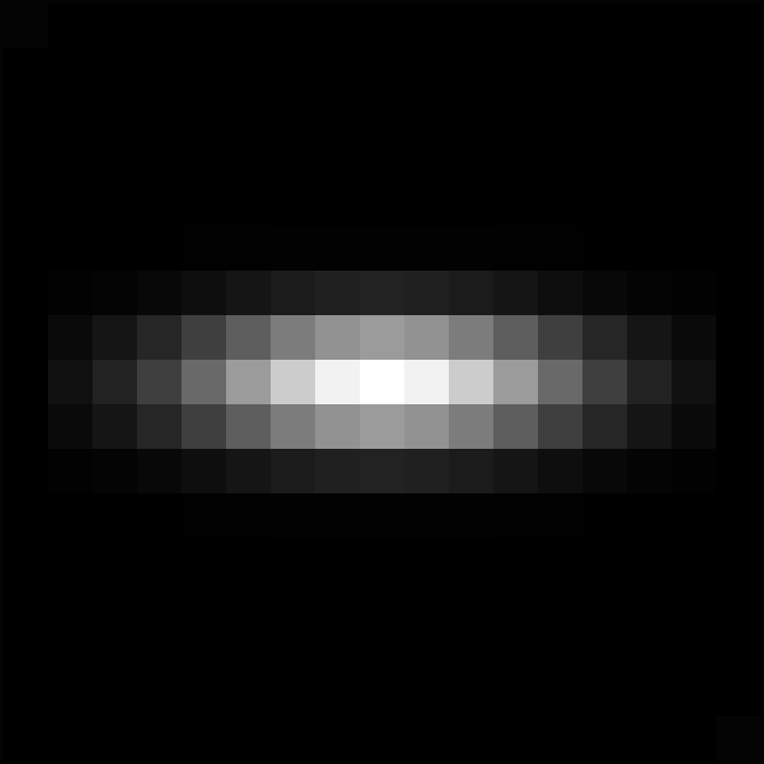
For the first example, we blur the satellite image in Fig. 1(a) with size . For , we use zero boundary conditions, , , and . The corresponding point spread function (PSF) is shown in Fig. 1(b), and the blurred image is shown in Fig. 1(c). Gaussian noise with is added to obtain as seen in Fig. 1(d). This problem is then solved using SB with and MM with . The solutions in Fig. 2 show that framelet regularization produces solutions with fewer artifacts in the background. The RE and ISNR for these methods are shown in Fig. 3. This shows that SB and MM perform similarly and that the framelet solutions have larger ISNRs than the wavelet solutions. The results are summarized in Table 1 along with timing. From this, we can observe that with , wavelet methods converge faster than framelet methods while with GCV, framelet methods converge faster. In all cases, the selection method, which is a root-finding technique, is faster than GCV despite GCV taking fewer iterations to converge. GCV and produce solutions with comparable RE and ISNR with either framelets or wavelets.


| Method | RE | ISNR | Iterations | Timing (s) |
|---|---|---|---|---|
| SB Framelets, Optimal | 0.26 | 35.0 | 9 | — |
| SB Framelets, GCV | 0.26 | 34.7 | 8 | 0.17 |
| SB Framelets, | 0.26 | 34.9 | 10 | 0.08 |
| SB Wavelets, Optimal | 0.28 | 34.2 | 11 | — |
| SB Wavelets, GCV | 0.28 | 34.2 | 9 | 0.21 |
| SB Wavelets, | 0.28 | 34.2 | 13 | 0.04 |
| MM Framelets, Optimal | 0.28 | 34.3 | 8 | — |
| MM Framelets, GCV | 0.29 | 34.4 | 6 | 0.13 |
| MM Framelets, | 0.27 | 34.5 | 8 | 0.08 |
| MM Wavelets, Optimal | 0.28 | 34.1 | 11 | — |
| MM Wavelets, GCV | 0.28 | 34.2 | 10 | 0.17 |
| MM Wavelets, | 0.28 | 34.1 | 14 | 0.05 |
5.1.2 Example 2
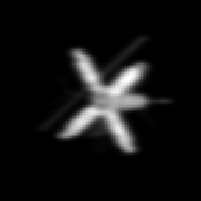
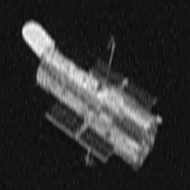
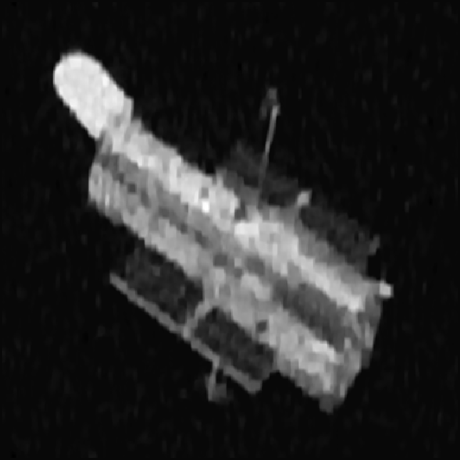
As a larger example, we blur the image of the Hubble telescope in Fig. 4(a) which has size . Here, we use zero boundary conditions, , , and . Gaussian noise with is added to the blurred image to produce . The PSF, , and are shown in Fig. 4. We solve this problem using SB with and MM with . The solutions are shown in Fig. 5 with the RE and ISNR in Fig. 6. When comparing RE and ISNR, SB and MM perform similarly for both framelets and wavelets. We observe that framelets produce solutions with slightly smaller REs and larger ISNRs than wavelets. With wavelets, the test does not perform as well as GCV, but with framelets, both GCV and achieve solutions near the optimal. The results are summarized in Table 2 along with timing. From this, we can see that although the framelet methods produce better solutions, they take longer than wavelet methods to run. We also observe again that the selection method is faster than GCV, that again takes fewer iterations.


| Method | RE | ISNR | Iterations | Timing (s) |
|---|---|---|---|---|
| SB Framelets, Optimal | 0.23 | 32.9 | 8 | — |
| SB Framelets, GCV | 0.23 | 32.9 | 8 | 4.76 |
| SB Framelets, | 0.23 | 33.0 | 14 | 2.75 |
| SB Wavelets, Optimal | 0.24 | 32.6 | 8 | — |
| SB Wavelets, GCV | 0.25 | 32.3 | 7 | 3.29 |
| SB Wavelets, | 0.30 | 30.7 | 14 | 1.14 |
| MM Framelets, Optimal | 0.24 | 32.7 | 6 | — |
| MM Framelets, GCV | 0.23 | 32.9 | 6 | 4.22 |
| MM Framelets, | 0.23 | 32.8 | 10 | 2.81 |
| MM Wavelets, Optimal | 0.24 | 32.6 | 7 | — |
| MM Wavelets, GCV | 0.25 | 32.4 | 7 | 3.89 |
| MM Wavelets, | 0.29 | 30.9 | 16 | 1.65 |
5.1.3 Example 3
Now, we consider the barcode image in Fig. 7(a), which has size . Here, we use periodic boundary conditions for the blurring matrix along with parameters , , and . Gaussian noise with is added to the blurred image to obtain . The PSF, , and are shown in Fig. 7. For this problem, we will compare regularization using column-orthogonal matrices with regularization using the first derivative operator in one direction. For this derivative operator, we use periodic boundary conditions, which gives a matrix of the form , where is given by
This matrix only captures the derivative in the horizontal direction, which fits well with this example. We solve this problem using SB and MM where in SB and in MM.
The results for framelets and are shown in Fig. 8 with the RE and ISNR plotted in Fig. 9. Wavelet results are not shown, but the conclusions for wavelets are the same as in the previous examples. The solutions show that the derivative operator produces horizontal artifacts while the framelet solutions do not. This is reflected in the framelet methods, which have smaller REs and larger ISNRs. For parameter selection methods, GCV and reach similar RE and ISNR for both framelets and . With framelets, again takes more iterations but less time to converge than GCV and provides approximately comparable results in terms of RE and ISNR. With though, MM with GCV reached the maximum number of iterations . The results are summarized in Table 3 along with timing. The timing shows that the selection method is faster than GCV in all cases. We also see that framelet methods take longer to run but achieve better RE and ISNR. This difference in timing comes primarily from the framelet matrix having more rows since the number of iterations for framelets and to converge is generally comparable. With framelets, computing the SVDs takes about 0.008 seconds compared to 0.013 seconds for the GSVD with . Within the iterative methods, however, the last columns of and are needed, which are of length with framelets and of length with . Similarly, has entries with framelets compared to with .


| Method | RE | ISNR | Iterations | Timing (s) |
|---|---|---|---|---|
| SB Framelets, Optimal | 0.22 | 34.8 | 9 | — |
| SB Framelets, GCV | 0.22 | 34.8 | 10 | 0.22 |
| SB Framelets, | 0.22 | 34.8 | 15 | 0.08 |
| SB , Optimal | 0.28 | 32.8 | 10 | — |
| SB , GCV | 0.28 | 32.7 | 9 | 0.17 |
| SB , | 0.28 | 32.8 | 10 | 0.04 |
| MM Framelets, Optimal | 0.22 | 34.9 | 8 | — |
| MM Framelets, GCV | 0.21 | 35.0 | 9 | 0.23 |
| MM Framelets, | 0.22 | 34.9 | 14 | 0.14 |
| MM , Optimal | 0.28 | 32.7 | 9 | — |
| MM , GCV | 0.27 | 32.9 | 20 | 0.40 |
| MM , | 0.28 | 32.7 | 9 | 0.03 |
6 Conclusions
In this paper, we presented decomposition-based algorithms for solving an -regularized problem with KP-structured matrices. Within these algorithms, we utilized the column orthogonality of a family of regularization operators, which include framelets and wavelets. These operators allow us to obtain a joint decomposition using SVDs rather than GSVDs, making them more efficient than matrices of comparable size without this property, such as finite-difference operators. When tested on numerical examples, framelet-based regularization methods are slower than wavelet-based ones but generally produce better solutions in terms of RE and ISNR. For the parameter selection methods, GCV and both perform well with framelets, with being faster than GCV. Overall, the results support choosing the SB algorithm with framelets for regularization and the parameter selection method, as optimal in the context of the solution of Eq. 3 and in relation to the other algorithm choices presented here. We also make the interesting observation that the solution of the Generalized Tikhonov problem with a column-orthogonal regularization matrix is just the solution of the standard Tikhonov problem, independent of the choice of this column-orthogonal matrix. In the future, these decomposition-based algorithms could also be extended for regularization.
Acknowledgments
Funding: This work was partially supported by the National Science Foundation (NSF) under grant DMS-2152704 for Renaut. Any opinions, findings, conclusions, or recommendations expressed in this material are those of the authors and do not necessarily reflect the views of the National Science Foundation. M.I. Español was supported through a Karen Uhlenbeck EDGE Fellowship.
References
- [1] M. Alotaibi, A. Buccini, and L. Reichel, Restoration of blurred images corrupted by impulse noise via median filters and - minimization, in 2021 21st International Conference on Computational Science and Its Applications (ICCSA), IEEE, 2021, pp. 112–122.
- [2] R. C. Aster, B. Borchers, and C. H. Thurber, Parameter Estimation and Inverse Problems, Elsevier, Amsterdam, 2018.
- [3] J. M. Bardsley, S. Knepper, and J. Nagy, Structured linear algebra problems in adaptive optics imaging, Advances in Computational Mathematics, 35 (2011), pp. 103–117.
- [4] A. Barrlund, Efficient solution of constrained least squares problems with Kronecker product structure, SIAM Journal on Matrix Analysis and Applications, 19 (1998), pp. 154–160.
- [5] T. Betcke, The generalized singular value decomposition and the method of particular solutions, SIAM Journal on Scientific Computing, 30 (2008), pp. 1278–1295.
- [6] V. Bortolotti, R. Brown, P. Fantazzini, G. Landi, and F. Zama, Uniform penalty inversion of two-dimensional NMR relaxation data, Inverse Problems, 33 (2016), p. 015003.
- [7] A. Bouhamidi and K. Jbilou, A Kronecker approximation with a convex constrained optimization method for blind image restoration, Optimization Letters, 6 (2012), pp. 1251–1264.
- [8] A. Buccini, M. Pasha, and L. Reichel, Modulus-based iterative methods for constrained - minimization, Inverse Problems, 36 (2020), p. 084001.
- [9] A. Buccini and L. Reichel, An - minimization method with cross-validation for the restoration of impulse noise contaminated images, Journal of Computational and Applied Mathematics, 375 (2020), p. 112824.
- [10] J.-F. Cai, S. Osher, and Z. Shen, Linearized Bregman iterations for frame-based image deblurring, SIAM Journal on Imaging Sciences, 2 (2009), pp. 226–252.
- [11] J.-F. Cai, S. Osher, and Z. Shen, Split Bregman methods and frame based image restoration, Multiscale Modeling & Simulation, 8 (2010), pp. 337–369.
- [12] I. Daubechies, Ten lectures on wavelets, SIAM, 1992.
- [13] I. Daubechies, B. Han, A. Ron, and Z. Shen, Framelets: MRA-based constructions of wavelet frames, Applied and Computational Harmonic Analysis, 14 (2003), pp. 1–46.
- [14] L. Dykes and L. Reichel, Simplified GSVD computations for the solution of linear discrete ill-posed problems, Journal of Computational and Applied Mathematics, 255 (2014), pp. 15–27.
- [15] A. Edelman and Y. Wang, The GSVD: Where are the ellipses?, matrix trigonometry, and more, SIAM Journal on Matrix Analysis and Applications, 41 (2020), pp. 1826–1856.
- [16] M. I. Español, Multilevel methods for discrete ill-posed problems: Application to deblurring, PhD thesis, Tufts University, 2009.
- [17] E. Esser, Applications of Lagrangian-based alternating direction methods and connections to split Bregman, CAM report, 9 (2009), p. 31.
- [18] H. Fang and H. Zhang, Wavelet-based double-difference seismic tomography with sparsity regularization, Geophysical Journal International, 199 (2014), pp. 944–955.
- [19] D. W. Fausett and C. T. Fulton, Large least squares problems involving Kronecker products, SIAM Journal on Matrix Analysis and Applications, 15 (1994), pp. 219–227.
- [20] D. W. Fausett, C. T. Fulton, and H. Hashish, Improved parallel QR method for large least squares problems involving Kronecker products, Journal of Computational and Applied Mathematics, 78 (1997), pp. 63–78.
- [21] X.-B. Gao, G. H. Golub, and L.-Z. Liao, Continuous methods for symmetric generalized eigenvalue problems, Linear Algebra and its Applications, 428 (2008), pp. 676–696.
- [22] C. Garvey, C. Meng, and J. G. Nagy, Singular value decomposition approximation via Kronecker summations for imaging applications, SIAM Journal on Matrix Analysis and Applications, 39 (2018), pp. 1836–1857.
- [23] S. Gazzola, P. C. Hansen, and J. G. Nagy, IR Tools: a MATLAB package of iterative regularization methods and large-scale test problems, Numerical Algorithms, 81 (2019), pp. 773–811.
- [24] T. Goldstein and S. Osher, The split Bregman method for -regularized problems, SIAM Journal on Imaging Sciences, 2 (2009), pp. 323–343.
- [25] G. H. Golub, M. Heath, and G. Wahba, Generalized cross-validation as a method for choosing a good ridge parameter, Technometrics, 21 (1979), pp. 215–223.
- [26] F. Greensite, Inverse problems with I A Kronecker structure, SIAM Journal on Matrix Analysis and Applications, 27 (2005), pp. 218–237.
- [27] P. C. Hansen, Regularization, GSVD and truncated GSVD, BIT Numerical Mathematics, 29 (1989), pp. 491–504.
- [28] P. C. Hansen, Discrete Inverse Problems: insight and Algorithms, SIAM, Philadelphia, 2010.
- [29] P. C. Hansen, J. G. Nagy, and D. P. O’leary, Deblurring Images: Matrices, Spectra, and Filtering, SIAM, Philadelphia, 2006.
- [30] P. Howland and H. Park, Generalizing discriminant analysis using the generalized singular value decomposition, IEEE Transactions on Pattern Analysis and Machine Intelligence, 26 (2004), pp. 995–1006.
- [31] G. Huang, A. Lanza, S. Morigi, L. Reichel, and F. Sgallari, Majorization–minimization generalized Krylov subspace methods for optimization applied to image restoration, BIT Numerical Mathematics, 57 (2017), pp. 351–378.
- [32] D. R. Hunter and K. Lange, A tutorial on MM algorithms, The American Statistician, 58 (2004), pp. 30–37.
- [33] J. Kamm and J. G. Nagy, Kronecker product and SVD approximations in image restoration, Linear Algebra and its Applications, 284 (1998), pp. 177–192.
- [34] J. Kamm and J. G. Nagy, Optimal Kronecker product approximation of block Toeplitz matrices, SIAM Journal on Matrix Analysis and Applications, 22 (2000), pp. 155–172.
- [35] S. M. Knepper, Large-Scale Inverse Problems in Imaging: two Case Studies, PhD thesis, Emory University, 2011.
- [36] H. Li, Characterizing GSVD by singular value expansion of linear operators and its computation, arXiv preprint arXiv:2404.00655, (2024).
- [37] J. L. Mead, Parameter estimation: a new approach to weighting a priori information, Journal of Inverse and Ill-posed Problems, 16 (2008), pp. 175–194.
- [38] J. L. Mead and R. A. Renaut, A Newton root-finding algorithm for estimating the regularization parameter for solving ill-conditioned least squares problems, Inverse Problems, 25 (2008), p. 025002.
- [39] C. C. Paige and M. A. Saunders, Towards a generalized singular value decomposition, SIAM Journal on Numerical Analysis, 18 (1981), pp. 398–405.
- [40] B. N. Parlett, The Symmetric Eigenvalue Problem, SIAM, 1998.
- [41] M. Pasha, Krylov Subspace Type Methods for the Computation of Non-negative or Sparse Solutions of Ill-posed Problems, PhD thesis, Kent State University, Kent, OH, 2020.
- [42] N. P. Pitsianis, The Kronecker product in approximation and fast transform generation, PhD thesis, Cornell University, 1997.
- [43] R. A. Renaut, I. Hnětynková, and J. Mead, Regularization parameter estimation for large-scale Tikhonov regularization using a priori information, Computational Statistics & Data Analysis, 54 (2010), pp. 3430–3445.
- [44] A. Ron and Z. Shen, Affine systems in : the analysis of the analysis operator, Journal of Functional Analysis, 148 (1997), pp. 408–447.
- [45] B. Schimpf and F. Schreier, Robust and efficient inversion of vertical sounding atmospheric high-resolution spectra by means of regularization, Journal of Geophysical Research: Atmospheres, 102 (1997), pp. 16037–16055.
- [46] B. K. Sriperumbudur, D. A. Torres, and G. R. Lanckriet, A majorization-minimization approach to the sparse generalized eigenvalue problem, Machine learning, 85 (2011), pp. 3–39.
- [47] B. Sweeney, R. Renaut, and M. I. Español, Parameter selection by GCV and a test within iterative methods for -regularized inverse problems, arXiv preprint arXiv:2404.19156, (2024).
- [48] A. N. Tikhonov and V. Y. Arsenin, Solution of incorrectly formulated problems and the regularization method, Soviet Mathematics Doklady, 5 (1963), pp. 1035–1038.
- [49] P. J. Van Fleet, Discrete wavelet transformations: An elementary approach with applications, John Wiley & Sons, 2019.
- [50] S. Van Huffel and J. Vandewalle, Analysis and properties of the generalized total least squares problem when some or all columns in are subject to error, SIAM Journal on Matrix Analysis and Applications, 10 (1989), p. 294.
- [51] C. F. Van Loan, Generalizing the singular value decomposition, SIAM Journal on Numerical Analysis, 13 (1976), pp. 76–83.
- [52] C. F. Van Loan, The ubiquitous Kronecker product, Journal of Computational and Applied Mathematics, 123 (2000), pp. 85–100.
- [53] C. F. Van Loan and N. Pitsianis, Approximation with Kronecker products, Springer, 1993.
- [54] G. Wang, J. Xu, Z. Pan, and Z. Diao, Ultrasound image denoising using backward diffusion and framelet regularization, Biomedical Signal Processing and Control, 13 (2014), pp. 212–217.
- [55] X. Wang, M. Che, and Y. Wei, Recurrent neural network for computation of generalized eigenvalue problem with real diagonalizable matrix pair and its applications, Neurocomputing, 216 (2016), pp. 230–241.
- [56] H. Zha, Computing the generalized singular values/vectors of large sparse or structured matrix pairs, Numerische Mathematik, 72 (1996), pp. 391–417.