Efficient and generalizable nested Fourier-DeepONet for three-dimensional geological carbon sequestration

The problem of GCS is governed by mass balance equations for CO₂ and water, where the flux of each phase is determined by an extension of Darcy’s law, which describes fluid flow through a porous medium [31] as follows:

$$\frac{\partial\left(\phi\sum_{p}S_{p}\rho_{p}X^{CO_{2}}_{p}\right)}{\partial t}=-\nabla\cdot\left[\mathbf{F}^{CO_{2}}|_{adv}+\mathbf{F}^{CO_{2}}|_{dif}\right]+q^{CO_{2}},$$

(1)

$$\frac{\partial\left(\phi\sum_{p}S_{p}\rho_{p}X^{water}_{p}\right)}{\partial t}=-\nabla\cdot\left[\mathbf{F}^{water}|_{adv}+\mathbf{F}^{water}|_{dif}\right],$$

(2)

$$\mathbf{F}^{\eta}|_{adv}=\sum_{p}X^{\eta}F_{p}=\sum_{p}X^{\eta}\left(-k\frac{k_{r,p}\rho_{p}}{\mu_{p}}(\nabla P_{p}-\rho_{p}\mathbf{g})\right),$$

$$P_{n}=P_{w}+P_{c}.$$

Eqs. (1) and (2) represent the law of conservation of mass for the two species within the system: CO₂ and water. On the left side of the equations, $\phi$ denotes the porosity of the media, $S$ represents the saturation, $\rho$ stands for density, and $X$ signifies the mass fraction of each species, with the subscript $p$ indicating the phase. Lastly, $q^{CO_{2}}$ denotes the injection rate of CO₂.

Although molecular diffusion and hydrodynamic dispersion, $\textbf{F}_{dif}$, are not explicitly simulated, they are implicitly considered as part of numerical diffusion and dispersion resulting from finite difference gradient approximation [36]. The advective mass flux, denoted as $\textbf{F}_{adv}$, for component $\eta$, is governed by Darcy’s law for each phase. Here, $k$ denotes absolute permeability, $P$ stands for fluid pressure, g represents gravitational acceleration, $k_{r}$ signifies relative permeability, and $\mu$ indicates viscosity. The fluid pressure for the non-wetting phase, $P_{n}$, is the sum of the wetting phase pressure, $P_{w}$, and the capillary pressure, $P_{c}$.

In this work, we aim to predict pressure buildup and gas saturation over a 30-year period based on reservoir conditions (i.e., permeability field, temperature, and initial pressure) and the injection scheme (i.e., injection rate and location) (Fig. 1).

Grid resolution significantly impacts the accuracy of simulations, creating a trade-off between accuracy and computational cost. As discussed in the Introduction, local refinement technique is commonly used to address this challenge. This refinement technique uses increasing grid resolution with decreasing distance from the injection location. In this study, we employ the grid refinement used in Ref. [36]. In total, we have five levels of resolutions where level 0 indicates a global level, and four remaining levels (1–4) represent increased resolution near the well (Fig. 2). A higher level indicates a finer resolution and closer distance to the injection location. The details of the discretization are presented in Table S1 of Wen et al. [36].

As we have five levels of resolutions for predicting pressure buildup and gas saturation, we train one ML model per level (Fig. 1). The output from each level’s model is used as an input for the subsequent level’s model, in conjunction with reservoir conditions and the injection scheme. Among the five resolution levels, only a model at level 0 does not use predictions from a previous level’s, as it is the initial stage of the nested framework. Consequently, this results in a total of five models for predicting pressure buildup. In contrast, there are four models for gas saturation prediction, as no model is trained for gas saturation at level 0.

We utilize an open-source dataset provided by Wen et al. [36], obtained from the full physics numerical simulator ECLIPSE (e300) [1]. The spatial domain of reservoir sampling includes depths ranging from 800 to 4,500 m, with the temperature calculated based on depth and geothermal gradient. For each reservoir, the simulation domain spans a 100-meter depth relative to the top surface, where the upper bound is 800 m. To prevent interactions between different wells, each well is located at least 5,000 m apart, with injection rates ranging from 0.5 to 2.0 MT/y and perforation thicknesses varying from 20 to 100 m. The dataset also considers the variation of the reservoir dip angles from 0 to 2°. Stanford Geostatistical Modeling Software (SGeMS) [32] was used to produce heterogeneous permeability fields. Table S2 from Wen et al. summarizes the parameters used in generating the dataset, encompassing a wide range of inputs that cover potential scenarios for CO₂ injection into saline formations [36].

The dataset comprises a total of 3,009 reservoir simulations, each featuring between 1 to 4 wells, resulting in a sum of 7,455 local-level simulations across all wells. 80% of the dataset is used for training, which includes 24 time snapshots, with time intervals exponentially increasing from 1 day to 30 years.

We develop a 3D Fourier-DeepONet based on the 2D Fourier-DeepONet proposed in Refs. [43, 16], which is a hybrid architecture combining a deep operator network (DeepONet) [23] and a Fourier neural operator (FNO) [22]. DeepONet extends the theorem proposed by Chen and Chen [4], which asserts that nonlinear operator mappings between input and output functions can be learned from data using neural networks. On the other hand, the FNO parameterizes the integral kernel in Fourier space [22]. FNO computes convolutions in Fourier space rather than physical space to map the input function and the output function discretized on the same equispaced grid.

In Fourier-DeepONet (Fig. 3), we use DeepONet to encode input through a branch net: permeability map, reservoir temperature, initial pressure, and injection rates. At the same time, the trunk net takes the temporal coordinates $t$ as input. The outputs of branch net, $\mathbf{b}$, and trunk net, $\mathbf{c}$, are merged through pointwise multiplication:

$$\mathbf{z}_{0}=\mathbf{b}\odot\mathbf{c},$$

where $\mathbf{z}_{0}$ represents the output of the branch-trunk merge operation, serving as the input to the first Fourier layer.

Fourier-DeepONet consists of $L$ Fourier layers which are then applied iteratively starting from the transformed input $\mathbf{z}_{0}$ on the same mesh as the outputs (pressure buildup, gas saturation). Each Fourier layer performs the following:

$$\mathcal{F}^{-1}(\mathcal{R}_{l}\cdot\mathcal{F}(\mathbf{z}_{l})),$$

where $\mathcal{F}$ uses 3D Fast Fourier Transform (FFT) and $\mathcal{F}^{-1}$ uses the inverse 3D FFT. And, $\mathbf{z}_{l}$ denotes the $l$th Fourier layer output. $R_{l}$ is the weight matrix applied in the Fourier space. Another weight matrix $W_{l}$ is used for a residual connection to compute the output of the ($j$+1)th Fourier layer output, $\mathbf{z}_{l+1}$, using $\mathbf{z}_{l}$ as input. Therefore, output of each Fourier layer can be defined as follows:

$$\mathbf{z}_{l+1}=\sigma(\mathcal{F}^{-1}(\mathcal{R}_{l}\cdot\mathcal{F}(\mathbf{z}_{l})+W_{l}\cdot\mathbf{z}_{l}+b_{l}),$$

where $b_{l}$ is the bias at $l$th Fourier layer and $\sigma$ is the nonlinear activation function. Final output of the $L$ Fourier layer is then locally transformed back to the output function dimension parametrized by a fully-connected neural network, $Q$, as

$$\textit{{u}}(\textit{x,y,z})=Q(\mathbf{z}_{L}(\textit{x,y,z})).$$

In this study, 4 Fourier layers are utilized to decode the output.

Fourier-DeepONet is computationally more efficient than FNO because Fourier-DeepONet uses 3D FFT while FNO uses 4D FFT. This reduction occurs because the output of the trunk net undergoes pointwise multiplication with the branch net output, and thus the final output of Fourier-DeepONet does not include the time dimension. Additionally, Fourier-DeepONet can adopt a batch size for both branch and trunk nets, while FNO is incapable of adjusting the batch size for the time coordinates for training. This further reduces the computational cost compared with using a full time batch size.

As discussed in Section 2.2, to predict pressure buildup, we have five levels of grid resolution that result in five different Fourier-DeepONets. For gas saturation prediction, we use four different Fourier-DeepONets for the four resolution levels. We train each Fourier-DeepONet independently at each level for each output and make a nested prediction starting from level 0 up to level 4.

We adopt a fine-tuning procedure by adding a random perturbation to the network inputs as introduced in Ref. [36]. Specifically for training the subsequent level’s model, we perturb the ground truth output from the previous level by adding the randomly sampled model error. For instance, after the training procedure described in Section 3.2.2, to fine-tune the pressure buildup model at level $i$, the model is further trained using the noised input computed as follows:

$$P^{\prime}_{i-1}=P_{i-1}+\epsilon_{i-1}.$$

$P^{\prime}_{i-1}$ corresponds to noised ground truth pressure buildup ($P_{i-1}$). To generate the noise, $\epsilon_{i-1}$, we apply the trained model at level $i-1$ to the training dataset and compute the error between the ground truth and the network predictions which results in a set of errors. Then, we randomly sample from the set of errors to obtain the error, $\epsilon_{i-1}$. The same procedure can be applied to fine-tuning gas saturation models. We follow Ref. [36] and apply this fine-tuning procedure to $\mathcal{N}^{P}_{1}$, $\mathcal{N}^{P}_{4}$, $\mathcal{N}^{S}_{1}$, and $\mathcal{N}^{S}_{2}$.

As Fourier-DeepONet separates temporal coordinates through a trunk network, we have an additional option to select their batch size for training. We observe that GPU memory consumption grows linearly (Fig. 4A) and training time decreases with respect to the time batch size (Fig. 4B) at the global level’s pressure buildup model as an example. In this work, we used a batch size of 6 among the 24-time snapshots, as it significantly reduces GPU memory usage without sacrificing model accuracy (Fig. 4C) and training time efficiency.

For the branch net, we use a batch size of 1, identical to that of Wen et al.’s FNO [36]. We utilized the $L^{2}$ relative error for training the nested Fourier-DeepONet. The learning rate is set to 0.001, and the Adam optimizer is employed with a decay rate of 0.9 every two epochs. To evaluate error between the model prediction ($\hat{P}$ and $\hat{S}$) and ground truth ($P$ and $S$), we adopt the same metric as used by Wen et al. [36]:

$$\text{Error of $\mathcal{N}^{P}_{j}$ at level }j=0,\dots,4:\quad\delta^{P}_{\Omega_{j}}=\frac{1}{n_{T}n_{\Omega_{j}}}\sum_{t\in T}\sum_{i\in\Omega_{j}}\frac{|P_{t,i}-\hat{P}_{t,i}|}{P_{t,max}},$$

(3)

$$\begin{gathered}\text{Error of $\mathcal{N}^{S}_{j}$ at level }j=1,\dots,4:\quad\delta^{S}_{\Omega_{j}}=\frac{1}{\sum I_{t,i}}\sum_{t\in T}\sum_{i\in\Omega_{j}}I_{t,i}|S_{t,i}-\hat{S}_{t,i}|.\end{gathered}$$

(4)

where $I_{t,i}=1$ if $S_{t,i}>0.01$ or $|\hat{S}_{t,i}|>0.01$ which is used to prevent overestimation and focus on the error within the plume. Here, $T$ denotes the $n_{T}$ ( = 24) time snapshots over 30 years, given by $T$ = {10d, 20d, 30d, 50d, 80d, 110d, 150d, 210d, 280d, 1.0y, 1.3y, 1.7y, 2.2y, 2.8y, 3.6y, 4.6y, 5.9y, 7.5y, 9.4y, 11.9y, 15.0y, 19.0y, 23.9y, 30y}. ${n_{\Omega}}_{j}$ represents the number of cells in the mesh of $\Omega_{j}$. For pressure buildup error, $\delta^{P}_{\Omega_{j}}$, the absolute difference between the prediction, $\hat{P}$, and the ground truth, $P$, at each level is normalized by the maximum pressure of the reservoir at each time step, $P_{t,max}$. To evaluate the total error per reservoir, $\delta^{S}_{\Omega}$ or $\delta^{S}_{\Omega}$, we use the following metric:

$$\text{Total error of }\mathcal{N}^{P}_{0},\mathcal{N}^{P}_{1},\dots,\mathcal{N}^{P}_{4}:\quad\delta^{P}_{\Omega}=\frac{1}{n_{T}n_{\Omega}}\sum_{t\in T}\sum_{i\in\Omega}\frac{|P_{t,i}-\hat{P}_{t,i}|}{P_{t,max}},$$

(5)

$$\begin{gathered}\text{Total error of }\mathcal{N}^{S}_{1},\dots,\mathcal{N}^{S}_{4}:\quad\delta^{S}_{\Omega}=\frac{1}{\sum I_{t,i}}\sum_{t\in T}\sum_{i\in\Omega}I_{t,i}|S_{t,i}-\hat{S}_{t,i}|.\end{gathered}$$

(6)

As discussed in Section 3.1, the reduced dimension of FFT and flexible batch size for time coordinates result in twice faster training and significant (at least 80%) reduction in GPU memory consumption (Table 1), enabling the training of Fourier-DeepONets even on GPUs with limited memory. Additionally, they lead to a substantial reduction of more than 80% in the number of trainable parameters, both at global and local resolutions, compared to FNO in Ref. [36].

In addition to the computational efficiency, nested Fourier-DeepONet demonstrates similar or better accuracy for predicting pressure buildup. We compare the accuracy of Fourier-DeepONets and the state-of-the-art FNOs [36] at all levels in Table 2. As the code for computing the evaluation metrics from Ref. [36] was not public, we implemented our own code for Eqs. (3)–(6). For the accuracy of FNO, we include the accuracy from Ref. [36] and we also report the accuracy from our own FNOs trained using their public code but evaluated using our evaluation metric code.

Regardless of whether the models are fine-tuned or not, nested Fourier-DeepONet showcases superior performances across all levels compared with nested FNO we trained. Because errors in Table 2 accumulate at each subsequent level, to demonstrate the accuracy of each individual network, we present the test errors using ground truth input in Table 6 in Appendix B. For individual networks, Fourier-DeepONet has better accuracy for almost all levels except level 3 for the prediction of pressure buildup.

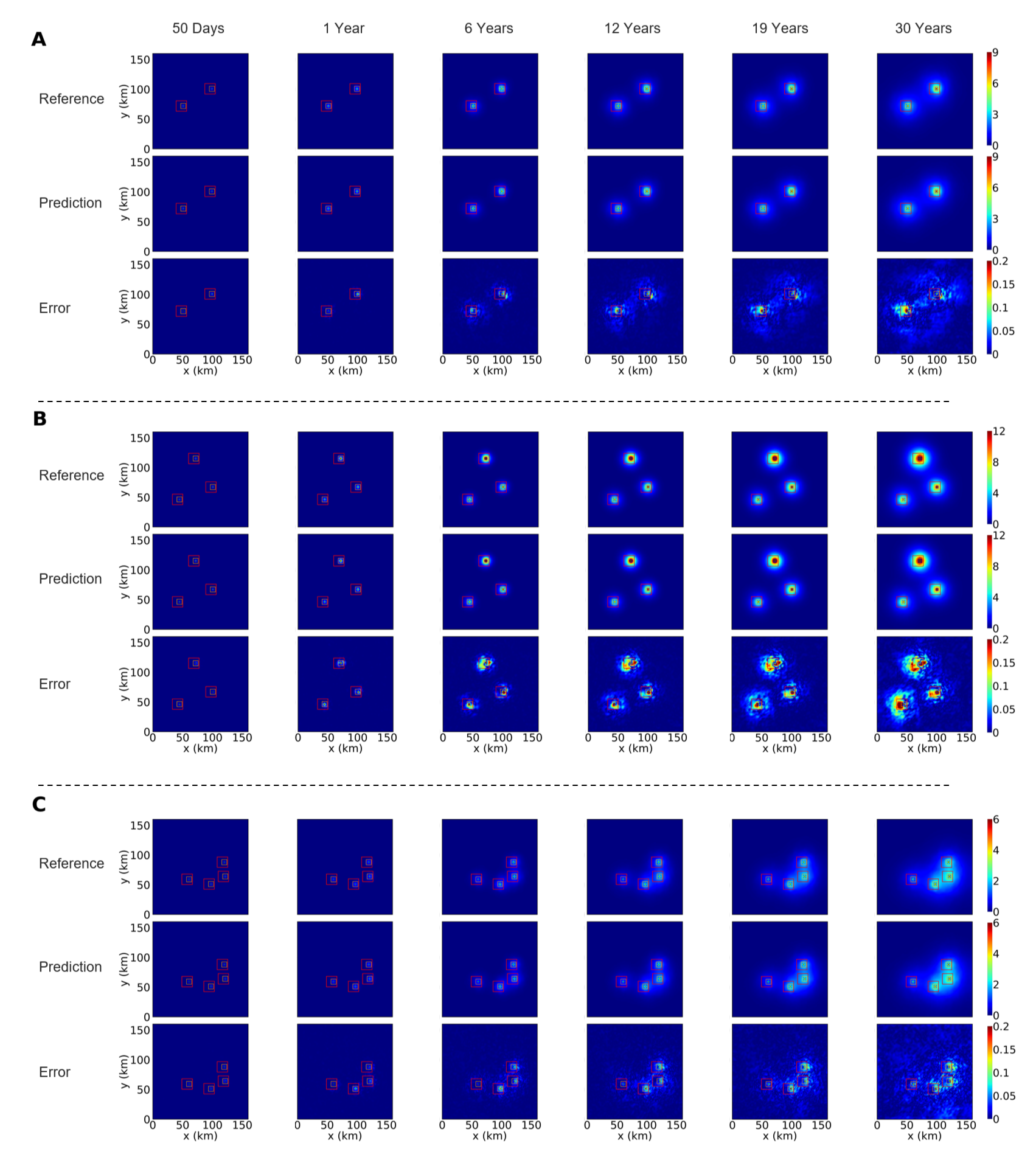
We show pressure buildup predictions and errors ($xy$-view at the top layer) of three randomly selected reservoirs with 2–4 wells at 6 different time snapshots, $T$ = {50d, 1.0y, 7.5y, 19.0y, 23.9y, and 30y} in Fig. 5. At early times where there is no significant pressure gradient, the error is the lowest. The error increases with time as the injection of CO₂ results in the buildup of pressure. For the pressure buildup of the first example (Fig. 5A), both cross-sectional $xy$-view at the top layer and $xz$-view around the injection point (level 1–4) are shown in Fig. 6A. By employing locally refined models, the errors are significantly reduced through predictions at refined resolutions.

For gas saturation network models, the accuracy of nested Fourier-DeepONet and nested FNO is also shown in Table 2. As mentioned in Section 3.4, we do not train the gas saturation model at the global level. As we were able to achieve better accuracy at the global level ($\delta^{P}_{\Omega_{0}}$) and level 1 ($\delta^{S}_{\Omega_{1}}$) for individual prediction (Table 6), the cumulative error arising from earlier levels resulted in lower accuracy with Fourier-DeepONets for both fine-tuned models and those without tuning. This highlights the importance of achieving robust accuracy at earlier levels when using a nested framework.

As shown in Fig. 6B, the CO₂ plume footprint is contained within the domain of level 1 even at 30 years of CO₂ injection. The error tends to be the largest at the boundary of the footprint in addition to the injection location.

To further investigate the generalizability of nested Fourier-DeepONet on unseen datasets, we conducted experiments to assess its performance under different extrapolation scenarios in terms of reservoir conditions (Sections 4.4.1 and 4.4.2), injection schemes (Section 4.4.3), and temporal coordinates (Section 4.4.4). For temporal extrapolation, we train models based on the first 21 time snapshots out of 24 while using all training samples.

References

- [1] Eclipse reservoir simulation software reference manual, 2014.
- [2] Blunt, M. J. Multiphase Flow in Permeable Media: A Pore-Scale Perspective. Cambridge University Press, Oct. 2016.
- [3] Bramble, J. H., Ewing, R. E., Pasciak, J. E., and Schatz, A. H. A preconditioning technique for the efficient solution of problems with local grid refinement. Computer Methods in Applied Mechanics and Engineering 67, 2 (Mar. 1988), 149–159.
- [4] Chen, T., and Chen, H. Universal approximation to nonlinear operators by neural networks with arbitrary activation functions and its application to dynamical systems. IEEE Transactions on Neural Networks 6, 4 (July 1995), 911–917.
- [5] Chen, Y., Lu, L., Karniadakis, G. E., and Dal Negro, L. Physics-informed neural networks for inverse problems in nano-optics and metamaterials. Optics Express 28, 8 (Apr. 2020), 11618.
- [6] Clark Di Leoni, P., Lu, L., Meneveau, C., Karniadakis, G. E., and Zaki, T. A. Neural operator prediction of linear instability waves in high-speed boundary layers. Journal of Computational Physics 474 (Feb. 2023), 111793.
- [7] Daneker, M., Cai, S., Qian, Y., Myzelev, E., Kumbhat, A., Li, H., and Lu, L. Transfer learning on physics-informed neural networks for tracking the hemodynamics in the evolving false lumen of dissected aorta. Nexus 1, 2 (June 2024), 100016.
- [8] Daneker, M., Zhang, Z., Karniadakis, G. E., and Lu, L. Systems Biology: Identifiability Analysis and Parameter Identification via Systems-Biology-Informed Neural Networks. Springer US, 2023, p. 87–105.
- [9] Deng, B., Shin, Y., Lu, L., Zhang, Z., and Karniadakis, G. E. Approximation rates of DeepONets for learning operators arising from advection–diffusion equations. Neural Networks 153 (Sept. 2022), 411–426.
- [10] Doughty, C. Investigation of CO2 plume behavior for a large-scale pilot test of geologic carbon storage in a saline formation. Transport in Porous Media 82, 1 (May 2009), 49–76.
- [11] Eigestad, G. T., Dahle, H. K., Hellevang, B., Riis, F., Johansen, W. T., and Øian, E. Geological modeling and simulation of CO2 injection in the johansen formation. Computational Geosciences 13, 4 (Aug. 2009), 435–450.
- [12] Faigle, B., Helmig, R., Aavatsmark, I., and Flemisch, B. Efficient multiphysics modelling with adaptive grid refinement using a mpfa method. Computational Geosciences 18, 5 (Mar. 2014), 625–636.
- [13] Fan, B., Qiao, E., Jiao, A., Gu, Z., Li, W., and Lu, L. Deep learning for solving and estimating dynamic macro-finance models. Computational Economics (Aug. 2024).
- [14] Hayford, J., Goldman-Wetzler, J., Wang, E., and Lu, L. Speeding up and reducing memory usage for scientific machine learning via mixed precision. Computer Methods in Applied Mechanics and Engineering 428 (Aug. 2024), 117093.
- [15] Jagtap, A. D., and Karniadakis, G. E. Extended physics-informed neural networks (XPINNs): A generalized space-time domain decomposition based deep learning framework for nonlinear partial differential equations. Communications in Computational Physics 28, 5 (2020).
- [16] Jiang, Z., Zhu, M., and Lu, L. Fourier-MIONet: Fourier-enhanced multiple-input neural operators for multiphase modeling of geological carbon sequestration. Reliability Engineering & System Safety 251 (2024), 110392.
- [17] Jiao, A., He, H., Ranade, R., Pathak, J., and Lu, L. One-shot learning for solution operators of partial differential equations. arXiv preprint arXiv:2104.05512 (2021).
- [18] Jin, P., Meng, S., and Lu, L. MIONet: Learning multiple-input operators via tensor product. SIAM Journal on Scientific Computing 44, 6 (Nov. 2022), A3490–A3514.
- [19] Kamashev, A., and Amanbek, Y. Reservoir simulation of CO2 storage using compositional flow model for geological formations in frio field and precaspian basin. Energies 14, 23 (Dec. 2021), 8023.
- [20] Karniadakis, G. E., Kevrekidis, I. G., Lu, L., Perdikaris, P., Wang, S., and Yang, L. Physics-informed machine learning. Nature Reviews Physics 3, 6 (May 2021), 422–440.
- [21] Khebzegga, O., Iranshahr, A., and Tchelepi, H. Continuous relative permeability model for compositional simulation. Transport in Porous Media 134, 1 (July 2020), 139–172.
- [22] Li, Z., Kovachki, N., Azizzadenesheli, K., Liu, B., Bhattacharya, K., Stuart, A., and Anandkumar, A. Fourier neural operator for parametric partial differential equations, 2020.
- [23] Lu, L., Jin, P., Pang, G., Zhang, Z., and Karniadakis, G. E. Learning nonlinear operators via DeepONet based on the universal approximation theorem of operators. Nature Machine Intelligence 3, 3 (Mar. 2021), 218–229.
- [24] Lu, L., Meng, X., Cai, S., Mao, Z., Goswami, S., Zhang, Z., and Karniadakis, G. E. A comprehensive and fair comparison of two neural operators (with practical extensions) based on FAIR data. Computer Methods in Applied Mechanics and Engineering 393 (Apr. 2022), 114778.
- [25] Lu, L., Meng, X., Mao, Z., and Karniadakis, G. E. Deepxde: A deep learning library for solving differential equations. SIAM Review 63, 1 (Jan. 2021), 208–228.
- [26] Lu, L., Pestourie, R., Johnson, S. G., and Romano, G. Multifidelity deep neural operators for efficient learning of partial differential equations with application to fast inverse design of nanoscale heat transport. Physical Review Research 4, 2 (June 2022).
- [27] Lu, L., Pestourie, R., Yao, W., Wang, Z., Verdugo, F., and Johnson, S. G. Physics-informed neural networks with hard constraints for inverse design. SIAM Journal on Scientific Computing 43, 6 (Jan. 2021), B1105–B1132.
- [28] Mao, S., Dong, R., Lu, L., Yi, K. M., Wang, S., and Perdikaris, P. PPDONet: Deep operator networks for fast prediction of steady-state solutions in disk–planet systems. The Astrophysical Journal Letters 950, 2 (June 2023), L12.
- [29] Mo, S., Zhu, Y., Zabaras, N., Shi, X., and Wu, J. Deep convolutional encoder‐decoder networks for uncertainty quantification of dynamic multiphase flow in heterogeneous media. Water Resources Research 55, 1 (Jan. 2019), 703–728.
- [30] Orr, F. M. Theory of gas injection processes. Tie-Line Publications, 2007.
- [31] Pruess, K., and García, J. Multiphase flow dynamics during CO2 disposal into saline aquifers. Environmental Geology 42, 2–3 (Mar. 2002), 282–295.
- [32] Remy, N., Boucher, A., and Wu, J. Applied Geostatistics with SGeMS: A User’s Guide. Cambridge University Press, Jan. 2009.
- [33] Tang, M., Liu, Y., and Durlofsky, L. J. A deep-learning-based surrogate model for data assimilation in dynamic subsurface flow problems. Journal of Computational Physics 413 (July 2020), 109456.
- [34] Wen, G., and Benson, S. M. CO2 plume migration and dissolution in layered reservoirs. International Journal of Greenhouse Gas Control 87 (Aug. 2019), 66–79.
- [35] Wen, G., Hay, C., and Benson, S. M. CCSNet: a deep learning modeling suite for CO2 storage. Advances in Water Resources 155 (2021), 104009.
- [36] Wen, G., Li, Z., Long, Q., Azizzadenesheli, K., Anandkumar, A., and Benson, S. M. Real-time high-resolution CO2 geological storage prediction using nested fourier neural operators. Energy & Environmental Science 16, 4 (2023), 1732–1741.
- [37] Wen, G., Tang, M., and Benson, S. M. Towards a predictor for CO2 plume migration using deep neural networks. International Journal of Greenhouse Gas Control 105 (Feb. 2021), 103223.
- [38] Wu, C., Zhu, M., Tan, Q., Kartha, Y., and Lu, L. A comprehensive study of non-adaptive and residual-based adaptive sampling for physics-informed neural networks. Computer Methods in Applied Mechanics and Engineering 403 (Jan. 2023), 115671.
- [39] Wu, W., Daneker, M., Jolley, M. A., Turner, K. T., and Lu, L. Effective data sampling strategies and boundary condition constraints of physics-informed neural networks for identifying material properties in solid mechanics. Applied Mathematics and Mechanics 44, 7 (July 2023), 1039–1068.
- [40] Yazdani, A., Lu, L., Raissi, M., and Karniadakis, G. E. Systems biology informed deep learning for inferring parameters and hidden dynamics. PLOS Computational Biology 16, 11 (Nov. 2020), e1007575.
- [41] Yu, J., Lu, L., Meng, X., and Karniadakis, G. E. Gradient-enhanced physics-informed neural networks for forward and inverse pde problems. Computer Methods in Applied Mechanics and Engineering 393 (Apr. 2022), 114823.
- [42] Zhang, Z., Moya, C., Lu, L., Lin, G., and Schaeffer, H. D2NO: Efficient handling of heterogeneous input function spaces with distributed deep neural operators. Computer Methods in Applied Mechanics and Engineering 428 (Aug. 2024), 117084.
- [43] Zhu, M., Feng, S., Lin, Y., and Lu, L. Fourier-DeepONet: Fourier-enhanced deep operator networks for full waveform inversion with improved accuracy, generalizability, and robustness. Computer Methods in Applied Mechanics and Engineering 416 (2023), 116300.
- [44] Zhu, M., Zhang, H., Jiao, A., Karniadakis, G. E., and Lu, L. Reliable extrapolation of deep neural operators informed by physics or sparse observations. Computer Methods in Applied Mechanics and Engineering 412 (2023), 116064.
- [45] Zhu, Y., and Zabaras, N. Bayesian deep convolutional encoder–decoder networks for surrogate modeling and uncertainty quantification. Journal of Computational Physics 366 (Aug. 2018), 415–447.