Effective Elastic Properties of Multilayer Graphene

Multilayered two-dimensional (2D) materials have highly anisotropic elastic behaviors due to their unique atomic structure [1, 2, 3]. Single layer is formed by covalent bonds while neighboring layers are bound by van der Waals (vdW) interaction. The vdW interaction, though it is weaker in materials compared with the ionic, covalent and metallic bonds [4], is essential for constructing various multilayered 2D materials [5, 6]. In graphite, the strong $sp^{2}$ covalent bond makes a hexagonal lattice while layers glues together by the weak vdW attraction [7].

Owing to anisotropic natures in their structures, many physical properties of layered materials such as electrical, thermal and optical ones change their characteristics from their 2D limit to three-dimensional (3D) bulk ones depending on the number of layers ($N_{\text{lay}}$) [8, 9, 10]. Their mechanical properties may also alter accordingly. Based on currently available studies [11, 12, 13, 14, 15, 16, 17, 18, 19, 20, 21, 22], the dimensional dependence of mechanical properties of graphene, especially Young’s modulus ($E$), is not thoroughly investigated. When the thickness of multilayer graphene samples increases, all three possibilities for variation of $E$ – increase, decrease or remain unchanged – have been reported [11, 12, 13, 14, 15, 16, 17, 18, 19, 20, 21, 22]. Questions such as whether there is any dimensional crossover or transition for mechanical properties, and if there is, what is the critical $N_{\text{lay}}$ and which physical parameter dominates, are important and fundamental, but have not been answered conclusively so far.

In this Letter, we explore the elastic behaviors of graphene such as variations of its $E$ and Grüneisen parameter ($\gamma$) with increasing its thickness from one to twenty one layers through in-situ bulge tests together with simultaneous spectroscopic measurements. We also perform extensive first-principles calculations based on density functional theory (DFT) as well as mechanical model calculations to consider realistic situations beyond simple periodic unitcell geometries for DFT calculations. Our main finding is a sharp dichotomy between measurements and computational results such that calculated $E$ [23] and $\gamma$ are independent of $N_{\text{lay}}$ while our measured ones substantially decrease with increasing thickness. We found that the origin of such a discrepancy is inevitable experimental overestimation of strains owing to their intrinsic difference between inter- and intra-layer mechanical couplings. We believe that our finding of experimental circumscription in measuring mechanical properties of multilayer graphene would also be unavoidable for other layered materials. Through careful analysis, we propose a new mechanical modulus of $E/\gamma^{3/2}$ to characterize intrinsic mechanical properties of multilayered vdW materials free from uncontrollable interlayer slidings.

We prepare graphene samples with various thickess ranging from single to twenty one layers. Figure 1(a) shows optical images of some graphene samples. To determine $N_{\text{lay}}$ precisely, we mainly use optical transmittance [10] and Raman spectroscopy shown in Fig. 1 (b) and (d), respectively [24, 25]. Up to seven layers, Raman spectroscopy determines the number of layers. Optical transmittance data is fit to $N_{\text{lay}}$ and extrapolated over seven layers to determine $N_{\text{lay}}$. TEM [26] measurements were also carried out to cross check the thickness.

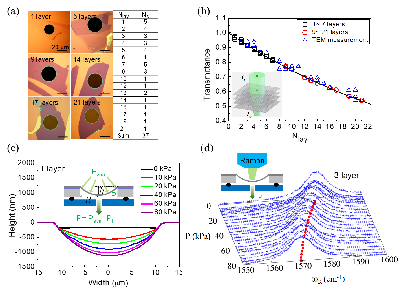
To measure $E$ and $\gamma$, in-situ bulge tests are performed along with atomic force microscopy (AFM) as shown in Fig. 1 (c) and Raman spectroscopy in Fig. 1(d). Stress is applied to graphene using pressure difference of $P$ between the atmospheric ($P_{\rm atm}$) and the vacuum chamber pressure ($P_{\rm i}$). In order to avoid delamination of graphene from the substrate, we set $P_{\rm i}$ to be smaller than $P_{\rm atm}$. The bulge height of $h$ is measured by a non-contact mode of AFM as shown in Fig. 1(c). Using $P$ and $h$, stress and strain of deformed graphene samples are obtained from the analytical formula for a typical bulge test shown in Eq. (1). To measure $\gamma$, the Raman shift as a function of equibiaxial strain is obtained from the in-situ Raman-bulge test as shown in Fig. 1(d). The positions of Raman $G$ and $2D$ bands are obtained from Lorentzian fitting for each strain. Here, only the Grüneisen parameter for the $G$ band is used to simplify our analysis (see SI for experimental details).

In a bulge test, with the assumption of perfect clamping on the edge, the values of biaxial strain and stress at the center of the bulge are approximately $\epsilon={2h^{2}/3R^{2}}$ and $\sigma={PR^{2}/4ht}$ [27] so that Young’s modulus can be written as

where $P$, $h$, $R$, $t$ and $\nu$ are applied pressure, the bulge height, radius of the hole, the thickness and the Poisson’s ratio of the sample in Fig. 2(a). With dimensionless expressions, $\bar{q}\equiv\frac{PR}{Et}$, $\bar{\sigma}\equiv\frac{\sigma}{E}$, $\bar{h}\equiv\frac{h}{R}$ and $k=\frac{8}{3(1-\nu)}$, Eq. (1) can be rewritten as

where

In our experiments, the bulge height is measured as a function of applied pressure for various samples with varying $N_{\rm lay}$. The diameter of the hole for different samples ranges from 20 to 30 $\mu$m. We calculate the values of Young’s modulus of multilayer graphene depending on $N_{\rm lay}$ using Eq. (1) with inputs from our experimental data and results are plotted in Fig. 3(d). It shows that the experimental Young’s modulus decreases substantially as $N_{\rm lay}$ increases. On the other hand, a previous DFT report shows that the Young’s modulus of multilayer graphene is barely dependent on $N_{\rm lay}$ (plotted in Fig. 3(d)) [23]. In this work, we show that the experimental deviation from the DFT result is attributed to the imperfect clamping of the graphene to the substrate as well as the interlayer sliding between graphene layers [7].

With interlayer sliding, interlayer shear strength ($\tau$) or the maximum value of interlayer shear stress is built against the direction of sliding. It is the force that gives a static friction. We use dimensionless interlayer shear strength, $\bar{\tau}\equiv\tau R/Et$. Wang et. al. estimated the values of $\tau$ between graphene and SiO₂ substrate and between graphene and graphene using bulge tests [7]. Hereafter, the former is denoted by $\tau_{\rm gs}$ and the latter $\tau_{\rm gg}$. They found that, when the suspended graphene within a hole of the substrate is pressurized, shear stress is built due to interlayer sliding across the supported region outside the hole which is to be balanced againt the intralayer stress within the suspended region. Their approch was successful for single and bilayer graphene. The method, however, cannot be applied for more than two layers.

The key to understand the bulge test in the presence of the interlayer sliding lies on proper estimation on a distance how far the sample on the rim around the hole is pulled inward. This additional pulling would give an additional contribution to the bulge height so that the sample would look softer than the case without it. Let us first consider a single layer case with this effect. The equation of equilibrium of graphene in the supported region outside of the hole can be written as

where dimensionless radial distance is defined by $\rho\equiv r/R$. The stress for the region with $\rho<1$ obtained by Eq. (3) is most valid near the center of the hole. As $\rho\rightarrow 1$ from the inside, azimuthal component of stress becomes very small – no stretch along the circumferential direction – so that the radial component of stress should become roughly double the value of Eq. (3). With conditions for isotropy and continuity of $\bar{\sigma}_{r}$ at $r=R$, the solutions are

where $A=\frac{1}{2}\left({1-\nu^{2}}\right)\bar{\tau}\rho_{\rm max}$ and $B=-\frac{1}{6}\left({1-\nu^{2}}\right)\bar{\tau}\rho_{\rm max}^{3}.$ Here, $\rho_{\rm max}$ is the solution of a cubic equation of $x$, $\frac{{1-\nu}}{6}\left(x-1\right)^{3}+\frac{{1-\nu}}{2}\left(x-1\right)^{2}+(x-1)={\zeta}{\left[{3(1-\nu)}\right]^{-\frac{1}{3}}}$ where $\zeta\equiv\bar{q}^{2/3}/\bar{\tau}$. Here, $\rho_{\rm max}$ represents another boundary condition such that $\sigma_{r}$ and $\sigma_{\theta}$ simultaneously vanishes at $\rho=\rho_{\rm max}$. Strains can be obtained using $\epsilon_{r}=\bar{\sigma}_{r}-\nu\bar{\sigma}_{\theta}$ and $\epsilon_{\theta}=\bar{\sigma}_{\theta}-\nu\bar{\sigma}_{r}$ (see SI for detailed derivation).

Now, the radial displacement is $\bar{u}_{r}=\rho\epsilon_{\theta}$ in an isotropic system, whose value at $\rho=1$ represents the amount of pulling-in of graphene at the rim of the hole; $\bar{u}_{r}(\rho=1)=-\frac{(1-\nu^{2})}{6}\bar{\tau}[(\rho_{\text{max}}-1)^{3}+3(\rho_{\text{max}}-1)^{2}].$ As depicted schematically in Fig. 2(b), this pulling-in provides additional contribution to the bulge height, $\bar{h}_{1}=-\bar{u}_{r}(\rho=1)$, so that the total bulge height becomes $\bar{h}=\bar{h}_{0}+\bar{h}_{1}$, where $\bar{h}_{0}$ is from Eq. (2).

In case of perfect clamping, $\bar{\tau}\rightarrow\infty$ and $\zeta\rightarrow 0$ so that $\rho_{\rm max}\rightarrow 1$ and $\bar{h}_{1}$ becomes zero. Then, the relation between $\bar{q}$ and $\bar{h}^{3}$ becomes the same as Eq. (2). With graphene-substrate sliding allowed, i.e., $\bar{h}_{1}\neq 0$, the coefficient $k$ in Eq. (2) becomes dependent on $\bar{\tau}$ and $\zeta$,

where $f(x)\equiv\left(x-1\right)^{3}+3\left(x-1\right)^{2}.$ For two limiting cases, $\zeta\ll 1$ and $\zeta\gg 1$ with $\nu=0.144$ [23], $k_{\bar{\tau}}(\zeta)$ can be approximated as

and

respectively. Recalling that $\zeta=\frac{\bar{q}^{2/3}}{\bar{\tau}}$, $\bar{q}=\frac{PR}{Et}$ and $\bar{\tau}=\frac{\tau R}{Et}$, Eqs. (8) and (9) show that $k_{\bar{\tau}}(\zeta)$ begins to decrease from the perfect clamping case if $P\sim\tau$ and approaches to zero if $P>Et/R$. These two criteria determine the overall shape of the $k$ vs. $P$ graph. For our experiments, the second criteria becomes $Et/R\sim 35$ MPa, with $R\sim 10~{}\mu$m, $t=3.35$ Å and $E=1075$ GPa. Our experimental condition which is up to about several tens kPa is not in such an extreme regime but near the first criteria.

For each given pressure, we calculate $\bar{h}$ and corresponding $k$ using Eq. (7). Figure 3(a) shows $k$ as a function of $P$ for two different values of $\tau$ such as $\tau_{\rm gg}=40$ kPa and $\tau_{\rm gs}=1640$ kPa [7]. The value of $k$ begins to decrease at different pressures corresponding to each $\tau$ value, while $k$ supresses to zero over the same pressure, $Et/R$. The hatched area is our experimental pressure range. Because of the interlayer sliding effect considered in Eq. (7), $\bar{q}$ is not simply proportional to $\bar{h}^{3}$. Figure 3(b) shows the amount of deviation from the linear correlation (dotted line) upto the hatched area in Fig. 3(a).

Let us consider multilayer cases for which shear stress should be distributed properly across the layers with the maximal value limited by $\tau$. Figure 2(c) shows the configuration of the distribution of interlayer shear stresses; the difference between neighboring shear stresses should be balanced with the intralayer stress of the strained graphene in the suspended region. In order for all the upper layers except the bottom layer move harmonically together, differences between stresses on neighboring layers should be the same so that the interlayer shear stress must increase monotonically from the top to lower layers. For example, in the case of five-layer graphene on a substrate, the distribution of interlayer shear stress should be like Fig. 2(c). All the layers except the bottom layer experience the same net radial stress of $\tau_{\rm gg}/4$. It allows each layer’s $\rho_{\rm max}$ and corresponding $\bar{h}$ to be all simultaneously the same if the total pressure is equally distributed except the bottom layer. Bottom layer experiences a net stress of $\tau_{\rm gs}-\tau_{\rm gg}$. Total pressure of $P$ is distributed across the layers such that $P=(N_{\rm lay}-1)P_{\rm u}+P_{\rm b}$. Here, the ratio between $P_{\rm u}$ and $P_{\rm b}$ is determined to make the bulge heights of the layers to have the same value of $h$. The bulge height for the $i$-th layer for a given pressure of $P_{i}$ is calculated using the same procedure as in the single layer case and the subscripts ‘u’ and ‘b’ represent the upper and bottom layers, respectively.

We first calculate $h$ based on the theoretical model discussed so far in case of constant Young’s modulus of graphene regardless of $N_{\rm lay}$ as was obtained from DFT results [23]. Figure 3(c) compares calculated $h$ with varying $P$ for trilayer graphene with experimental results. The inset shows corresponding $\sigma$ vs. $\epsilon$. We note that a constant offset for the measured height from the model calculation do not affect their ratio or the computed Young’s modulus seriously. Let us call this Young’s modulus obtained with a simple ratio of $(1-\nu){\frac{\sigma}{\epsilon}}$ as ‘apparent Young’s modulus’ or $E_{\text{ap}}$. Solid squares in Fig. 3(d) are the theoretical estimation of $E_{\text{ap}}$ using our sample geometries, while the crosses are directly from the experiments. One can see that the theoretical $E_{\text{ap}}$ decreases as $N_{\text{lay}}$ increases and saturates around $N_{\text{lay}}\simeq 10$ and that our model calculations and measurements match pretty well. So, we may consider ten layers as a critical thickness for mechanical crossover from 2D to 3D characteristics. However, for samples thicker than ten layers, the both deviate each other significantly.

Before discussing the serious discrepancies for cases with $N_{\text{lay}}>10$, it is worthwhile to compare $E_{\text{ap}}$ for multilayers with one for single layer. As shown in Eq. (2), $E_{\text{ap}}$ is proportional to $k$, reflecting effects from substrates. So, $E_{\text{ap}}$ decreases to $1034$ GPa from its intrinsic $1075$ GPa for graphene on SiO₂ substrate and to $827$ GPa for graphene on graphene. The overall $E_{\text{ap}}$ is areal average so that, as $N_{\rm lay}$ increases, the value approaches to that for graphene on graphene. In Fig. 3(d), $E_{\text{ap}}$ for the case with $\tau=\tau_{\rm gs}$ and for the case with $\tau=\tau_{\rm gg}$ are drawn with dashed lines. As discussed, $E_{\text{ap}}$ begins with the value for $\tau=\tau_{\rm gs}$ and approaches to one for $\tau=\tau_{\rm gg}$ as $N_{\rm lay}$ increases.

As shown in Fig. 3(d), our estimated $E$ for cases of $N_{\text{lay}}>10$ deviates from the experimental results, for which we suspect two major sources. One is a formation of wrinkles [20, 22] and the other is delamination of layers. Because of $\bar{u}_{r}=\rho\epsilon_{\theta}$, isotropic pull of graphene toward the center of the hole causes azimuthal compression, possibly forming wrinkles along the radial direction especially near the edge of the hole where pressurized graphene is structurally unstable due to bending and the instability increases with thickness. Such wrinkles practically reduce intrinsic $E$ under compression along the circumferential direction so that the shape of Fig. 3(a) changes by shifting one of the pressure criteria, $Et/R$, toward lower $P$. This, together with the reduction of $\tau_{\rm gs}$ due to delamination, further reduces $k$ within our pressure range as well as $E_{\rm ap}$.

To further consider the wrinkle and delamination effects, we first estimate $N_{\text{lay}}$-dependent $\gamma$ using DFT method [28]. Detailed computational parameters are in Supplementary Information. For each number of layers, phonon frequencies of $\omega_{G}$ corresponding to the Raman G peak are calculated for isotropic strains of $\epsilon$ increasing from $-0.02$ to $0.02$. Using $\gamma=-{\partial\ln\omega_{G}}/{\partial\epsilon}$ [29, 30] (an example for trilayer is shown in Fig. 4(a)), we obtain $\gamma$ for doubly degenerate $2N_{\rm lay}$ modes [31, 32, 33] of multilayer graphene with $N_{\text{lay}}$ [Fig. 4(b)]. We note that the splitting is about one percent of the average values. For $N_{\text{lay}}=1$, our DFT result agrees with a previous report [33]. In Fig. 4(c), the measured Grüneisen parameters from Raman spectrum are shown to decrease as the number of layers increases in contrast to the constancy of averaged $\gamma$ from our DFT calculation. We find that this discrepancy can also be attributed to the strain overestimation like $E_{\text{ap}}$.

Let $\tilde{\epsilon}$ and $\tilde{\sigma}$ be the intrinsic or ideal values of strain and stress averaged over the layers. The averaged strain $\tilde{\epsilon}$ should be determined by $h_{0}$ instead of $h$ such that $\tilde{\epsilon}=(2/3)(h_{0}/R)^{2}$, although $h_{0}$ cannot be extracted from experiment directly. Since the intrinsic Young’s modulus of $\tilde{E}=(1-\nu)(3R^{4}/8t)(P/h_{0}^{3})=1075$ GPa is independent of $N_{\text{lay}}$ [23], $\tilde{\epsilon}$ can be estimated from $\epsilon$ using the ratio of measured $E=(1-\nu)(3R^{4}/8t)(P/h^{3})$ such that

This formula shows a quantitative scale for the overestimated $\epsilon$ using the measured (hence, underestimated) $E$. The same procedure for intrinsic Grüneisen parameter of $\tilde{\gamma}$ that is also independent of $N_{\text{lay}}$ results in

Here, we note that the measured $\gamma$ is underestimated by the same factor for underestimated strain in Eq. (10). A prefactor in Eq. (11) can be used to rescale our constant Grüneisen parameter obtained from DFT calculations as a function of $N_{\text{lay}}$ and then resulting $\gamma$’s show a good agreement with our measurements as shown in Fig. 4(d).

Considering consequences from incomplete strain transfer or delamination behaviors discussed so far, we propose a new mechanical constant coined as elastic Grüneisen modulus, $E_{\gamma}\equiv E/\gamma^{3/2}$, which is robust against the inevitable experimental underestimation of strain in vdW materials. In Fig. 4(d), $E_{\gamma}$’s for our experiment are nearly independent of $N_{\text{lay}}$ and match well with the constant DFT result, thus reflecting intrinsic mechanical properties of layered materials.

In conclusion, we have measured critical elastic properties of multilayer graphene such as Young’s modulus and Grüneisen parameter and analyzed them carefully by including shear sliding between layers. Unlike constant intrinsic values for those parameters from ab initio calculations, our measured values show strong thickness dependent characteristics, of which origins we attributed to the unavoidable layer slidings. We further propose a new material constant of elastic Grüneisen modulus that is experimentally robust against interlayer shear effects. Considering that similar mechanical properties are shared by almost all vdW materials [23, 34, 35, 36, 37] , we believe that our new mechanical parameter will be of importance in extracting intrinsic mechanical properties from experiments.