Effective boundary conditions for dynamic contact angle hysteresis on chemically inhomogeneous surfaces
Abstract
Recent experiments (Guan et al., 2016a, b) showed many interesting phenomena on dynamic contact angle hysteresis while there is still a lack of complete theoretical interpretation. In this work, we study the time averaging of the apparent advancing and receding contact angles on surfaces with periodic chemical patterns. We first derive a Cox-type boundary condition for the apparent dynamic contact angle on homogeneous surfaces using Onsager variational principle. Based on this condition, we propose a reduced model for some typical moving contact line problems on chemically inhomogeneous surfaces in two dimensions. Multiscale expansion and averaging techniques are employed to approximate the model for asymptotically small chemical patterns. We obtain a quantitative formula for the averaged dynamic contact angles. It gives explicitly how the advancing and receding contact angles depend on the velocity and the chemical inhomogeneity of the substrate. The formula is a coarse-graining version of the Cox-type boundary condition on inhomogeneous surfaces. Numerical simulations are presented to validate the analytical results. The numerical results also show that the formula characterizes very well the complicated behaviour of dynamic contact angle hysteresis observed in the experiments.
1 Introduction
Wetting is a fundamental process in nature and our daily life (De Gennes (1985); Bonn et al. (2009)). It is of critical importance in many industrial applications, e.g., coating, printing, chemical engineering, oil industry, etc. The wetting property is mainly characterized by the contact angle between the liquid-vapor interface and the solid surface. When a liquid drop is in equilibrium on a homogeneous smooth surface, the contact angle is described by the famous Young’s equation (Young, 1805). The equilibrium contact angle, also named Young’s angle, depends on the surface tensions and reflects the material properties of the substrate. However, the real surface is usually neither homogeneous nor smooth and the chemical and geometric inhomogeneity may affect the wetting property dramatically. This makes the wetting phenomena very complicated in real applications, especially for dynamic problems.
For a liquid drop on an inhomogeneous surface, the apparent contact angle is usually different from the microscopic contact angle near the contact line even in equilibrium state. The equilibrium state of a droplet is determined by minimizing the total free energy of the system. When a global minimum is obtained, the apparent contact angle of a liquid can be described either by the Wenzel equation (Wenzel (1936)) or by the Cassie-Baxter equation (Cassie & Baxter (1944)). In reality, there exist many local minimizers that can not be described by the two equations (c.f. Gao & McCarthy (2007); Marmur & Bittoun (2009)). One can observe many equilibrium contact angles in experiments. The largest contact angle is called the advancing contact angle and the smallest one is the receding contact angle. The difference betweene the advancing angle and the receding one is usually referred to the (static) contact angle hyteresis (CAH).
The static contact angle hysteresis has been studied a lot in the literature (see e.g. Johnson Jr. & Dettre (1964); Neumann & Good (1972); Cox (1983); Joanny & De Gennes (1984); Schwartz & Garoff (1985); Extrand (2002); Priest et al. (2007); Whyman et al. (2008) among many others). For a two dimensional problem, the contact line is reduced to a point. When the surface is chemically composed of two or more materials with different Young’s angles, it is found that the advancing contact angle is equal to the largest Young’s angle in the system and the receding contact angle equals the smallest Young’s angle(see Johnson Jr. & Dettre (1964); Xu & Wang (2011)). For a three dimensional problem, the situation becomes more complicated. The contact angle hysteresis due to a single defect on a homogeneous solid surface was analysed in Joanny & De Gennes (1984). The analysis can be generalized to surfaces with dilute defects. Recently, some modified Wenzel and Cassie equations are proposed to characterize quantitatively the local equilibrium contact angle and the contact angle hysteresis in Choi et al. (2009); Raj et al. (2012); Xu & Wang (2013); Xu (2016). By these equations, the apparent contact angle can be computed once the position of the contact line is given. However, since the actual position of a contact line usually depends on the dynamic process (see Iliev et al. (2018)), we need study the dynamic wetting problem for real applications.
Dynamic wetting is much more challenging than the static case due to the motion of the contact line, which is still an unsolved problem in fluid dynamics (see Pismen (2002); Blake (2006); Snoeijer & Andreotti (2013); Sui et al. (2014)). The standard no-slip boundary condition may lead to a non-physical non-integrable stress in the vicinity of the contact line (Huh & Scriven, 1971; Dussan, 1979). To cure this paradox, many models were developed. A natural way is to explicitly adopt the Navier slip boundary condition instead of the no-slip condition (Huh & Scriven, 1971; Zhou & Sheng, 1990; Haley & Miksis, 1991; Spelt, 2005; Ren & E, 2007) or implicitly impose the slip effect by numerical methods (Renardy et al., 2001; Marmottant & Villermaux, 2004). Some other approaches include: to assume a precursor thin film and a disjoint pressure (Schwartz & Eley, 1998; Pismen & Pomeau, 2000; Eggers, 2005); to introduce a new thermodynamics for surfaces (Shikhmurzaev, 1993); to treat the moving contact line as a thermally activated process (Blake, 2006; Blake & De Coninck, 2011; Seveno et al., 2009), to use a diffuse interface model for moving contact lines (Seppecher, 1996; Gurtin et al., 1996; Jacqmin, 2000; Qian et al., 2003; Yue & Feng, 2011), etc. Most of these models can be regarded as a microscopic model for moving contact lines, due to the existence of very small parameters, e.g. the slip length and the diffuse interface thickness, etc. It is very expensive to use them in quantitative numerical simulations for dynamic wetting problems, unless the characteristic size of the problem is very small (Gao & Wang (2012); Sui et al. (2014)).
To simulate the macroscopic wetting problem efficiently, various effective models have been proposed. One important model is the so-called Cox’s model developed in Cox (1986) for viscous flows. The relation between the (macroscopic) apparent contact angle and the contact line velocity (characterized by the capillary number) is derived by matched expansions and asymptotic analysis. The model was further validated and developed in Sui & Spelt (2013b); Sibley et al. (2015), and generalized in Ren et al. (2015); Zhang & Ren (2019) for distinguished limits in different time regimes. In real simulations, one can use the macroscopic model directly and there is no need to resolve the microscopic slip region in the vicinity of the contact line. This improves significantly the efficiency of the numerical methods and make it possible to quantitatively simulate some macroscopic moving contact line problems (Sui & Spelt (2013a)).
To study the dynamic contact angle hysteresis, one needs to consider the moving contact line problems on (either geometrically or chemically) inhomogeneous surfaces. The problem has been studied theoretically in Raphael & de Gennes (1989) and Joanny & Robbins (1990) for the single defect case. For the moving contact line problems with chemically patterned substrates, theoretical study is more difficult. Direct numerical simulations in two dimensions have been done in Wang et al. (2008) and Ren & E (2011). In these simulations, the authors adopted some standard microscopic moving contact line models where the inhomogeneity of the substrates are described explicitly in the boundary conditions. The stick-slip behaviour of the contact lines was observed. The contact angle hysteresis was also observed when the period of the chemical pattern is small. The main challenge in direct simulations is that the computational complexity is very large in order to resolve the microscopic inhomogeneity. Besides the direct simulations, more studies were done by using phenomenological contact angle hysteresis models(Dupont & Legendre (2010); Zhang & Yue (2020); Yue (2020)), where the advancing and receding contact angles were given a priori and the contact line can not move unless the dynamic contact angle was beyond the interval bounded by the two angles. The advancing and receding contact angles in these models are effective parameters. In general, it is not clear how the parameters are related to the chemical inhomogeneity of the substrates.
More recently, some experimental results on the dynamic contact angle hysteresis have been presented in Guan et al. (2016a, b). The authors showed many interesting properties on the dynamic advancing and receding contact angles. Both the advancing and receding contact angles can change with the increase of the contact line velocity. The dependence of the contact angles on the velocity is quite complicated. Sometimes it seems symmetric while it can be very asymmetric in other cases. The asymmetric dependence is partially understood from the distributions of the chemical patterns(see Xu et al. (2019); Xu & Wang (2020)). But there is still a lack of complete understanding of all the experimental results.
The motivation of the work is two folds. Firstly, we would like to develop an averaged Cox-type boundary condition for moving contact lines on inhomogeneous surfaces. The boundary condition characterizes quantitatively how the macroscopic advancing and receding angles depend on the microscopic inhomogeneity of the substrates. With this condition, a macroscopic model may be developed for dynamic contact angle hysteresis. Secondly, we would also like to have more theoretical understandings on the complicated phenomena of dynamic contact angle hysteresis in recent experiments in Guan et al. (2016a, b).
For these purposes, we conduct our study in two steps. First, we derive a simplified Cox-type boundary condition for moving contact lines on general surfaces. The main tool here is to use the Onsager variational principle as an approximation tool. Recent studies showed that it is very useful for approximately modelling many complicated problems in viscous fluids and in soft matter( c.f. Doi (2015); Xu et al. (2016); Di et al. (2016); Man & Doi (2016); Zhou & Doi (2018); Guo et al. (2019); Doi et al. (2019); Xu & Wang (2020)). In this paper, we show that the principle can be used to derive a full sharp-interface model and a new simplified Cox-type boundary condition for moving contact lines. The boundary condition is a first order approximation for the original Cox’s condition. With the condition, we can construct a reduced model for some interesting moving contact line problems, including the one for the experiments in Guan et al. (2016a, b). Second, we do asymptotic analysis for the reduced model on chemically inhomogeneous substrates. By multiscale expansions, we derive an averaged dynamics for the contact angle and the contact point. This leads to an explicit formula for the averaged (in time) macroscopic dynamic contact angle on chemically inhomogeneous surfaces. The formula is a coarse-graining boundary condition for dynamic contact angle hysteresis. Our analysis is validated by numerical experiments. Furthermore, numerical examples show that the reduced model and the new boundary conditions can be used to understand the complicated behaviours of the apparent contact angles observed in the experiments in Guan et al. (2016a, b). All the main phenomena can be captured by the reduced model and described by the averaged formula.
Although the averaging analysis is conducted for a reduced model in the paper, the averaged boundary condition for dynamic contact angle hysteresis is quite general, since it does not depends on the specific setup of the problem at all. The condition is a form of harmonic average of the simplified Cox-type boundary condition. The main result can also be generalized to the case where the original Cox’s boundary condition applies. We expect that the formulae for the averaged macroscopic dynamic contact angles can be used as an effective boundary condition for the two-phase Navier-Stokes equation for moving contact lines on inhomogeneous surfaces.
Although the analysis in this paper is restricted to two-dimensional problems, the main results can be used to understand some three dimensional contact angle hysteresis problems, e.g. on an inhomogeneous surface with dilute defects. Nevertheless, quantitative descriptions for general three dimensional problems are still challenging and will be left for future study.
The structure of the paper is as follows. In Section 2, we introduce the derivations for a continuum model and a Cox-type boundary condition for moving contact lines in a variational approach. A reduced model is presented for some specific problems. In Section 3, we do asymptotic analysis for the reduced model to derive the averaged dynamics on chemically inhomogeneous surfaces. Explicit formulae for the apparent dynamic contact angles are derived. In Section 4, we validate the asymptotic analysis numerically and do comparisons with experiments. Finally, in Section 5 we give some concluding remarks, especially discussions on the generalization to three-dimensional moving contact line problems.
2 Variational derivation for moving contact line models
In this section, we will derive two types of models for moving contact lines by a variational approach. The first one is a full continuum model consisting of a partial differential equation system and the boundary conditions on the microscopic contact angle. The second one is a Cox-type boundary condition, which describes the dynamics of the apparent contact angle. The Cox-type boundary condition is employed to further reduce the model for two typical problems with moving contact lines. The reduced model acts as a model problem to study the dynamic contact angle hysteresis in the following sections.
2.1 Derivation for a continuum model for moving contact lines

Consider a region near the contact line as in Figure 1. For simplicity, we suppose is a two-dimensional domain. The boundary of is composed of two parts, the lower solid boundary and the outer boundary . On , there exists a moving contact line, which is an intersection point between the solid boundary and the two-phase flow interface . Then represents an open system near the contact point. In the following, we will derive a sharp interface continuum model for moving contact lines. We adopt the Onsager principle to derive the model. The method has been used to develop the generalized Navier slip boundary condition for a diffuse interface model in Qian et al. (2006). In the derivation, we ignore the gravitational force and the inertial effect, which can be added simply if needed.
To use the Onsager principle, we first compute the rate of change of the total energy in the system. The total free energy consists of three interface energies,
| (2.1) |
where and are respectively the parts of solid boundary in contact with the fluid and fluid , and are corresponding surface tensions, and is the surface tension of the two-phase flow interface. Direct calculations give
| (2.2) |
Here is the dynamic contact angle with respect to the fluid , is Young’s angle, is the velocity of the contact line, is the normal velocity, and is the curvature of the interface. In the derivation, we have also used the Young’s equation .
The energy dissipation function, which is defined as half of the total energy dissipation rate in the system, can be written as
| (2.3) |
where and are the regions in occupied by fluid A and fluid B, respectively, is the corresponding velocity field, is the slip velocity on the solid boundary, and are viscosity parameters, and are phenomenological slip coefficients, and is the friction coefficient of the contact line. The normal velocity on the solid boundary is zero.
Since the system is an open system, we need also consider the work to the outer fluids at the boundary . It is given by
| (2.4) |
where and are the respective open boundary in contact with fluid A and fluid B.
With the above definitions, the Onsager principle states that (Doi, 2013) the dynamical equation of the system is given by minimizing the Onsager-Machlup action defined as follows
| (2.5) |
under the constraint of incompressibility condition
| (2.6) |
Introduce a Lagrangian multiplier in . We minimize the following modified functional with respect to the velocity
| (2.7) |
Direct calculation for the first variation of gives
Integration by parts gives
Similar calculations can be done in . Combing all this calculations, we immediately derive the corresponding Euler-Lagrange equation for (2.7),
| (2.8) |
coupled with the interface condition on
| (2.9) |
the Navier slip boundary condition on
| (2.10) |
and the condition for the moving contact line
| (2.11) |
Here
On the outer boundary , we also have a relation for the external force that
The boundary condition (2.11) for moving contact lines are exactly the model derived in Ren & E (2007). Specifically, when , the condition is reduced to
| (2.12) |
This implies that the microscopic dynamic contact angle is equal to the Young’s angle. Together with the Navier-Slip boundary condition (2.10), this is the model used in the asymptotic analysis in Cox (1986). Therefore, the above analysis indicates that some well-known continuum models for moving contact lines can be derived in a variational framework of the Onsager principle. In the following, we will use the variational principle to derive a reduced model for the apparent dynamic contact angle.
2.2 Derivation of a Cox type model for the apparent contact angle

It is known that the two-phase flow has multiscale property near moving contact lines. In general the macroscopic contact angle is different from the microscopic one; see for example Cox (1986), where a dynamic boundary condition for the apparent contact angle was derived by matched asymptotic analysis. In the following, we derive a similar boundary condition by using the Onsager principle as an approximation tool. The derivation is much simpler but still captures the essential dynamics of the apparent contact angle.
As shown in Figure 2, we separate the domain near the contact line in three different scales. The macroscopic region has a characteristic length . The microscopic region is of molecular scale with a characteristic length . In the microscopic scale, the interaction between the liquid molecules and the solid molecules induces a friction of the contact line (Guo et al., 2013). The mesoscopic region has a characteristic length , but still much larger than the molecular scale . In this region, the no-slip boundary condition is still a good approximation. The contact angle represents the apparent angle in macroscopic point of view.
We are interested in the contact line dynamics in the mesoscopic region. For this purpose, we analyze the system by using the Onsager principle as an approximation tool. We make the ansatz that the interface between the two fluids in this region can be approximated well by a straight line which has a tilting angle equal to the macroscopic contact angle . With this assumption, we can use the Onsager principle to derive a relation between the apparent contact angle and the contact line motion as follows.
We first calculate the rate of change of the total free energy in the system. Similar to (2.1), the total approximate free energy is composed of three surface energies. The changing rate of the total interface energies with respect to the motion of the contact line is given by
| (2.13) |
Here the second term disappears since the curvature is zero for a straight line. To use the Onsager principle for the open system, we need consider the work to the exterior region on the outer boundary, . This is a higher order term in comparison with , since it is of order with . We will ignore this term in the following calculations.
We now compute the energy dissipations in the wedge region as shown in Figure 2 (right plot). The total energy dissipations is calculated approximately as
| (2.14) |
In the above formula, and are the domains corresponding to liquids and in the mesoscopic region. The contact line friction term is due to the dissipations in the microscopic region. The velocity can be obtained by solving the Stokes equations in wedge regions assuming the interface moving in a steady state. By careful calculations (see Appendix A), we can compute the energy dissipation function approximately
| (2.15) |
where the dimensionless parameter is the ratio between the mesoscopic size and the microscopic size, and
| (2.16) |
with . In the last approximation in (2.15), we have assumed that is much smaller than the viscous friction coefficient . Actually, the friction coefficient is measured directly in experiments in Guo et al. (2013), which is given by . Notice that is generally chosen as a constant of order (In de Gennes et al. (2003), it is chosen as ). Direct computations also show that . Therefore, can be regarded a small perturbation to the viscous friction coefficient and can be ignored.
By using the Onsager principle, we minimize the Rayleighian with resepct to . This leads to an equation for
| (2.17) |
This equation basically means that the local dissipative force (due to the viscous dissipation) is balanced by the effective unbalanced Young force, which is the dominant term in the driving force in the mesoscopic region. It gives a relation between the contact line velocity and the apparent contact angle . The relation (2.17) can be rewritten in a dimensionless form
| (2.18) |
where is the capillary number. This is a Cox-type formula for the apparent contact angle and the capillary number of the contact line.
This equation (2.18) is consistent with Cox’s formula in leading order when is small. This will be discussed as follows. We recall the Cox’s formula for small ,
| (2.19) |
where
A first order approximation of Cox’s formula leads to
This implies that Cox’s formula is consistent with our analysis by using the Onsager principle in leading order. The difference between the two formula is illustrated in Figure 3. We can see that their difference is small for small capillary number case (e.g. ). When is large, the linear approximation of the interface in the mesoscopic region is not that accurate any more. Then there is a larger difference between the equation (2.18) and Cox’s formula.

The equation (2.18) can be regarded as a coarse-graining boundary condition for the two-phase Navier-Stokes equation in the macroscopic region . It gives a relation between the apparent contact angle and the contact line velocity. The results are similar to that in de Gennes et al. (2003). One can use (2.18) instead of the equation (2.11) to avoid resolving the mesoscopic region by very fine meshes in numerical simulations.
2.3 Model problems
In some problems with small characteristic size, the energy dissipations in the mesoscopic region may dominate. Then one can derive a reduced model for such problems. One typical example is the spreading of a small droplet on hydrophilic surfaces which gives the so-called Tanner’s law (Tanner, 1979). Other examples can be found in de Gennes et al. (2003); Chan et al. (2020); Xu & Wang (2020). In the following, we will introduce two typical examples. Then we show that they can be described by a unified reduced model, which will be used to study the dynamic contact angle hysteresis in the next section.
Example 1. A moving contact line problem in a micro-channel.

In the example, we consider a contact line problem in a microfluidics, which is similar to that considered in Joanny & De Gennes (1984). As shown in Figure 4, suppose that the two walls of a channel are moving in a velocity . There is a bar on the left side of the channel to keep the liquid from moving out. Suppose that the height of the channel is smaller than the capillary length. Then we could assume that the interface keeps almost circular if the velocity is small. Then the position of the contact point is fully determined by the dynamic contact angle since the volume of the liquid is conserved.
Suppose the volume of the liquid is . We suppose the left boundary of the liquid domain is and the -coordinate of the contact point is . Suppose the apparent contact angle is . Then the volume of liquid is calculated by
This equation gives a relation between and the apparent contact angle . We do time derivative for the above equation and notice that . Then we have
| (2.20) |
On the other hand, since the relative velocity of the contact line with respect to the two walls is , the equation (2.18) implies
| (2.21) |
where
| (2.22) |
The two equations (2.20) and (2.21) compose a complete system of ordinary differential equations (ODEs) for the apparent contact angle and the contact point position. Denote
then the ODE system is written as
| (2.23) |
Example 2. A capillary problem along a moving thin fiber.

Motivated by the recent experiments in Guan et al. (2016a), we consider a capillary problem along a moving fiber. As shown in Figure 5, we suppose a fiber is inserted in a liquid. When the fiber moves up and down, the contact line will recede and advance accordingly. We assume that the radius of the fiber is much smaller than the capillary length . By the Young-Laplace equation, the radial symmetric liquid-vapor interface can be described by the following equation (see de Gennes et al. (2003))
| (2.24) |
Here we assume the upper direction is the positive -direction. There are two parameters and in this equation. By the definition of the capillary length, we can assume that the interface intersects with the horizontal surface at . Then we have
| (2.25) |
This gives a relation between and , which is
| (2.26) |
Notice that the -coordinate of the contact line is given by
Direct calculation gives
| (2.27) |
where
The equation (2.27) gives a relation between the time derivative of the contact line position and that of the dynamic contact angle.
In this example, since the relative velocity of the contact line with respect to the fiber surface is , the equation (2.18) turns to be
| (2.28) |
The two equations compose a complete system for the capillary rising problem. They can be rewritten as
| (2.29) |
This is the formula given in Xu & Wang (2020).
We can see that the ordinary differential systems (2.23) and (2.29) in the two examples have the same structure. They can be written as a unified form as follows,
| (2.30) |
The second equation of (2.30) is due to the condition (2.18) where is given in (2.22). Since , it corresponds to the case when (see in (2.16)), i.e. a liquid-vapor system. In the first equation of (2.30), is a characteristic length and the function comes from the geometric setup of a problem. Both and may change for different problems. Hereinafter, we will use the equation (2.30) as a model problem to study the contact angle hysteresis for a liquid-vapor system on chemically patterned surface.
3 Averaging for dynamic contact angles on inhomogeneous surfaces
In this section, we consider the case when the solid surface is chemically inhomogeneous. This implies that the Young’s angle is not a constant but a function of the position on the solid substrate. For example, we can assume that , where is the position on the solid surface. Then the system (2.30) can be rewritten as
| (3.1) |
where is the actual position of the contact line on the solid surface satisfying .
The system (3.1) can be made dimensionless using the Capillary length and the characteristic time scale , where . Using change of variable and (we still use and for the dimensionless variables for simplicity in notations), the dimensionless system for (3.1) is given by
| (3.2) |
where we have denoted , , and for simplicity in notations. We call the function the dynamic factor, as arises from the force balance equation (2.18). We call the function the geometric factor, which describes the geometric relation between the apparent contact angle and contact line velocity. We will see later that plays a very important role in both the dynamic process and the final steady state, while only affects the dynamic process before the steady state is achieved.
3.1 Time averaging of the ODE system
We first introduce some properties satisfied by the dynamic factor and :
for some positive numbers and . In addition, we also assume that is monotonically increasing in the interval . These conditions are quite general and are satisfied by the two examples in the previous section.
We assume that the substrate has periodic chemical patterns with period so that Young’s angle at the position satisfies , where is a periodic continuously differentiable function with period 1. The minimum and maximum of are and respectively with . One example of such functions is
| (3.3) |
In the following, we will use the method of averaging to derive the effective dynamics of the contact angle and contact line position. This method has been studied in details (e.g. in E (2011); Pavliotis & Stuart (2008)) and has been widely used in obtaining the effective boundary conditions (e.g., Miskis & Davis (1994))
We introduce the fast spatial variable and fast temporal variable . Consider the multiple scale asymptotic expansions
| (3.4) |
Then the system of equations (3.2) can be rewritten as
First order equations in . We have the two equations in the fast time scale:
| (3.6) | |||
| (3.7) |
The first equation implies that is indeed a slow variable that does not depend on the fast time scale . Then for given , the second equation is a simple ordinary differential equation for with respect to , that can be easily solved. We discuss its solution in two different cases for the parameter .
In the first case when , for any given initial value for , the solution of (3.7) approaches to some equilibrium value , which satisfies . By the phase plane analysis (see Figure 6), we know that there are three types of equilibrium points: is asymptotically stable, semi-stable, or unstable if , or respectively. Every solution path must be attracted to either an asymptotically stable point or a semi-stable point, regardless of the initial value of . For instance, if the initial value satisfies , then increases monotonically with until it reaches the nearest equilibrium point which is larger than . This equilibrium point must satisfy and thus becomes asymptotically stable or semi-stable. If the initial value satisfies , then decreases monotonically with until it reaches the nearest equilibrium point that is smaller than . This equilibrium point must also satisfy and thus becomes asymptotically stable or semi-stable.

In the second case that or , is either always positive or always negative. As a result, is monotonic in and diverges to either increasingly or decreasingly. Moreover, using the method of separable variables, can be solved and represented implicitly as
| (3.8) |
where is monotonically increasing or decreasing in and thus can be inverted to give .
Second order equations in . We consider the order equation for , which is given by
| (3.9) |
We can assume that is of sublinear growth in , i.e., there exists a constant such that for some constant (see also E (2011)). Define the time averaging operator as
Then applying this time averaging operator to equation (3.9) gives rise to
| (3.10) |
where we have used the sublinearity of to eliminate .
From the previous analysis for the leading order equations, is monotonic in . Thus we can simplify the averaged term by using (3.7),
We discuss the limit on the right side for different cases on . In the first case that , this limit is zero since every solution path converges to an asymptotically stable or semi-stable equilibrium point (by the analysis for the leading order equations). In the second case that or , we shall show that this limit is , the harmonic average of over .
The argument for the second case is as follows. Let
From (3.8) we know that if for any integer , then
Writing with (the largest integer no greater than ) and , and letting , we have . This implies that is exactly equal to the harmonic average of over a period .
By the above calculations, the equation (3.10) is reduced to
By this equation, we can discuss the dynamics for the slow variable . As we have
An application of the time averaging operator , the leading order of satisfies
We introduce the average of the contact angle and the contact point position that
The above analysis can be summarized as follows. In the first case that , the averaged equations are
| (3.11a) | |||
| (3.11b) | |||
In the second case that or , the averaged equations are
| (3.12a) | |||
| (3.12b) | |||
3.2 The effective contact angles
Based on the above analysis, we can make a prediction for the averaged apparent contact angle and the averaged contact line motion . This will lead to the formula for the effective advancing and receding contact angles when the contact line moves on a chemically patterned surface.
First consider the case , i.e. the wall moves in positive direction. This corresponds to a receding contact line, since the fluid moves to the negative direction relative to the substrate. We discuss three possible stages while leaving the details to Appendix B:
-
1.
When the initial value of the contact angle lies in the regime , the averaged contact line dynamics follows (3.12). In this stage, the effective contact angle decreases towards exponentially fast. Moreover, the effective contact line position moves in the positive direction. The first stage is indeed a transient stage.
-
2.
When the contact angle reaches , the averaged dynamics switches to (3.11). The effective contact angle continues decreasing until it reaches . However, the effective contact line position keeps unchanged.
-
3.
When the contact angle attains , the averaged dynamics switches back to (3.12). In this situation, the effective contact angle decreases until it eventually arrives at a stable steady state . The steady state satisfies
(3.13) When attains , the effective contact line position moves in the negative direction at a constant velocity equal to .
If the initial contact angle lies in the regime or , the above three-stage dynamics may be reduced to a two-stage process or only one-stage. In all these situations, always reaches the equilibrium contact angle . Meanwhile, the average contact line finally moves with a constant negative velocity . Notice that it is the actual contact line position on the solid wall. The equilibrium contact angle is actually the effective receding contact angle, which is denoted by as a function of .
In the case of , a similar analysis can be made to predict the dynamics of the effective advancing contact angle, with the corresponding velocities in opposite signs. The effective contact angle eventually arrives at a steady state , which also satisfies (3.13); and the actual contact position moves with a constant positive velocity . The final steady state is called the effective advancing contact angle, which is also denoted by for .
As an interesting but important fact, we remark that: The effective advancing contact angle with , and it approaches as increases to zero; the effective receding contact angle with , and it approaches as decreases to zero. When , the contact line can be pinned for any contact angle between and . Similar ideas have been investigated in many phenomenological moving contact line models in the study of contact angle hysteresis (Prabhala et al., 2013; Yue, 2020).
In summary, depending on the initial value of the contact angle, the averaged dynamics of the contact line and the contact angle can be characterized by a process with at most three stages as described above. In any cases, one approaches to a steady state where the effective advancing angle or receding angle does not change any more. The effective contact angles are give by the equation (3.13). It is worth noting that the final effective advancing and receding contact angles only depend on the dynamic factor and the dragging velocity . The geometric factor only affects the dynamic process that how approaches the effective advancing and receding contact angles. The above results are numerically validated in Section 4.
3.3 Discussions
The main result of the above analysis is that we obtain an equation (3.13) for the effective advancing and receding contact angles on chemically patterned surface. It is easy to see that the dimensionless wall velocity is opposite to the effective capillary number for the contact line motion. We replace by , the equation (3.13) can be rewritten as
| (3.14) |
Or equivalently
| (3.15) |
where is defined in Equation (2.22). We can see that the equation is quite similar to the Cox-type boundary condition (2.18) derived in Section 2. The only difference is the term is replaced by by its harmonic averaging on chemically inhomogeneous surface (with contact angle pattern ). When , Equation (3.15) will reduce to Equation (2.18)(with ). In general cases, it is a complicated nonlinear equation for the dynamic contact angle for given and the chemical pattern function . We will discuss its properties below.
The equation (3.15) can be solved simply by numerical methods. We show some results to see how the effective contact angles depends on the wall velocity and the chemical patterns.


To show the effect of the chemical inhomogeneity and the velocity on the effective contact angles, we consider a simple chemically patterned surface. In this case, the pattern is described by
Here is the fraction of the solid surface occupied by material A.
Figure 7 shows the effective advancing and receding contact angles computed by (3.14). We could see that the effective contact angles depends on the two contact angles and , the wall velocity and also the fraction . Firstly, for given chemical patterns where , and are fixed, the advancing contact angle increases when the absolute value of the velocity (i.e., ) increases. Meanwhile the receding contact angle decreases when the velocity increases. The dependence of the effective contact angles on the velocity is affected by both the chemical properties , and their distribution (represented by ). For given chemical properties and , the dependence of the contact angles on the velocity seems more asymmetric for larger , which means that the receding contact angle changes more dramatically than the advancing contact angle when the absolute value of the velocity increases. For given distributions (i.e. is fixed), the dependence seems more symmetric when both and are close to . These dependence may lead to very complicated experimental observations (Guan et al., 2016a, b). We will make numerical comparisons in the next section.
From (3.15), we could see that the results depend only on the function . It is remarkable that the apparent contact angle does not depend on the specific setup of the problem. The same formula holds for both a capillary problem in a tube or the forced wetting problem around a fiber. In fact, the geometric factor which is determined by the specific setup of a problem does not appear in the equation. In this sense, the homogenized formula (3.14) is valid for general cases. We can regard it as an effective formula for the advancing contact angle and receding contact angle on an inhomogeneous surface. It gives explicit relation on how the advancing and receding contact angles depend on the chemical inhomogeneity of the solid surface. Thus, we expect that the formula (3.15) can be used as a boundary condition for the two-phase Navier-Stokes equations.
Furthermore, we consider only the wetting problem of a liquid-gas system in the above analysis. The approach can be generalized to the liquid-liquid system. In this case, the function should be replaced by . We get an equation
| (3.16) |
for two-phase flow with viscous ratio . It is an averaged boundary condition for the apparent contact angle on chemically inhomogeneous surface, corresponding to the Cox-type boundary condition (2.18) on homogeneous surfaces. We also remark that the averaging technique also works if we choose Cox’s boundary condition (2.19) (instead of the simplified version (2.18)), but the analysis should be much more complicated. In this case, the effective boundary condition will be
| (3.17) |
It is an harmonic average of the force term in Cox’s formula. Once again, it reduces to Cox’s formula (2.19) when . This boundary condition is the averaged version of Cox’s formula on a inhomogeneous surface. It can be used as a coarse graining boundary for moving contact line problems on a chemically inhomogeneous surfaces. Finally, as we mentioned in Section 2.2, the formula (3.17) and (3.15) are quite close when the capillary number is small.
4 Numerical experiments
In this section, we numerically solve the system (3.2), and its averaged system (3.11)-(3.12). From the numerical comparisons of the dynamics of and with their averaged dynamics of and , we can verify our analytical results in the previous section. We apply the forward Euler scheme to numerically solve the system (3.2) and its averaged system (3.11)-(3.12).
4.1 Verification of the analysis
We first consider the case of the microscopic channel where the geometric factor is given by . The two extrema of are and .
Figure 8 shows the evolutional behavior of the dynamic contact angle and the contact line position modeled by (3.2) with different periods and . The dimensionless velocity is , and the initial contact angle is . It shows a clear three-stage process.
(i). In the first stage, since the initial contact angle is greater than and the wall velocity is positive, the averaged dynamics (3.12) predicts that the contact line moves to the positive direction and the contact angle decreases towards . This is consistent with the numerical results of the original dynamics (3.2) (shown by red curves), in particular for small as depicted by the solid blue and black curves. Moreover, this stage lives very shortly and thus is transient.
(ii). When is around , the second-stage dynamics emerges. The contact line moves very slowly as if it stays almost unchanged, but the contact angle continues to recede. This behavior is consistent with the prediction by the averaged dynamics (3.11).
(iii). As the receding angle achieves some value around , the dynamical process goes into the third stage. The contact angle oscillates around the effective receding contact angle given by (3.13). There are also oscillations for the contact line position . However, the averaged position of the contact increases linearly with respect to the time.
In the third stage, the contact line moves to the negative direction relative to the wall with a stick-slip effect. Take the case for an example (in the zoom-in plot). As the contact angle achieve about , the contact line starts to move fast (e.g., the zoom-in plot of the curve when ). This fast movement of in turn leads to a fast increasing of until arrives at about . This is the slip behavior of the contact line. When is around , the deviation of from is small and so that the contact line moves very slowly as if it sticks there (e.g., in the zoom-in plot of the curve). The angle decreases slowly towards and another stick-slip period follows. Both the oscillation of the contact angle and the stick-slip of the contact line position share the same period proportional to . The stick-slip motion has also been discussed in details in Xu & Wang (2020).
Figure 8 also shows that the dynamics of the contact angle and the contact line position converges to the averaged dynamics (red curves) modeled by (3.11) and (3.12) as the period decreases. When , the differences between the original dynamics and the averaged dynamics is quite small.
When is negative, the situation is similar to that shown in Figure 8. In this case, one will observe the effective advancing contact angle in the third stage instead (also see the plots in Figure 9). For the other choices of , and initial angle , the numerical results are also similar except that the three-stage behavior may be replaced by a two-stage process or a one-stage process depending on whether is inside or outside .


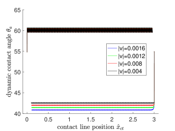
Figure 9 shows the effect of velocity on the dynamics. In these experiments, we fix , , and vary the dimensionless velocity from 0.02 to -0.02. As shown by the bottom three groups of curves in Figure 9, when , the contact angle decreases towards the receding angle and the contact line position moves to the negative direction. In the stick-slip stage, the effective contact line velocity in the averaged dynamic is exactly equal to the wall velocity . The effective receding angle also depends on . As turns smaller, the effective receding angle is closer to from below. In the case , the advancing dynamics is observed and increases until it starts to oscillate around the effect advancing angle. moves to the positive direction with an averaged velocity equal to . As turns smaller, the effective advancing angle is closer to from above. This validates our analysis made in Section 3.1. Moreover, the sensitivities of the effective receding and advancing contact angles to are different and asymmetric in this case.


Finally, we will study the effect of the geometric factor . We solve the problem (3.2) for two different choices of , which corresponds to the moving contact line problems in a microscopic channel () and on a moving fiber (). Figure 10 shows the dynamics of the advancing and receding angles. It is clear that the geometric factor affects the dynamic process, especially the first two stages. The contact angle approaches to its equilibrium value in the channel case much faster than that it does in the fiber case. However, the effective advancing and receding angles are the same in the two cases and they only depend on the dynamic factor , just as shown by the equation (3.13).


4.2 Comparison to experimental results
In this subsection, we will like to use our model and analysis to explain the experimental results of Guan et al. (2016a, b). There the dynamic contact angle hysteresis is observed by careful design of physical experiments. A very thin glass fiber with a inhomogeneous surface is inserted into a liquid reservoir. The fiber moves up and down so that a contact line moves on its surface. The capillary forces on the fiber are measured by AFM and the effective contact angles are computed. Several liquids with different surface tensions, viscosity and equilibrium angles are tested in their experiments. Many interesting phenomena are observed in the experiments. It is found that the dependence of the the advancing and receding contact angles on the fiber velocity is not unified (see Figure 6 in Guan et al. (2016b)). In some cases (e.g., the water-air system), the dependence of the advancing and receding contact angles on the velocity is very asymmetric. In some cases (e.g., the octanol-air system), this dependence seems symmetric. In some other cases (e.g., the FC77-air system), the advancing and receding contact angles are all very small and close to each other.
To compare with the experiments, we use the reduced model (2.29) which is an approximation for the problem in Guan et al. (2016b). We suppose the surface of the fiber is composed of two different materials and with different Young’s angles and . On the surface, the pattern of the Young’s angle is a piecewise constant periodic function with if and if , where is the percentage of material in a period. For the convenience in numerical computations, we smooth out this discontinuous pattern by a hyperbolic tangent function:
where is chosen to control the thickness of the smooth transition between two patterns. We use in our simulations. and can be chosen approximately according to the receding and advancing contact angles in the experiments with smallest velocity. We choose as a fitting parameter. The dimensionless wall velocity is represented by , where is in the reduced model (2.29).
The numerical results are given in Figure 11. We could see that the dependence of the contact angle hysteresis on the capillary number is not unified. For all the four cases, the advancing and receding contact angles and their dependence on the wall velocity are similar to that in the experiments in Guan et al. (2016a, b). In particular, it is found that the asymmetric dependence of the advancing and receding contact angles on the velocity can be weakened by increasing the proportion of the material with smaller contact angle in the patterned substrate. The numerical results also agree with the discussions in Subsection 3.3 based on the formula (3.13) of the effect contact angle. This also indicates that the experimental observations may be understood from our theoretical analysis in Section 3, especially the equation (3.13) on the effective contact angles. There we show that effective advancing and receding contact angles depend on the capillary number, the Young’s angles of the inhomogeneous substrate and also the spacial distributions of the patterns. All these parameters have important impacts and the interplay among them gives rise to very complicated experimental phenomena.


In real experiments, there are always thermal noises which affect the dynamics of the contact line. To make the numerical results more comparable with the experiments, we add a stochastic force in (2.18) to model other nondeterministic effects, e.g., thermal noises. The resulting stochastic system for the apparent contact angle and contact line position reads
| (4.1) |
This system of equations should be understood in the Itô sense. Since the contact angle and the contact line position are linked by the kinematic constraint (e.g., (2.20) and (2.27)) through the geometric factor , they are driven by the same Brownian motion . We assume the noise is small with so that it does not affect the dynamics too much. We then numerically solve (4.1) for one sample path using Euler-Maruyama scheme. Numerical results by solving the stochastic equation (4.1) are shown in Figure 12. We could see similar velocity dependence of the contact angle hysteresis as that in Figure 11 in the deterministic case. Moreover, the dynamic behaviours fit very well with the experiments for all the four cases, i.e, the water-air, octanol-air, decane-air, and FC77-air systems (Guan et al., 2016b).


In the end, we would like to remark that the previous comparisons with experiments are qualitative rather than quantitative, since there is a large gap between the capillary numbers chosen in our numerical simulation and those in the experiments. There are some issues which are not considered in our reduced model (2.29) (or (4.1)). For example, we assume that the contact line on the fiber is circular and the liquid-air interface is angular symmetric. The assumptions do not hold in experiments, where the chemical inhomogeneity is more complex on the fiber surface. The relaxation behaviour of the contact line is much more complicated on general surfaces than that in our model. The contact line hysteresis on general surfaces with chemical and geometrical roughness will be left for future work.
5 Conclusion
In this paper, we derive a formula (3.14) for the apparent contact angles on chemically inhomogeneous surfaces. It can be regarded as a Cox-type boundary condition for the time averaged apparent contact angle on these surfaces. The formula characterizes quantitatively how the averaged advancing and receding contact angles depend on the velocity, the Young’s angles and the distributions of the chemical inhomogeneities. It can be used to understand the complicated behavious for the dynamic contact angle hysteresis observed in experiments.
The derivation of the above formula is based on a reduced model for the macroscopic contact angle for moving contact line problems. The model is a leading order approximation for the famous Cox’s formula for small capillary number and is easier to analyze in the case with inhomogeneous surfaces. The reduced model is derived by using the Onsager principle as an approximation tool, which is much simpler than the standard asymptotic matching methods used in Cox (1986).
Although the main result is obtained by averaging the reduced model for a liquid-vapor system with small size, it can be generalized to other two-phase flow systems using the same averaging technique. In particular, it is straightforward to do averaging for the Cox’s boundary condition and derive a similar formula (3.17). These formulae can be used coupled with the standard two-phase Navier-Stokes equation. This will lead to a coarse-graining model for two-phase flow systems on chemical inhomogeneous surfaces. The dynamic contact angle hysteresis is given by the formulae and one does not need to resolve the microscopic inhomogeneity of the solid surfaces as in Yue (2020).
We mainly focus on the two-dimensional problem in the paper. But the results are useful for three dimensional problems when the inhomogeneity is simple. For example, when the defect is dilute, the static advancing and receding contact angles has been derived by Joanny & De Gennes (1984). Then it is possible to reduce the three dimensional problem into a two-dimensional one by symmetry assumptions. Thus one can apply the results in this paper to these problems. Some other problems may be handled in a similar way by combing our analysis with the modified Cassie-Baxter equation for static contact angle hysteresis in Choi et al. (2009); Xu & Wang (2013); Xu (2016).
For more general three-dimensional problems with rough or chemically inhomogeneous surfaces, the relaxation dynamics of the contact line is very complicated. the CAH may also depend on the depinning processes of a contact line even in quasi-static processes (Choi et al. (2009); Iliev et al. (2018)). For dynamical problems, the correlations and roughening processes of the contact line make the problem even more complicated (Golestanian & Raphaël (2003); Golestanian (2004)). Both the time averaging and the spacial homogenization needs to be considered simultaneously. The analysis for these problems will be left for future work.
Acknowledgments
The work of Z. Zhang was partially supported by the NSFC grant (No. 11731006, No. 12071207), the Guangdong Provincial Key Laboratory of Computational Science and Material Design (No. 2019B030301001), and the Guangdong Basic and Applied Basic Research Foundation (2021A1515010359). The work of X. Xu partially supported by the NSFC grant (No. 11971469) and by the National Key R&D Program of China under Grant 2018YFB0704304 and Grant 2018YFB0704300.
Declaration of Interests
The authors report no conflict of interest.
Appendix A Calculate the energy dissipation in a wedge region

Since we assume the region is in steady state, can be computed by solving the Stokes equation in the region. For simplicity, we can change variables and consider a problem as shown in Figure 13. We choose a polar coordinate system near the contact point. Let the contact point as the origin . The polar axis is in the right direction. In this system, the solid boundary will have a velocity , as shown in Figure 13. The viscous energy dissipation in the wedge region can be computed by solving the Stokes equations
| (A.1) |
and
| (A.2) |
We use no slip boundary condition on . The two-phase flow interface is assumed unchanged with time. Then the Stokes equation can be solved by the biharmonic equation.
We now calculate the dissipations in the wedge. To solve the problem, we apply the computations in Cox (1986). Introduce two stream functions and . We have
| (A.3) |
Here is the velocity in radial direction, and is the velocity in angular direction. Similar formula hold for . Then we have
| (A.4) |
The equations should satisfies the boundary conditions on the solid surface. We choose the no-slip boundary condition for the velocity except in the vicinity of the contact line when with the microscopic length is a cut-off parameter. When , we have
| (A.5) | |||
| (A.6) |
On the interface , we have
| (A.7) |
where .
The biharmonic equations in the wedge domains can be solved combining the above boundary and interface conditions. It leads to
| (A.8) | |||
| (A.9) |
Here the two group of coefficients are given by
and
Here
With the formula for and , we can compute the velocities in the two regions. For liquid A, we have
| (A.10) | |||
| (A.11) |
Then we have
| (A.12) |
where and are the unit vector in the radial and angular directions, respectively. We have similar representations for . The gradient of the velocity gives
| (A.13) |
Similarly,
| (A.14) |
Then the viscous energy dissipations in the wedge regions can be computed by
where is the cut-off parameter. Direct calculations lead to
| (A.15) |
Appendix B Properties of the averaged dynamics
In this section, we study the properties of the averaged dynamics (3.11) and (3.12). Without loss of generality, we assume . We also recall that is a nonnegative function satisfying and for , is a negative function bounded by and . We consider the behavior of the dynamic system for different regimes of starting at :
-
[i)]
-
1.
When , the averaged dynamic (3.12) is a good approximation. It yields the following properties:
-
(a)
monotonically decreases at a speed of at least until it arrives at .
This is because the harmonic average is positive when . As a result, we have
-
(b)
moves in the positive direction with a diminishing velocity.
In fact for , and as from the right. This can be shown in a similar way to that in the classical Laplace’s method in asymptotic analysis of integral. By expanding around its local maxima (which is a local minima of ), we have
where is a small positive number. As a result, diverges to as from the right.
-
(c)
approaches exponentially fast.
In fact, multiplying on both sides of Eq. (3.12a), we have
where and we have used the relation . An application of Gronwall’s inequality implies that
(B.1) It can be seen that decreases exponentially fast and arrives at at some finite time . Moreover, it is easily estimated that . The time period is a transient period for the dynamic of and .
-
(a)
-
2.
When , the effective dynamics follows (3.11) which yields the following properties:
-
(a)
The effective apparent contact angle decreases monotonically.
In fact, it is straightforward to show that and . Therefore, must arrive at at some finite time with .
-
(b)
The effective contact line position remains unchanged.
-
(a)
-
3.
When , the dynamics of the effective contact angle and contact point position are given by (3.12a) and (3.12b). This dynamic system has the following properties:
-
(a)
eventually arrives at a stable steady state satisfying .
In fact, and for . Since as from the left (similar to the proof in case (i)(b)), we also have when or . Then the equation has at least two roots in for small . As a result, the dynamics (3.12a) admits at least two steady state. As starts from in this regime, we are interested in the steady state closest to . We denote this state as .
is asymptotically stable or semi-stable if the right side of (3.12a) has non-positive derivative at . Since , direct calculation shows that this is equivalent to verify the derivative of is non-negative at (See Figure 14). This can also be proved by contradiction: suppose the derivative of is negative at , then is decreasing nearby , and we can find such that ; but this implies that there must be another root of in the interval by intermediate value theorem, which contradicts to the assumption that is the closest root to . Therefore, is a stable steady state.
-
(b)
Before achieving the steady state , continues decreasing due to the non-positiveness of the right side of (3.12a). Moreover, the effective contact line position moves to the negative direction since .
-
(c)
When arrives at the steady state , keeps on moving in the negative direction at a constant velocity .
-
(a)

Similar results hold in the case of . We can write the stable steady effective contact angle as a function of the drag velocity , i.e., . This function has the following properties:
-
1.
The steady effective contact angle must be outside the range of the chemical pattern : if , and is not far from , this is called receding contact angle; if , and is not far from , this is called advancing contact angle;
-
2.
as , while as . In other words, depending on different directions of the quasi-static motion, the steady effective contact angle approaches the lower bound or the upper bound of the chemical pattern.
This is a consequence of implicit function theorem and the smoothness of the function (See also Figure 7 for a sketch).
-
3.
In the extreme case , can be any value on the interval . This can be seen from the averaged dynamics (3.11a) and (3.12a) in three different cases: if the initial contact angle is larger than , then (B.1) with shows that the apparent contact angle decays exponentially to ; if the initial contact angle is smaller than , similar results hold that the apparent contact angle increases exponentially to ; if the initial contact angle is between and , then (3.11a) with implies that it is already equilibrium.
From these discussions, we can define the equilibrium apparent contact angle to be any value in the range when there is chemical roughness on the substrate. The contact line pins when ; the contact line advances if , while the contact line recedes if .
References
- Blake (2006) Blake, Terence D 2006 The physics of moving wetting lines. Journal of Colloid and Interface Science 299 (1), 1–13.
- Blake & De Coninck (2011) Blake, T. D. & De Coninck, Joël 2011 Dynamics of wetting and kramers’ theory. The European Physical Journal Special Topics 197 (1), 249–264.
- Bonn et al. (2009) Bonn, Daniel, Eggers, Jens, Indekeu, Joseph, Meunier, Jacques & Rolley, Etienne 2009 Wetting and spreading. Reviews of Modern Physics 81 (2), 739.
- Cassie & Baxter (1944) Cassie, A. & Baxter, S. 1944 Wettability of porous surfaces. Trans. Faraday Soc. 40, 546–551.
- Chan et al. (2020) Chan, T. S., Yang, F. & Carlson, A. 2020 Directional spreading of a viscous droplet on a conical fibre. Journal of Fluid Mechanics 894.
- Choi et al. (2009) Choi, W., Tuteja, A., Mabry, J. M., Cohen, R. E. & McKinley, G. H. 2009 A modified cassie-baxter relationship to explain contact angle hysteresis and anisotropy on non-wetting textured surfaces. J. Colloid Interface Sci. 339, 208–216.
- Cox (1983) Cox, RG 1983 The spreading of a liquid on a rough solid surface. Journal of Fluid Mechanics 131, 1–26.
- Cox (1986) Cox, R. 1986 The dynamics of the spreading of liquids on a solid surface. Part 1. Viscous flow. J. Fluid Mech. 168, 169–194.
- De Gennes (1985) De Gennes, Pierre-Gilles 1985 Wetting: statics and dynamics. Reviews of Modern Physics 57 (3), 827.
- Di et al. (2016) Di, Y., Xu, X. & Doi, M. 2016 Theoretical analysis for meniscus rise of a liquid contained between a flexible film and a solid wall. Europhys. Lett. 113 (3), 36001.
- Doi (2013) Doi, M. 2013 Soft Matter Physics. Oxfort University Press.
- Doi (2015) Doi, M. 2015 Onsager priciple as a tool for approximation. Chinese Phys. B 24, 020505.
- Doi et al. (2019) Doi, M., Zhou, J., Di, Y. & Xu, X. 2019 Application of the onsager-machlup integral in solving dynamic equations in nonequilibrium systems. Phys. Rev. E 99 (6), 063303.
- Dupont & Legendre (2010) Dupont, Jean-Baptiste & Legendre, Dominique 2010 Numerical simulation of static and sliding drop with contact angle hysteresis. Journal of Computational Physics 229 (7), 2453–2478.
- Dussan (1979) Dussan, EB 1979 On the spreading of liquids on solid surfaces: static and dynamic contact lines. Annual Review of Fluid Mechanics 11 (1), 371–400.
- E (2011) E, Weinan 2011 Principle of Multiscale Modeling. Cambridge University Press.
- Eggers (2005) Eggers, Jens 2005 Contact line motion for partially wetting fluids. Physical Review E 72 (6), 061605.
- Extrand (2002) Extrand, C. W. 2002 Model for contact angles and hysteresis on rough and ultraphobic surfaces. Langmuir 18, 7991–7999.
- Gao & McCarthy (2007) Gao, L. & McCarthy, T. J. 2007 How wenzel and cassie were wrong. Langmuir 23, 3762–3765.
- Gao & Wang (2012) Gao, Min & Wang, Xiao-Ping 2012 A gradient stable scheme for a phase field model for the moving contact line problem. Journal of Computational Physics 231 (4), 1372–1386.
- de Gennes et al. (2003) de Gennes, P.G., Brochard-Wyart, F. & Quere, D. 2003 Capillarity and Wetting Phenomena. Springer Berlin.
- Golestanian (2004) Golestanian, R. 2004 Moving contact lines on heterogeneous substrates. Phil. Trans. Roy. So. London. A 362 (1821), 1613–1623.
- Golestanian & Raphaël (2003) Golestanian, R. & Raphaël, E. 2003 Roughening transition in a moving contact line. Phys. Rev. E 67 (3), 031603.
- Guan et al. (2016a) Guan, D., Wang, Y., Charlaix, E. & Tong, P. 2016a Asymmetric and speed-dependent capillary force hysteresis and relaxation of a suddenly stopped moving contact line. Phys. Rev. Lett. 116 (6), 066102.
- Guan et al. (2016b) Guan, D., Wang, Y., Charlaix, E. & Tong, P. 2016b Simultaneous observation of asymmetric speed-dependent capillary force hysteresis and slow relaxation of a suddenly stopped moving contact line. Phys. Rev. E 94 (4), 042802.
- Guo et al. (2013) Guo, Shuo, Gao, Min, Xiong, Xiaomin, Wang, Yong Jian, Wang, Xiaoping, Sheng, Ping & Tong, Penger 2013 Direct measurement of friction of a fluctuating contact line. Physical Review Letters 111 (2), 026101.
- Guo et al. (2019) Guo, S., Xu, X., Qian, T., Di, Y., Doi, M. & Tong, P. 2019 Onset of thin film meniscus along a fibre. J. Fluid Mech. 865, 650–680.
- Gurtin et al. (1996) Gurtin, Morton E, Polignone, Debra & Vinals, Jorge 1996 Two-phase binary fluids and immiscible fluids described by an order parameter. Mathematical Models and Methods in Applied Sciences 6 (06), 815–831.
- Haley & Miksis (1991) Haley, Patrick J & Miksis, Michael J 1991 The effect of the contact line on droplet spreading. Journal of Fluid Mechanics 223, 57–81.
- Huh & Scriven (1971) Huh, C. & Scriven, L.E. 1971 Hydrodynamic model of steady movement of a solid/liquid/fluid contact line. J. colloid Interface Sci. 35 (1), 85–101.
- Iliev et al. (2018) Iliev, Stanimir, Pesheva, Nina & Iliev, Pavel 2018 Contact angle hysteresis on doubly periodic smooth rough surfaces in wenzel’s regime: The role of the contact line depinning mechanism. Physical Review E 97 (4), 042801.
- Jacqmin (2000) Jacqmin, D. 2000 Contact-line dynamics of a diffuse fluid interface. J. Fluid Mech. 402, 57–88.
- Joanny & Robbins (1990) Joanny, J. & Robbins, M. 1990 Motion of a contact line on a heterogeneous surface. J. Chem. Phys 92 (2), 32063212.
- Joanny & De Gennes (1984) Joanny, J. F. & De Gennes, P.-G. 1984 A model for contact angle hysteresis. J. Chem. Phys. 81 (1), 552–562.
- Johnson Jr. & Dettre (1964) Johnson Jr., R. E. & Dettre, R. H. 1964 Contact angle hysteresis. iii. study of an idealized heterogeneous surfaces. J. Phys. Chem. 68, 1744–1750.
- Man & Doi (2016) Man, X. & Doi, M. 2016 Ring to mountain transition in deposition pattern of drying droplets. Phys. Rev. Lett. 116 (6), 066101.
- Marmottant & Villermaux (2004) Marmottant, Philippe & Villermaux, Emmanuel 2004 On spray formation. Journal of Fluid Mechanics 498, 73–111.
- Marmur & Bittoun (2009) Marmur, A. & Bittoun, E. 2009 When wenzel and cassie are right: Reconciling local and global considerations. Langmuir 25, 1277–1281.
- Miskis & Davis (1994) Miskis, M. J. & Davis, S. H. 1994 Slip over rough and coated surfaces. Journal of Fluid Mechanics 273, 125–139.
- Neumann & Good (1972) Neumann, A. W. & Good, R. J. 1972 Thermodynamics of contact angles: I. heterogeneous solid surfaces. J. Colloid Interface Sci. 38, 341–358.
- Pavliotis & Stuart (2008) Pavliotis, G. A. & Stuart, A. M. 2008 Multiscale Methods: Averaging and Homogenization. New York: Springer.
- Pismen (2002) Pismen, LM 2002 Mesoscopic hydrodynamics of contact line motion. Colloids and Surfaces A: Physicochemical and Engineering Aspects 206 (1), 11–30.
- Pismen & Pomeau (2000) Pismen, Len M & Pomeau, Yves 2000 Disjoining potential and spreading of thin liquid layers in the diffuse-interface model coupled to hydrodynamics. Physical Review E 62 (2), 2480.
- Prabhala et al. (2013) Prabhala, B., Panchagnula, M. V. & Vedantam, S. 2013 Three-dimensional equilibrium shapes of drops on hysteretic surfaces. Colloid Polym. Sci. 291, 279–289.
- Priest et al. (2007) Priest, C., Sedev, R. & Ralston, J. 2007 Asymmetric wetting hysteresis on chemical defects. Phys. Rev. Lett. 99 (2), 026103.
- Qian et al. (2003) Qian, T., Wang, X.P. & Sheng, P. 2003 Molecular scale contact line hydrodynamics of immiscible flows. Phys. Rev. E 68, 016306.
- Qian et al. (2006) Qian, T., Wang, X.P. & Sheng, P. 2006 A variational approach to moving contact line hydrodynamics. J. Fluid Mech. 564, 333–360.
- Raj et al. (2012) Raj, R., Enright, R., Zhu, Y., Adera, S. & Wang, E. N. 2012 Unified model for contact angle hysteresis on heterogeneous and superhydrophobic surfaces. Langmuir 28, 15777–15788.
- Raphael & de Gennes (1989) Raphael, Elie & de Gennes, Pierre-Gilles 1989 Dynamics of wetting with nonideal surfaces. the single defect problem. The Journal of chemical physics 90 (12), 7577–7584.
- Ren & E (2007) Ren, W. & E, W. 2007 Boundary conditions for the moving contact line problem. Phys. Fluids 19 (2), 022101.
- Ren & E (2011) Ren, W. & E, W. 2011 Contact line dynamics on heterogeneous surfaces. Phys. Fluids 23, 072103.
- Ren et al. (2015) Ren, Weiqing, Trinh, P. H. & E, Weinan 2015 On the distinguished limits of the navier slip model of the moving contact line problem. Journal of Fluid Mechanics 772, 107–126.
- Renardy et al. (2001) Renardy, Michael, Renardy, Yuriko & Li, Jie 2001 Numerical simulation of moving contact line problems using a volume-of-fluid method. Journal of Computational Physics 171 (1), 243–263.
- Schwartz & Eley (1998) Schwartz, Leonard W & Eley, Richard R 1998 Simulation of droplet motion on low-energy and heterogeneous surfaces. Journal of Colloid and Interface Science 202 (1), 173–188.
- Schwartz & Garoff (1985) Schwartz, L. W. & Garoff, S. 1985 Contact angle hysteresis on heterogeneous surfaces. Langmuir 1, 219–230.
- Seppecher (1996) Seppecher, Pierre 1996 Moving contact lines in the Cahn-Hilliard theory. International Journal of Engineering Science 34 (9), 977–992.
- Seveno et al. (2009) Seveno, David, Vaillant, Alexandre, Rioboo, Romain, Adao, H, Conti, J & De Coninck, Joël 2009 Dynamics of wetting revisited. Langmuir 25 (22), 13034–13044.
- Shikhmurzaev (1993) Shikhmurzaev, Y. D. 1993 The moving contact line on a smooth solid surface. Inter. J. Multiphase Flow 19 (4), 589–610.
- Sibley et al. (2015) Sibley, D. N., Nold, A. & Kalliadasis, S. 2015 The asymptotics of the moving contact line:cracking an old nut. J. Fluid Mech. 764, 445–462.
- Snoeijer & Andreotti (2013) Snoeijer, J. H. & Andreotti, B. 2013 Moving contact lines: scales, regimes, and dynamical transitions. Annual Rev. Fluid Mech. 45, 269–292.
- Spelt (2005) Spelt, Peter DM 2005 A level-set approach for simulations of flows with multiple moving contact lines with hysteresis. Journal of Computational Physics 207 (2), 389–404.
- Sui et al. (2014) Sui, Y., Ding, H. & Spelt, P. 2014 Numerical simulations of flows with moving contact lines. Annual Rev. Fluid Mech. 46, 97–119.
- Sui & Spelt (2013a) Sui, Yi & Spelt, Peter DM 2013a An efficient computational model for macroscale simulations of moving contact lines. Journal of Computational Physics 242, 37–52.
- Sui & Spelt (2013b) Sui, Yi & Spelt, Peter DM 2013b Validation and modification of asymptotic analysis of slow and rapid droplet spreading by numerical simulation. Journal of Fluid Mechanics 715, 283–313.
- Tanner (1979) Tanner, L.H. 1979 The spreading of silicone oil drops on horizontal surfaces. Journal of Physics D: Applied Physics 12 (9), 1473.
- Wang et al. (2008) Wang, X.P., Qian, T. & Sheng, P. 2008 Moving contact line on chemically patterned surfaces. J. Fluid Mech. 605, 59–78.
- Wenzel (1936) Wenzel, R. N. 1936 Resistance of solid surfaces to wetting by water. Ind. Eng. Chem. 28, 988–994.
- Whyman et al. (2008) Whyman, G., Bormashenko, E. & Stein, T. 2008 The rigorous derivative of young, cassie-baxter and wenzel equations and the analysis of the contact angle hysteresis phenomenon. Chem. Phy. Letters 450, 355–359.
- Xu (2016) Xu, X. 2016 Modified wenzel and cassie equations for wetting on rough surfaces. SIAM J. Appl. Math. 76 (6), 2353–2374.
- Xu et al. (2016) Xu, X., Di, Y. & Doi, M. 2016 Variational method for contact line problems in sliding liquids. Phys. Fluids 28, 087101.
- Xu & Wang (2020) Xu, Xianmin & Wang, Xiaoping 2020 Theoretical analysis for dynamic contact angle hysteresis on chemically patterned surfaces. Physics of Fluids 32 (11), 112102.
- Xu & Wang (2011) Xu, X. & Wang, X. P. 2011 Analysis of wetting and contact angle hysteresis on chemically patterned surfaces. SIAM J. Appl. Math. 71, 1753–1779.
- Xu & Wang (2013) Xu, X. & Wang, X. P. 2013 The modified cassie’s equation and contact angle hysteresis. Colloid Polym. Sci. 291, 299–306.
- Xu et al. (2019) Xu, X., Zhao, Y. & Wang, X.-P. 2019 Analysis for contact angle hysteresis on rough surfaces by a phase field model with a relaxed boundary condition. SIAM J. Appl. Math. 79, 2551–2568.
- Young (1805) Young, T. 1805 An essay on the cohesion of fluids. Philos. Trans. R. Soc. London 95, 65–87.
- Yue (2020) Yue, Pengtao 2020 Thermodynamically consistent phase-field modelling of contact angle hysteresis. Journal of Fluid Mechanics 899.
- Yue & Feng (2011) Yue, P. & Feng, J. J. 2011 Can diffuse-interface models quantitatively describe moving contact lines? The European Physical Journal Special Topics 197 (1), 37–46.
- Zhang & Yue (2020) Zhang, Jiaqi & Yue, Pengtao 2020 A level-set method for moving contact lines with contact angle hysteresis. Journal of Computational Physics p. 109636.
- Zhang & Ren (2019) Zhang, Zhen & Ren, Weiqing 2019 Distinguished limits of the navier slip model for moving contact lines in stokes flow. SIAM Journal on Applied Mathematics 79, 1654–1674.
- Zhou & Doi (2018) Zhou, J. & Doi, M. 2018 Dynamics of viscoelastic filaments based on onsager principle. Phys. Rev. Fluids 3 (8), 084004.
- Zhou & Sheng (1990) Zhou, Min-Yao & Sheng, Ping 1990 Dynamics of immiscible-fluid displacement in a capillary tube. Physical Review Letters 64 (8), 882.