Effect of topological length on Bound states signatures in a Topological nanowire
Abstract
Majorana bound states (MBS) at the end of nanowires have been proposed as one of the most important candidate for the topological qubits. However, similar tunneling conductance features for both the MBS and Andreev bound states (ABS) have turned out to be a major obstacle in the verification of the presence of MBS in semiconductor-superconductor heterostructures. In this article, we use a protocol to probe properties specific to the MBS and use it to distinguish the topological zero-bias peak (ZBP) from a trivial one. For a scenario involving quantized ZBP in the nanowire, we propose a scheme wherein the length of the topological region in the wire is altered. The tunneling conductance signatures can then be utilized to gauge the impact on the energy of the low-energy states. We show that the topological and trivial ZBP behave differently under our protocol, in particular, the topological ZBP remains robust at zero bias throughout the protocol, while the trivial ZBP splits into two peaks at finite bias. This protocol probes the protection of near zero energy states due to their separable nature, allowing us to distinguish between topological and trivial ZBP.
I Introduction
The Kitaev’s one-dimensional topological superconducting model [1] predicts Majorana modes at the ends of the 1D chain. These well separated states form robust nonlocal fermionic states and in addition under braiding the Majorana states obey non-abelian statistics, thus potentially providing an ideal base for fault-tolerant topological quantum computation [2, 3, 4]. Since then number of theoretical proposals have been made for potentially realizing systems that could host the Majoranas. Some of the earliest proposals include, fractional quantum Hall states at filling [5], spinless topological superconductors with the cores hosting Majoranas [6]. Others include, the cores of superconducting vortices present on the surface of a 3D topological insulator proximitized to s-wave superconductor [7], a semiconductor film with spin-orbit interaction and proximity coupled to an s-wave superconductor and magnetic field [8], in a quantum-wire with strong spin-orbit interaction proximity coupled to superconductor in the presence of magnetic-field [9, 10] which drives the system from a trivial phase with a finite gap to a topological phase containing a zero-energy MBS in the gap. Intensive experimental efforts have been made on realizing the above setups, in particular the last setup involving InAs, InSb, etc., quantum wires have been quite promising [11, 12, 13, 14]
Of all the signatures of MBS, the overwhelming emphasis has been on experimentally detecting the zero-bias tunneling conductance and their corresponding interpretation [15, 16, 17, 18, 19, 20, 21, 22, 23, 24, 25, 26, 27, 28, 29, 30, 31, 32, 33, 34, 35, 36, 37, 38, 39, 40, 41, 42, 43]. From the theoretical perspective, tunneling at the edge of the topological superconductor (where the MBS are localized) results in a resonant effect, consequently the Zero-bias peak (ZBP) conductance is expected to acquire the quantized value of [15]. Previous studies have shown that the ZBP can also appear due to the Andreev bound states (ABS), with the peak height close to the quantization values [25, 26, 18]. The origin of ABS is often due to inhomogeneous profiles and quantum dots at the wire’s end and many a times they mimic MBS’s tunneling signatures.
The typical ABS consists of overlapping Majorana components, making them very sensitive to parameter changes. Therefore, the ZBP due to the ABS can generally be attributed to the fine tuning of the parameters and hence not robust [44]. Recent theoretical works have shown that the trivial in-gap states can actually be pinned close to zero energy for an extended range of parameter space for certain inhomogeneous profiles, making the ZBP robust. These ABS have their Majorana components partially separated (termed as the ps-ABS) from each other [45]. On the other hand, for magnetic field strengths greater than the critical value, the wire will be in the topological regime wherein the Majorana components are completely separated and localized at the two ends of the wire. It turns out that the ps-ABS appear just before the critical Zeeman term, thus it is challenging to unambiguously pin the origin of the ZBP as arising from either the topological or the trivial states.
To distinguish them, use of two leads each placed at the opposite ends of the wire have been proposed as they can measure the correlations between the conductance from the two local leads. In addition, this setup can be used to probe non-local conductances which arise due to the bulk states and can produce the band gap closing signature at the topological phase transition point beyond which MBS appears [44, 46].
However, as discussed in Refs.[47], the presence of inhomogeneities like quantum dots at both the ends can yield correlated trivial ZBP in both the local conductances. It turns out that the non-local conductance signatures in case of the heterostructures are not strong enough to unambiguously depict the band gap closing. Besides the above, dephasing, leakage dynamics of Majorana [48] and recent studies focused on the robustness of quantization of ZBP with respect to tunneling barrier height and temperature [49] have been suggested as potential schemes to distinguish the topological Majorana modes from the Andreev states.
As mentioned in the preceding paragraph the presence of quantized ZBP is insufficient to conclude the existence of MBS as trivial ABS can also produce quantized ZBP. To distinguish topological states from normal zero-modes, one needs to go beyond the presence of Quantized ZBP and probe properties specific to MBS only. Consider that the ends of a wire are moved into trivial parameter space by changing the topological length of the wire; in such a case, one produces a trivial-topological-trivial structure with the MBS still present at the edge of the topological region. This property specific to the MBS has been proposed before for Majorana braiding protocols [50, 51, 52, 53]. Motivated by this, we define the “moving protocol” to systematically decrease the topological length by fixing the wire’s ends in a parameter regime below the topological range by either reducing the Zeeman term or the external potential. We employ “Zeeman moving protocol” (ZMP) by applying Zeeman term profile and “Potential moving protocol” (PMP) with external potential in our numerical simulation. Since local conductance measures the local property of the wire close to the lead, the effect of change in the topological region should be apparent in the local conductance. We apply both the protocol to diverse scenarios and investigate their impact on the trivial and the topological ZBP. We show that the topological ZBP from MBS remains robust under the moving protocol. At the same time, the trivial ZBP from ps-ABS has entirely different behaviour, splitting into two separate peaks at finite bias. This difference in behavior arises due to the fundamental difference between the MBS and ps-ABS in the overlap of their Majorana components. Our “moving protocol” indirectly probes this separable nature of the Majorana components. We also show that the PMP is more effective compared to ZMP as far as distinguishing trivial and topological ZBPs are concerned, moreover, the practical implementation of this scheme is also relatively more feasible.
The organization of the paper is as follows. In section II, we describe the model and profile of the semiconductor-superconductor nanowire used to produce the different heterostructures. In this section, we also define our moving protocols, under which we will study tunneling conductance signatures. In section III, we present our results. First, we look into a homogeneous nanowire and its tunneling conductance signatures. We also look at the inhomogeneous system, which can have both trivial and topological ZBP. We show the effect of ZMP on the trivial and topological ZBP to demonstrate the different ways they behave. In subsection III.3, we present the behaviour of topological and trivial ZBP under PMP. In subsection III.4, we consider another system, S′SS′ (where S′ and S are superconducting region of the wire with different chemical potential) system to showcase the shortcomings of the ZMP and how we go around it by using the PMP to distinguish topological ZBP from trivial ZBP. Finally, we present our conclusions in section IV.
II Model
We study a 1D semiconductor nanowire with spin-orbit coupling having a superconducting gap induced via the proximity effect. In addition, we take into consideration magnetic field applied parallel to the wire. The corresponding Hamiltonian which incorporates all of the above terms is given by
| (1) | |||||
where () represents creation (annihilation) operators of fermions with spin at site . The parameters , , , and represent the tunneling, spin-orbit, chemical potential, Zeeman energy and the superconducting terms, respectively at the site . This will be our base model on top of which different profiles of and are added to create different heterostructures.
We will focus our attention to the following two scenarios. The first one is the homogeneous case in which all the parameters in the Hamiltonian are taken to be position independent. We reproduce the result of this well studied parameter regime to validate our numerical scheme and to interpret the effect of our protocol on this system. In the second scenario we will consider the presence of smooth variation in the and profiles. The latter differentiates the different chemical potenital in the normal (N) regions and the superconductor (S) regions, while the former creates regions of N and S resulting in NS and NSN type of heterostructures. For certain parameter regimes these heterostructures can host ABS or quasi-MBS which can stay close to zero energy over large range of magnetic fields. The smooth variation of the spatial profile is modeled by the function [47, 46, 44]
| (2) |
where represents the point around which the profile changes, while is a measure of smoothness in the variation (which has been fix to for all profiles).
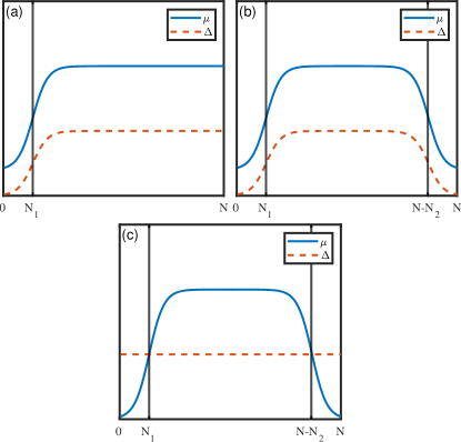
For example, an NS profile with smoothly varying chemical potential can be represented via the following set of parameters
| (3) |
where is the length of the Normal region in the heterostructure, and are the chemical potential for the S and N regions respectively, and is the effective superconducting coupling strength in the S region. The NSN heterostructure can be modeled by the following set of parameters with the profile given by
| (4) |
where and are the chemical potentials for the Normal regions. we note that , and , denote the length of left and right normal regions and the superconducting region respectively. Together with these systems we also consider S′SS′ which has a homogeneous but inhomogenity in , which distinguish the two superconducting region S′ and S.
| (5) |
Plots of the NS, NSN and S′SS′ systems and profile are shown in Fig. 1.
As a simple diagnostic tool to distinguish the presence of MBS from the ABS in the various parameter regimes we calculate the boundary topological invariant (TI) using the scattering matrix . The scattering matrix relates the incoming and the outgoing wave amplitudes
| (6) |
Note that the reflection subblocks and the transmission subblocks connects the two ends of the chains and are obtained in terms of the Fermi level wave amplitudes. The TI , obtains a value when the wire is in the trivial phase and for the topological phase [54], further details are provided in Appendix A. Along with the topological invariant we also plot the wavefunction of the Majorana components to characterise the topological nature of the bound states. The Hamiltonian has particle-hole symmetry, giving rise to symmetric spectrum with two fermionic wave functions and for every eigenvalue . Thus one constructs the following symmetric and anti-symmetric wave functions from the low energy eigenstates
| (7) |
The wire can thus be characterised as topological (with MBS) if and are spatially separated, while the overlapping and partially overlapping states characterises ABS and ps-ABS, respectively [44, 49].
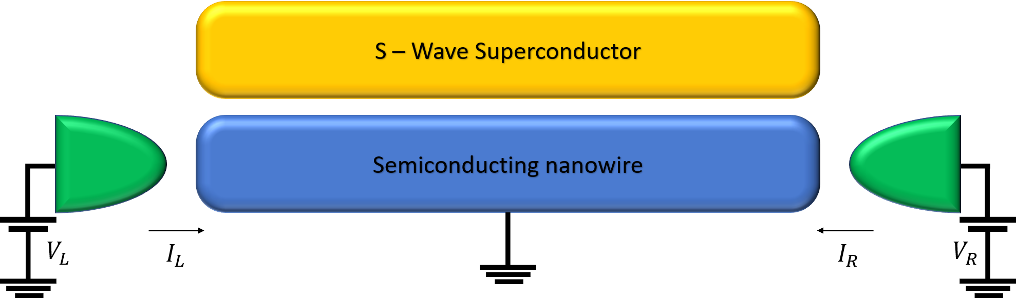
We perform tunneling conductance calculations for a setup involving two normal leads attached to either side of the wire to create a three terminal device (see Fig. 2)[46]. The conductance matrix has the following form
| (8) |
where the elements of the matrix are given by
| (9) |
The local and the non-local conductance are calculated using the Green’s function method. Details related to the calculations are provided in the Appendix B. We focus our attention on the effect the topological length of the wire has on the tunneling conductance signatures. By appropriately choosing site-dependent Zeeman or the chemical potential terms, different regions of the 1D wire can be tuned to be in the topological or the trivial phase [50, 51]. Consider the following spatial dependent Zeeman strength
where
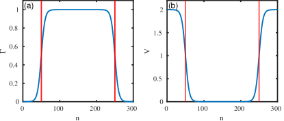
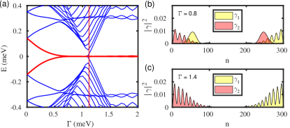
and here represents the full length/site of the nanowire and is smoothness parameter (fixed to ). A sample plot of the profile is shown in Fig. 3(a) for . For the protocol that we consider, is kept unchanged while is increased from negative to positive values. If is above the critical field, the wire will be topological for approximately regions. Thus, increasing decreases the length of the topological region due to the Zeeman strength being below the critical values in those regions. For this profile creates a domain wall structure of trivial-topological-trivial superconductor, changing thus results in the change of the topological length. We denote this protocol of changing the topological length as the “Zeeman Moving protocol” (ZMP) and we will be exploring the effect it has on the ZBP due to the presence of either the ps-ABS or the MBS. In addition to the Zeeman term, one could also use tunable local gates to add an external potential which increases the effective chemical potential in the ends of the wire to put them in a trivial state, thus decreasing the topological length. To consider this we will add external potential of the form Eq. (10) to our chemical potential the plot of which is shown in Fig. 3(b). We denote this protocol of changing the topological length as the “Potential Moving protocol” (PMP).
| (10) |
III Results
In this section, we will be considering the effects of the moving-protocol on the ZBP for the homogeneous and inhomogeneous systems. For either of them, we begin by exploring the phase diagram by calculating the topological boundary invariant. Further, we calculate the Majorana components to classify the in-gap states. We reproduce some of the earlier results on the ZBP by calculating the tunneling conductance. The main thrust of our work is to distinguish the ZBP arising due to the presence of topological and trivial bound states via the moving protocol.
III.1 Homogeneous System
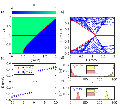
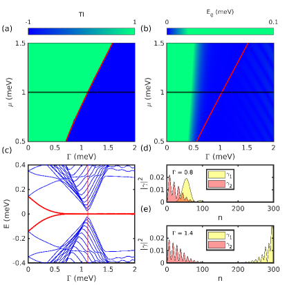
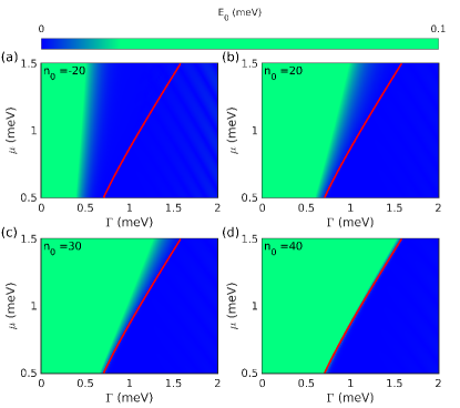
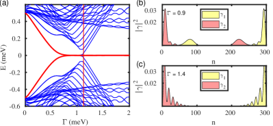
We choose the parameter space of InSb-Al nanowire that are often used in theoretical and experimental studies[44, 46]. The effective mass considered is with lattice constant nm and Rashba spin orbit coupling eV which yields meV and meV. The effective superconducting coupling term considered is meV [49, 46]. The ideal system enters the topological non-trivial region when the Zeeman strength is greater than the critical value given by . Using the scattering matrix approach we have calculated the TI for a range of and , and as shown in Fig. 4(a) the numerically obtained boundary between the topological and the non-topological region coincides with the theoretical prediction of the critical field shown by the red curve. For concretness, we consider meV as the onsite potential, the corresponding critical Zeeman strength for which the band closing takes place is meV. From the plot of energy spectrum Vs shown in Fig. 4(b), we observe the expected appearance of zero energy modes after the band closing which takes place at the critical Zeeman field.
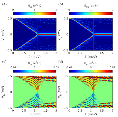
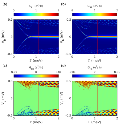
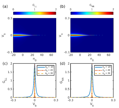
The numerically calculated tunneling conductance for a range of is plotted in Fig. 5. It is clear from the figure that ZBP in the local conductance appears after . The ZBP is quantized at which is also the predicted conductance for the MBS. The left() and right() local conductances exhibit coherence denoting the presence of MBS on either ends of the nanowire and at the same time the non-local conductance and exhibit the signature of band gap closing. These tunneling conductance signatures arising from a ideal nanowire with MBS at the edges of the pristine nanowire have been well studied in the past literature [49, 46].
Before we discuss the effect of the ZMP on the ZBP, we will first explore its effect on the system’s energy levels. Results of spectrum under ZMP for two different values of are shown in Fig. 4(c). From the plot of the energy spectrum it is clear that the MBS remain fixed at the zero energy since the protocol only changes the length of the topological region by putting some part of the wire in a Zeeman term below the critical term(). As long as the length of the topological region remains much larger than the Majorana localization length, the energies of the MBS will be fixed at zero energy due to the topological protection. Further insight into the effect of the protocol on the state is obtained by plotting the Majorana components of the low energy states. For uniform Zeeman term (which is the case for ) the MBS are localized at the edges of the nanowire with the two Majorana components spatially separated (see Fig. 4(d)). However, as the Zeeman term profile is moved so that , the length of the topological region as well as the bound state position changes but at the same time they remain localized at the edges of the topological region as shown in Fig. 4(e). The Majorana components are still separated so they stay at zero energy.
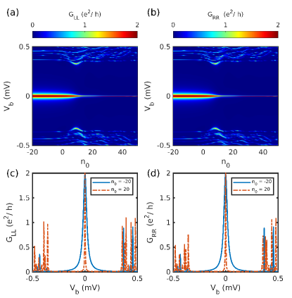
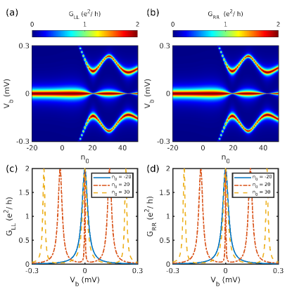
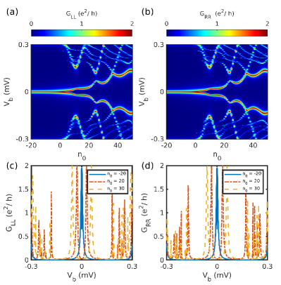
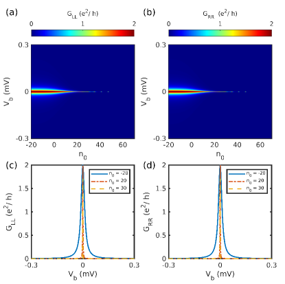
We next focus the effect of ZMP on the ZBP. For the ZMP, the calculated local conductance for a range of can be seen in Figs. 6(a-b). As is increased (i.e., the topological region is reduced while the position of the lead remains unchanged), a subsequent decrease in the width of the ZBP becomes apparent, while at the same time the height of the peak remains quantized to the value . We also plot value of the conductance for two values of in Figs. 6(c-d), where the quantization of peak is clearly observed. This feature has a simple explanation due to the property of the MBS. Application of the moving protocol changes the topological length of the wire and therefore the MBS moves further away from the lead while always staying at the edge of the topological region. Since the edge states move further away from the lead the coupling between the lead and the MBS decreases, resulting in the reduced width of the ZBP. For sufficiently large separation between the lead and the edge mode, the ZBP disappears altogether. Through out this protocol the Majorana components remain spatially separated, as a result the MBS remains at the zero energy causing the peak to be at zero bias through out this protocol.
III.2 Inhomogeneous Wire
In quantum wires it is difficult to achieve a scenario wherein the parameters are homogeneous through out the length of the wire. Instead, the inhomogeneous profile in the heterostructure better captures the realistic scenario. We begin by considering an inhomogeneous NS heterostructure where the chemical potential and the superconducting profile used to model the heterostructure is given by Eq. (3) and shown in Fig. 1(a). The numerically calculated topological boundary invariant is shown in Fig. 7(a), which shows the presence of topological phase for Zeeman terms greater than for a given value of the chemical potential (in the region). This figure is similar to the corresponding Fig. 4(a) for the homogeneous case. However, the difference between the two scenarios can be seen from the presence of low lying energy states close to zero energy even in the non-topological regime , see Fig. 7(b). It turns out that the zero energy modes in the trivial region persist for large range of Zeeman coupling and chemical potential. The energy spectrum for the system for meV is shown in Fig. 7(c), which shows the appearance of ABS before the topological phase transition at meV. For the Majorana components obtained from the low-lying states are localized in non-overlapping regions (at the edges) and are the MBS (see Fig. 7(e)), while for the components have significant overlap with each other and are the partially separated ABS, as shown in Fig. 7(d).
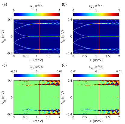
Consider next the Fig. 8 which depicts the tunneling conductance calculated for the NS heterostructure. For (denoted by the red vertical line) both the local conductances, and , exhibit ZBP with a peak height of which is consistent with the presence of MBS. It turns out that for the left lead this signature of MBS persists even for extended values of . The trivial ZBP has a splitting at zero energy, however, the splitting is negligible making it difficult to resolve even at low non-zero temperatures [55, 56]. Another aspect which is different from the signatures in the topological regime is the absence of a ZBP on the right tunneling conductance (see Fig. 8(b)). The reason for this is the presence of bound states only on the left side of the wire, which couples to the corresponding left lead only. The absence of correlation in the local conductance is associated with the signature of ABS [44]. As for the non-local conductance, the plots in Figs. 8(c-d) exhibit weak signature to unambiguously distinguish bulk gap closing at . Similar results for NS heterostructure have been demonstrated previously in the literature[47, 46].
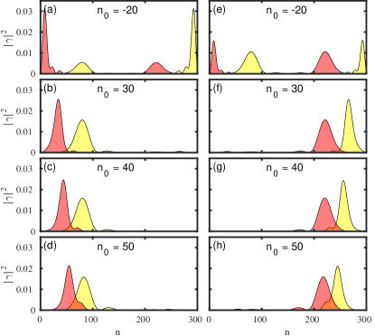
In this scenario where the tunneling setup involves two leads it is more likely that the inhomogeneity will be present on both sides of the nanowire. The profile used to reproduce the NSN heterostructure is given in Eq. (4) and shown in Fig. 1(b). We find that for a range of parameters the NSN structure also hosts ABS. The same is verified from the energy spectrum in Fig. 9(a), with ABS appearing much before the critical Zeeman term similar to that for the NS system. Even if the energy spectrum for both the systems are nearly the same, the difference between the two can be seen from the Majorana component plots for the zero energy modes as shown in Fig. 9(b). For the NSN heterostructure the bound states for are also localized at both ends just like the MBS. These bound states are the ps-ABS, with the partially separated Majorana components at both ends of the wire.
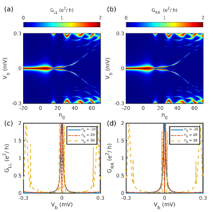
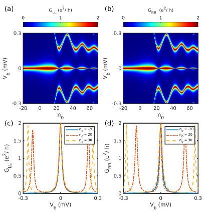
The tunneling conductance of the NSN heterostructure is shown in Fig. 10. Now both the left () and the right () local conductance exhibit quantized ZBP and are also correlated. As before, these signatures are present even for . However, even for this system the non-local conductance is unable to capture the band gap closing. This can again be attributed to the bulk states being localized in the superconducting region. Thus the correlated quantized ZBP produced by the ps-ABSs and the absence of band gap signature implies no distinguishing feature between the ABS and the MBS. These conclusions were reported previously by Hess et. al. [47].
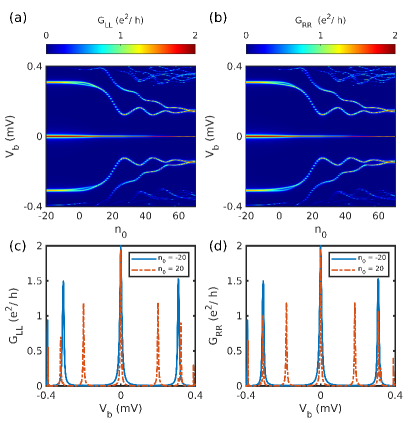
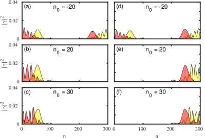
We will now present the effect of ZMP on the trivial and topological ZBP for the inhomogeneous system. As we saw before, the NS system has both the topological and trivial quantized ZBP. The quantized ZBP for is present in both the left and the right local conductance, which on the application of ZMP persists for a range of values. This result is similar to the case of homogeneous wire with topological ZBP as discussed in Sec. III.1 . Interestingly, effect of ZMP on the trivial ZBP present on the left conductance for the NS system is significantly different (see Fig. 12). The ZBP splits into two separate peaks as increases. As discussed before, the topological and trivial peak for the NSN system is the most challenging to distinguish. So we apply ZMP to the tunneling conductance signature to the NSN system. The topological ZBP persists for an extended range of , and the peak width decreases with an increase in as is the case for the NS system (see Fig. 13). In contrast, under ZMP, the trivial ZBP present on both local conductances splits into two separate peaks as shown in Fig. 14.
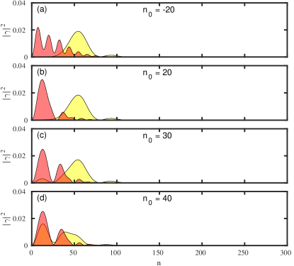
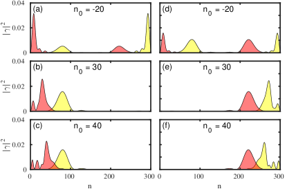
To get an insight into the behavior of topological and trivial peaks under the moving protocol, we focus our attention on the Majorana components of the state close to zero energy. Figure 15 shows the effect of ZMP on the Majorana components of the trivial states close to zero energy for the NS system. The trivial ZBP originates due to the ps-ABS which involves partially separated Majorana components. Under the application of ZMP, the overlap between the Majorana components increases, causing them to acquire a finite energy split, resulting in splitting of the ZBP into two peaks away from zero bias. For the case of NSN heterostructure we have two states close to zero energy, both of which are present at either ends of the wire. These states are ps-ABSs with small overlapping Majorana components. On the application of ZMP, the overlap increases for both the states (see Fig. 17), resulting in a finite energy split and the trivial ZBP on both local conductances splits into two separate peaks at finite bias.
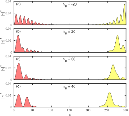
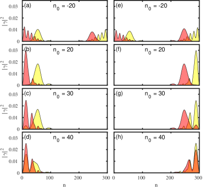
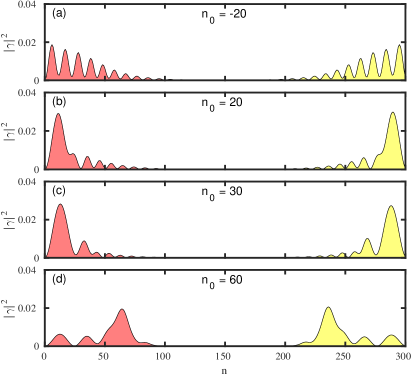
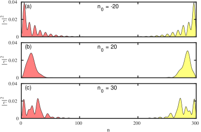
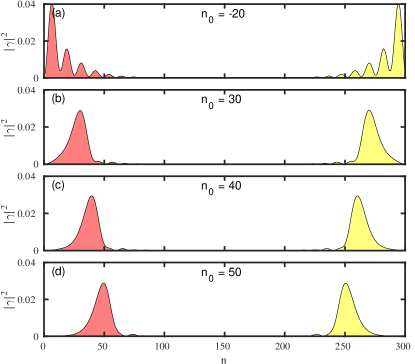
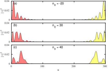
Performing similar analysis for the topological states, we show the effect of ZMP on the Majorana components of MBS in NS and NSN systems in Fig. 16 and Fig. 18, respectively. Fully separated Majorana components represent the MBS, and the components remain separate throughout the protocol for both the NS and NSN systems. As a result, the MBS stays at zero energy resulting in the ZBP staying at zero bias throughout the protocol. Under the protocol, the components move away from the edge (see Fig. 18), resulting in weak coupling with the leads, leading to decreased peak width. For a large value(), the states will be far from the edge, making the peak disappear. Another thing to notice is that the decrease in peak height on both the local conductances of NS is different under the protocol as shown in Fig. 11(a-b). This is mainly due to the presence of the N region on the left side and MBS leaking to this region, see Fig. 18.
To showcase that the robustness of MBS energy to ZMP and the splitting is present for all parameter range of ABS, we plot the phase potrait corresponding to the lowest energy eigenvalues for the parameter range with the ZMP for different values. As shown in Fig. 19, with we have normal NSN system with low energy ABS present before the topological region (separated by red line) with the application of the ZMP these low energy states moves away from zero energy and for there are no zero energy states outside the topological region. These plots show that the splitting is not specific to certain parameter values and the ABS move away from zero energy for all the parameter ranges. On the other hand the eigenvalues of the MBS in the topological region remains unaffected.
III.3 Moving protocol with external potential
As discussed in Sec. II, external potential can also be used to modify the topological length of a nanowire and produce a trivial-topological-trivial structure. In earlier works, this strategy has been suggested in the context of braiding protocol [50, 51, 52, 53]. However, a moving protocol with tunneling measurements at the edges has not been considered before for the purpose of distinguishing topological states from trivial ones. In this subsection we will be presenting the effect of the PMP on trivial and topological ZBP.
III.3.1 Homogeneous wire
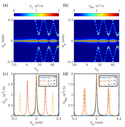
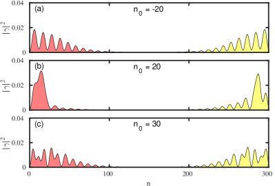
In Sec. III.1, we presented the result of ZMP on the homogeneous wire. In the case of PMP, the behavior of topological ZBP remains unchanged. For a range of values the topological ZBP remains robust (see Fig. 20). The most important difference between the ZMP and the one with the PMP is the MBS’s confinement to the topological region. While for the PMP, the Majorana leaks into the trivial region (see Fig. 21), it is comparatively suppressed for ZMP. The leakage into the ends allow coupling with the lead, restoring the peak width. We find that the peak width exhibits oscillatory dependence on . For example, plotted are the ZBP width for and in Fig. 20, and the corresponding Majorana components in Figs. 21(b-c). For , the Majorana components are away from the lead resulting in small peak width, while for , the leakage of MBS towards the ends of the wire, results in an increase in peak width. While there are certain differences in the signatures corresponding to the two ways of applying the moving protocol, we would like to draw attention to the main signature corresponding to the MBS which remain unaltered for both the protocols i.e. the peak doesn’t move from zero bias throughout the moving protocol.
III.3.2 Inhomogeneous wire
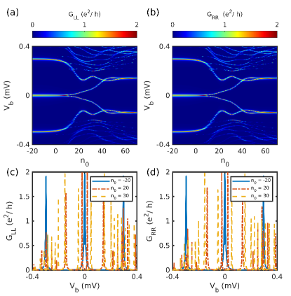
We next consider the NSN system and study the effect of the PMP on the trivial and topological ZBP appearing due to the inhomogenity. As shown in Figs. 22 and 23, the main features regarding the robustness of topological ZBP and the splitting of trivial ZBP remains similar to the ZMP. As for the homogeneous case considered above, oscillations in the topological ZBP width with can be seen. This is again due to the leakage of MBS in the ends of the wire for certain values. For topological zero energy states Majorana components remain separated (see Fig. 24). On the other hand for trivial zero energy states the Majorana components exhibit an increase in overlap, resulting in the splitting of ZBP (see Fig. 25). This result suggests the idea of moving protocol is independent of the method used to put certain parts of the wire in a trivial regime. Both ZMP and PMP can be used to carry out the moving protocol, especially to distinguish topological from trivial ZBP, based on the robustness of the ZBP.
III.4 S′SS′ System
In this last subsection we will study the tunneling conductance and moving protocol results for the S′SS′ system. We’ll utilize this system to highlight some of the shortcomings of the “moving protocol”. Nevertheless it turns out that compare to Zeeman moving protocol the Potential moving protocol is partially immune to some of the shortcomings and can clearly differentiate the topological ZBP signature from the trivial ZBP signature.
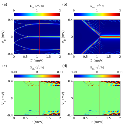
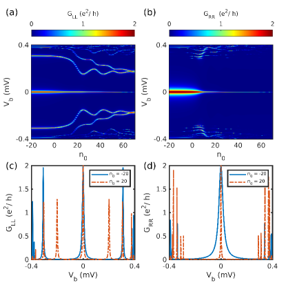
On the either ends of the wire, this system has zero energy states that appear even before the critical Zeeman term (), however, as expected MBS emerges after the critical Zeeman term (see Fig. 26). The zero energy states before the critical zeeman field () are topological in their own right but have partially separable Majorana components, these states prior to the band gap closing are referred to as the quasi-MBS [46, 49]. The tunneling conductance of the system is shown in Fig. 27, where the ZBP corresponding to both the local conductances and the non-local conductance fail to detect the band closing signature. We note that this system’s tunneling conductance signatures are similar to that of the NSN system. Consequently one can not rely only on the tunneling signature to distinguish the trivial and the topological ZBP. Figures 28 and 29 demonstrate how ZMP affects trivial and topological ZBP, respectively. Here, the trivial ZBP peak splitting is only moderately noticeable. The peak splits, but before the split in the peak is pronounced, the peak height drops and disappears. On the other hand for the topological ZBP, the conductance peak is fixed to zero bias for a range of before it too vanishes. We plot the Majorana component for low energy states belonging to the trivial (Fig. 30) and topological (Fig. 31) regimes to determine why this is the case for various values. For trivial zero energy states, the overlap increases with the increase in , leading to a rise in the energy split. Additionally, the states drift away from the lead, weakening the coupling between the lead and the states. As a result, the peak vanishes long before the peak split can be seen clearly. Figure 31 for the topological regime with the MBS demonstrates the presence of the exact shifting of Majorana component away from the lead, which accounts for the decreased peak width and the peak’s disappearance for higher values as depicted in Fig. 29.
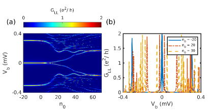
This shortcoming of ZMP is mainly due to the reliance on the local probes to pick the energy split signature. The protocol moves the states away from the lead, which causes the signature to disappear. As we demonstrate in subsection III.3, the PMP is immune to this effect because of the leakage of states towards the ends of the wire, retaining the coupling to the lead. For trivial and topological ZBP, we show the results corresponding to the PMP on the S′SS′ system in Figs. 32 and 33, respectively. Figure 32 clearly illustrates the trivial ZBP splitting during the moving protocol. As shown in Fig. 34, the states leak towards the ends,thereby improving the split visibility. From tunneling conductance plot in Fig. 33 and the analogous Majorana component plot in Fig. 35, it is clear that the resilience of the topological ZBP is also present for this scenario. We want to stress the fact that both moving protocols can induce energy splitting in trivial zero energy states, but as we use local tunneling conductance probe to detect this splitting the PMP is better at capturing the split as well as the robustness in the ZBP.
IV Conclusion
In this article, we have reproduced the tunneling conductance signatures from heterostructures and have verified the inability of local and non-local conductance to distinguish ABS from the MBS. Since both the trivial and non-trivial zero energy states produce a quantized ZBP in local conductance, we focus on the effects of the topological length of the nanowire on the ZBP. We show that by applying the moving protocol, the trivial and topological ZBP behaves differently. As the Majorana component of trivial and topological states are fundamentally different, the protocol affects them differently. For MBS, the Majorana components are entirely separated and localized at the edges of the topological region. The Majorana components move away from the wire’s edges when the protocol is applied, however they remain separated and are therefore pinned at zero energy, causing the peak in local conductance to remain at zero bias throughout the protocol. For trivial zero energy states when the protocol is applied, the overlap between the partially separated Majorana components increases, causing the trivial states to move away from zero energy. As a result, the trivial ZBP splits into two peaks. This effect of moving protocol on topological and trivial ZBP remains the same irrespective of the method of reducing the topological length by putting certain portion of the wire in a trivial regime. We compare the results of ZBP under ZMP and PMP in our numerical simulation. We discuss the shortcoming of the moving protocol in the S′SS′ system, the origin of which is due to the reliance on the local measurements to detect the split in energy. As the states are moved further away from the lead the splitting information is less pronounced in tunneling conductance. However for PMP, the leakage of the states towards the ends preserve the coupling to the leads, making the protocol immune to this vulnerability. Therefore, the PMP which is relatively easier to implement in an experimental setup will be the more suitable protocol for the detection. Our moving protocol combined with existing local tunneling conductance measurement provides a way to differentiate the MBS from the ps-ABS and quasi-MBS. This different response of ZBP under moving protocol clearly distinguishes trivial ZBP from topological ones.
Acknowledgements.
S.G. is grateful to the SERB, Government of India, for the support via the Core Research Grant No. CRG/2020/002731. We also thank J. Carlos Egues and Poliana H. Penteado for the fruitful discussion.Appendix A Calculation of topological quantum number
A.1 Scattering matrix method
To calculate the topological quantum number, we briefly discuss the scattering matrix method here [54]. A scattering matrix characterises a linear relation between the outgoing wave amplitudes and the incoming wave amplitudes at each energy.
| (11) |
The superscript is for amplitudes of the waves moving towards (from) the scatterer and the subscript is for waves on the left (right) of the scatterer. We can express the scattering matrix in terms of transmission and reflection amplitudes in the following form:
| (12) |
Here, represent the 4 4 transmission (reflection) matrices. The transfer matrix relates the wave amplitudes on the right-hand side to the left-hand side of the sample.
| (13) |
From Eq. (11) and Eq. (13), one can express the elements of transfer matrix in terms of the elements of scattering matrix as follows:
| (14) |
Analogous to Eq. (14), we can also decompose the scattering matrix in terms of the elements of the transfer matrix as follows:
| (15) |
The conservation of the probability current also introduces a relationship between the elements of the transfer matrix [57]:
| (16) |
From the definition of transfer matrix it is clear that it obeys the multiplicative composition law,
| (17) |
This composition law for transfer matrices results into a non linear composition of scattering matrices. Using Eq. (14) and Eq. (17), we obtain
| (18) |
This gives the composite -matrix of the system [57]:
| (19) |
The composition law Eq. (19) for scattering matrices is denoted by:
| (20) |
A.2 Topological quantum number
The Hamiltonian in Eq. (1) can be rewritten in the Bogoliubov de-Gennes basis :
| (21) |
Writing the zero-energy Schrödinger’s equation for the BDG Hamiltonian Eq. (21) gives us a recursive relation between two sites in terms of the transfer matrix [54, 58]:
| (22) |
Now, gives the relation between the two nearest-neighbor sites, but it is different from the definition used in Eq. (13). Therefore, we transform to the new basis using a unitary transformation:
| (23) |
In this basis, the transfer matrix now satisfies Eq. (16). As a result, all of the properties of the transfer matrix outlined in section Eq. (A.1) apply to this transfer matrix. Thus, using Eq. (15), we construct the unitary scattering matrix at each site and then using the composition law Eq. (19), we obtain the composite scattering matrix of the N-dot chain:
| (24) |
The topological quantum number TI is given by [59, 60]
| (25) |
where is the subblock of the total scattering matrix Eq. (12) of the chain at Fermi level. The Majorana bound states exist at the endpoints of the chain if . This phase is the topologically nontrivial phase. On the other hand, a value means that the system is in the trivial phase.
Appendix B Tunneling Conductance
The expresion of tunneling conductance in terms of scattering matrix is well known in the literature [61, 62] and is given by
| (26) |
| (27) |
| (28) |
| (29) |
Where is the fermi function at the lead with being L or R. The derivative of fermi function becomes the heavyside fuction at zero kelvin temprature leading to simple equations
| (30) | ||||
| (31) | ||||
| (32) | ||||
| (33) | ||||
We use Green function formalism to calculate the scatering matrixs needed for conductance. The retarded green function for the system conneced to two leads is given by
| (34) |
with as identity matrix and denotes the self energy due to lead. Under the broad band approximation the self energy can be written in terms of level broaderning matrix as . The broaderning matrix is diagonal taking the form . The broadering is treated as a parameter in the numerics to calculate the retarded green function which we fix to for all our calculation. As the BdG hamiltonian is written in Nambu basis the Green fuction has the form
| (35) |
with this perticular form for Green function we could define the scattering matrix elements as
| (36) | ||||||
| (37) | ||||||
| (38) | ||||||
| (39) |
References
- Kitaev [2001] A. Y. Kitaev, Unpaired majorana fermions in quantum wires, 44, 131 (2001).
- Nayak et al. [2008] C. Nayak, S. H. Simon, A. Stern, M. Freedman, and S. Das Sarma, Non-abelian anyons and topological quantum computation, Rev. Mod. Phys. 80, 1083 (2008).
- Alicea [2012] J. Alicea, New directions in the pursuit of majorana fermions in solid state systems, Reports on progress in physics 75, 076501 (2012).
- Sarma et al. [2015a] S. D. Sarma, M. Freedman, and C. Nayak, Majorana zero modes and topological quantum computation, npj Quantum Information 1, 1 (2015a).
- Moore and Read [1991] G. Moore and N. Read, Nonabelions in the fractional quantum hall effect, Nuclear Physics B 360, 362 (1991).
- Rice and Sigrist [1995] T. Rice and M. Sigrist, Sr2ruo4: an electronic analogue of 3he?, Journal of Physics: Condensed Matter 7, L643 (1995).
- Fu and Kane [2008] L. Fu and C. L. Kane, Superconducting proximity effect and majorana fermions at the surface of a topological insulator, Phys. Rev. Lett. 100, 096407 (2008).
- Sau et al. [2010] J. D. Sau, R. M. Lutchyn, S. Tewari, and S. D. Sarma, Generic new platform for topological quantum computation using semiconductor heterostructures, Physical Review Letters 104, 10.1103/PHYSREVLETT.104.040502 (2010).
- Oreg et al. [2010] Y. Oreg, G. Refael, and F. von Oppen, Helical liquids and majorana bound states in quantum wires, Phys. Rev. Lett. 105, 177002 (2010).
- Stanescu et al. [2010] T. D. Stanescu, J. D. Sau, R. M. Lutchyn, and S. D. Sarma, Proximity effect at the superconductor-topological insulator interface, Physical Review B - Condensed Matter and Materials Physics 81, 10.1103/PHYSREVB.81.241310 (2010).
- Albrecht et al. [2016] S. M. Albrecht, A. P. Higginbotham, M. Madsen, F. Kuemmeth, T. S. Jespersen, J. Nygård, P. Krogstrup, and C. Marcus, Exponential protection of zero modes in majorana islands, Nature 531, 206 (2016).
- Churchill et al. [2013] H. O. H. Churchill, V. Fatemi, K. Grove-Rasmussen, M. T. Deng, P. Caroff, H. Q. Xu, and C. M. Marcus, Superconductor-nanowire devices from tunneling to the multichannel regime: Zero-bias oscillations and magnetoconductance crossover, Phys. Rev. B 87, 241401 (2013).
- Das et al. [2012] A. Das, Y. Ronen, Y. Most, Y. Oreg, M. Heiblum, and H. Shtrikman, Zero-bias peaks and splitting in an al–inas nanowire topological superconductor as a signature of majorana fermions, Nature Physics 8, 887 (2012).
- Mourik et al. [2012] V. Mourik, K. Zuo, S. M. Frolov, S. Plissard, E. P. Bakkers, and L. P. Kouwenhoven, Signatures of majorana fermions in hybrid superconductor-semiconductor nanowire devices, Science 336, 1003 (2012).
- Sengupta et al. [2001] K. Sengupta, I. Žutić, H.-J. Kwon, V. M. Yakovenko, and S. Das Sarma, Midgap edge states and pairing symmetry of quasi-one-dimensional organic superconductors, Phys. Rev. B 63, 144531 (2001).
- Setiawan et al. [2017a] F. Setiawan, C.-X. Liu, J. D. Sau, and S. Das Sarma, Electron temperature and tunnel coupling dependence of zero-bias and almost-zero-bias conductance peaks in majorana nanowires, Phys. Rev. B 96, 184520 (2017a).
- Yu et al. [2021] P. Yu, J. Chen, M. Gomanko, G. Badawy, E. P. Bakkers, K. Zuo, V. Mourik, and S. M. Frolov, Non-majorana states yield nearly quantized conductance in proximatized nanowires, Nature Physics 17, 482 (2021).
- Pan and Sarma [2020] H. Pan and S. D. Sarma, Physical mechanisms for zero-bias conductance peaks in majorana nanowires, Physical Review Research 2, 10.1103/PHYSREVRESEARCH.2.013377 (2020).
- Vuik et al. [2019a] A. Vuik, B. Nijholt, A. R. Akhmerov, and M. Wimmer, Reproducing topological properties with quasi-majorana states, SciPost Physics 7, 10.21468/SCIPOSTPHYS.7.5.061/PDF (2019a).
- Pan et al. [2020] H. Pan, W. S. Cole, J. D. Sau, and S. D. Sarma, Generic quantized zero-bias conductance peaks in superconductor-semiconductor hybrid structures, Physical Review B 101, 10.1103/PHYSREVB.101.024506 (2020).
- Chen et al. [2019] J. Chen, B. D. Woods, P. Yu, M. Hocevar, D. Car, S. R. Plissard, E. P. Bakkers, T. D. Stanescu, and S. M. Frolov, Ubiquitous non-majorana zero-bias conductance peaks in nanowire devices, Physical Review Letters 123, 10.1103/PHYSREVLETT.123.107703 (2019).
- Woods et al. [2019] B. D. Woods, J. Chen, S. M. Frolov, and T. D. Stanescu, Zero-energy pinning of topologically trivial bound states in multiband semiconductor-superconductor nanowires, Physical Review B 100, 10.1103/PHYSREVB.100.125407 (2019).
- Vernek et al. [2014] E. Vernek, P. H. Penteado, A. C. Seridonio, and J. C. Egues, Subtle leakage of a majorana mode into a quantum dot, Phys. Rev. B 89, 165314 (2014).
- Grivnin et al. [2019] A. Grivnin, E. Bor, M. Heiblum, Y. Oreg, and H. Shtrikman, Concomitant opening of a bulk-gap with an emerging possible majorana zero mode, Nature Communications 10, 10.1038/S41467-019-09771-0 (2019).
- Moore et al. [2018a] C. Moore, C. Zeng, T. D. Stanescu, and S. Tewari, Quantized zero-bias conductance plateau in semiconductor-superconductor heterostructures without topological majorana zero modes, Physical Review B 94, 10.1103/PHYSREVB.98.155314 (2018a).
- Huang et al. [2018] Y. Huang, H. Pan, C. X. Liu, J. D. Sau, T. D. Stanescu, and S. D. Sarma, Metamorphosis of andreev bound states into majorana bound states in pristine nanowires, Physical Review B 98, 10.1103/PHYSREVB.98.144511 (2018).
- Setiawan et al. [2017b] F. Setiawan, C. X. Liu, J. D. Sau, and S. D. Sarma, Electron temperature and tunnel coupling dependence of zero-bias and almost-zero-bias conductance peaks in majorana nanowires, Physical Review B 96, 10.1103/PHYSREVB.96.184520 (2017b).
- Nichele et al. [2017] F. Nichele, A. C. Drachmann, A. M. Whiticar, E. C. O’Farrell, H. J. Suominen, A. Fornieri, T. Wang, G. C. Gardner, C. Thomas, A. T. Hatke, P. Krogstrup, M. J. Manfra, K. Flensberg, and C. M. Marcus, Scaling of majorana zero-bias conductance peaks, Physical Review Letters 119, 10.1103/PHYSREVLETT.119.136803 (2017).
- Kammhuber et al. [2017] J. Kammhuber, M. C. Cassidy, F. Pei, M. P. Nowak, A. Vuik, O. Gül, D. Car, S. R. Plissard, E. P. Bakkers, M. Wimmer, and L. P. Kouwenhoven, Conductance through a helical state in an indium antimonide nanowire, Nature Communications 8, 10.1038/S41467-017-00315-Y (2017).
- Reeg et al. [2018] C. Reeg, O. Dmytruk, D. Chevallier, D. Loss, and J. Klinovaja, Zero-energy andreev bound states from quantum dots in proximitized rashba nanowires, Phys. Rev. B 98, 245407 (2018).
- Liu et al. [2017a] C. X. Liu, J. D. Sau, T. D. Stanescu, and S. D. Sarma, Andreev bound states versus majorana bound states in quantum dot-nanowire-superconductor hybrid structures: Trivial versus topological zero-bias conductance peaks, Physical Review B 96, 10.1103/PHYSREVB.96.075161 (2017a).
- Cayao et al. [2015] J. Cayao, E. Prada, P. San-Jose, and R. Aguado, Sns junctions in nanowires with spin-orbit coupling: Role of confinement and helicity on the subgap spectrum, Phys. Rev. B 91, 024514 (2015).
- Zhang et al. [2017] H. Zhang, Önder Gül, S. Conesa-Boj, M. P. Nowak, M. Wimmer, K. Zuo, V. Mourik, F. K. D. Vries, J. V. Veen, M. W. D. Moor, J. D. Bommer, D. J. V. Woerkom, D. Car, S. R. Plissard, E. P. Bakkers, M. Quintero-Pérez, M. C. Cassidy, S. Koelling, S. Goswami, K. Watanabe, T. Taniguchi, and L. P. Kouwenhoven, Ballistic superconductivity in semiconductor nanowires, Nature Communications 8, 10.1038/NCOMMS16025 (2017).
- Higginbotham et al. [2015] A. P. Higginbotham, S. M. Albrecht, G. Kiršanskas, W. Chang, F. Kuemmeth, P. Krogstrup, T. S. Jespersen, J. Nygård, K. Flensberg, and C. M. Marcus, Parity lifetime of bound states in a proximitized semiconductor nanowire, Nature Physics 11, 1017 (2015).
- Dmytruk et al. [2020] O. Dmytruk, D. Loss, and J. Klinovaja, Pinning of andreev bound states to zero energy in two-dimensional superconductor- semiconductor rashba heterostructures, Phys. Rev. B 102, 245431 (2020).
- Liu et al. [2017b] C. X. Liu, J. D. Sau, and S. D. Sarma, Role of dissipation in realistic majorana nanowires, Physical Review B 95, 10.1103/PHYSREVB.95.054502 (2017b).
- Prada et al. [2012] E. Prada, P. San-Jose, and R. Aguado, Transport spectroscopy of nanowire junctions with majorana fermions, Phys. Rev. B 86, 180503 (2012).
- Lee et al. [2012] E. J. H. Lee, X. Jiang, R. Aguado, G. Katsaros, C. M. Lieber, and S. De Franceschi, Zero-bias anomaly in a nanowire quantum dot coupled to superconductors, Phys. Rev. Lett. 109, 186802 (2012).
- Prada et al. [2020] E. Prada, P. San-Jose, M. W. de Moor, A. Geresdi, E. J. Lee, J. Klinovaja, D. Loss, J. Nygård, R. Aguado, and L. P. Kouwenhoven, From andreev to majorana bound states in hybrid superconductor–semiconductor nanowires, Nature Reviews Physics 2, 575 (2020).
- San-Jose et al. [2016] P. San-Jose, J. Cayao, E. Prada, and R. Aguado, Majorana bound states from exceptional points in non-topological superconductors, Scientific reports 6, 1 (2016).
- Deng et al. [2016] M. T. Deng, S. Vaitiekenas, E. B. Hansen, J. Danon, M. Leijnse, K. Flensberg, J. Nygård, P. Krogstrup, and C. M. Marcus, Majorana bound state in a coupled quantum-dot hybrid-nanowire system, Science 354, 1557 (2016).
- Song et al. [2022] H. Song, Z. Zhang, D. Pan, D. Liu, Z. Wang, Z. Cao, L. Liu, L. Wen, D. Liao, R. Zhuo, D. E. Liu, R. Shang, J. Zhao, and H. Zhang, Large zero bias peaks and dips in a four-terminal thin inas-al nanowire device, Phys. Rev. Research 4, 033235 (2022).
- Avila et al. [2019] J. Avila, F. Peñaranda, E. Prada, P. San-Jose, and R. Aguado, Non-hermitian topology as a unifying framework for the andreev versus majorana states controversy, Communications Physics 2, 1 (2019).
- Moore et al. [2018b] C. Moore, T. D. Stanescu, and S. Tewari, Two-terminal charge tunneling: Disentangling majorana zero modes from partially separated andreev bound states in semiconductor-superconductor heterostructures, Phys. Rev. B 97, 165302 (2018b).
- Stanescu and Tewari [2019] T. D. Stanescu and S. Tewari, Robust low-energy andreev bound states in semiconductor-superconductor structures: Importance of partial separation of component majorana bound states, Phys. Rev. B 100, 155429 (2019).
- Pan et al. [2021] H. Pan, J. D. Sau, and S. Das Sarma, Three-terminal nonlocal conductance in majorana nanowires: Distinguishing topological and trivial in realistic systems with disorder and inhomogeneous potential, Phys. Rev. B 103, 014513 (2021).
- Hess et al. [2021] R. Hess, H. F. Legg, D. Loss, and J. Klinovaja, Local and nonlocal quantum transport due to andreev bound states in finite rashba nanowires with superconducting and normal sections, Phys. Rev. B 104, 075405 (2021).
- Mishmash et al. [2020] R. V. Mishmash, B. Bauer, F. von Oppen, and J. Alicea, Dephasing and leakage dynamics of noisy majorana-based qubits: Topological versus andreev, Phys. Rev. B 101, 075404 (2020).
- Lai et al. [2021] Y.-H. Lai, S. D. Sarma, and J. D. Sau, Quality factor for zero-bias conductance peaks in majorana nanowire (2021).
- Alicea et al. [2011] J. Alicea, Y. Oreg, G. Refael, F. Von Oppen, and M. Fisher, Non-abelian statistics and topological quantum information processing in 1d wire networks, Nature Physics 7, 412 (2011).
- Sarma et al. [2015b] S. D. Sarma, M. Freedman, and C. Nayak, Majorana zero modes and topological quantum computation, npj Quantum Information 1, 1 (2015b).
- Bauer et al. [2018] B. Bauer, T. Karzig, R. V. Mishmash, A. E. Antipov, and J. Alicea, Dynamics of Majorana-based qubits operated with an array of tunable gates, SciPost Phys. 5, 4 (2018).
- Hu et al. [2015] Y. Hu, Z. Cai, M. A. Baranov, and P. Zoller, Majorana fermions in noisy kitaev wires, Phys. Rev. B 92, 165118 (2015).
- Zhang and Nori [2016] P. Zhang and F. Nori, Majorana bound states in a disordered quantum dot chain, New Journal of Physics 18, 043033 (2016).
- Liu et al. [2017c] C.-X. Liu, J. D. Sau, T. D. Stanescu, and S. Das Sarma, Andreev bound states versus majorana bound states in quantum dot-nanowire-superconductor hybrid structures: Trivial versus topological zero-bias conductance peaks, Phys. Rev. B 96, 075161 (2017c).
- Vuik et al. [2019b] A. Vuik, B. Nijholt, A. Akhmerov, and M. Wimmer, Reproducing topological properties with quasi-majorana states, SciPost Physics 7, 061 (2019b).
- Markos and Soukoulis [2008] P. Markos and C. M. Soukoulis, Wave Propagation: From Electrons to Photonic Crystals and Left-Handed Materials (Princeton University Press, 2008).
- Choy et al. [2011] T.-P. Choy, J. M. Edge, A. R. Akhmerov, and C. W. J. Beenakker, Majorana fermions emerging from magnetic nanoparticles on a superconductor without spin-orbit coupling, Phys. Rev. B 84, 195442 (2011).
- Akhmerov et al. [2011] A. R. Akhmerov, J. P. Dahlhaus, F. Hassler, M. Wimmer, and C. W. J. Beenakker, Quantized conductance at the majorana phase transition in a disordered superconducting wire, Phys. Rev. Lett. 106, 057001 (2011).
- Fulga et al. [2011] I. C. Fulga, F. Hassler, A. R. Akhmerov, and C. W. J. Beenakker, Scattering formula for the topological quantum number of a disordered multimode wire, Phys. Rev. B 83, 155429 (2011).
- Fregoso et al. [2013] B. M. Fregoso, A. M. Lobos, and S. Das Sarma, Electrical detection of topological quantum phase transitions in disordered majorana nanowires, Phys. Rev. B 88, 180507 (2013).
- Lobos and Sarma [2015] A. M. Lobos and S. D. Sarma, Tunneling transport in nsn majorana junctions across the topological quantum phase transition, New Journal of Physics 17, 065010 (2015).