11email: [email protected] 22institutetext: Korea Astronomy and Space Science Institute, 776 Daedeok-daero, Yuseong-gu, Daejeon 34055, South Korea
33institutetext: National Centre for Nuclear Research, ul. L. Pasteura 7, Warsaw 02-093, Poland
33email: [email protected]
Effect of redshift bin mismatch on the cross correlation between the DESI Legacy Imaging Survey and the Planck CMB lensing potential
Abstract
Aims. We study the importance of precise modelling of the photometric redshift error distributions when estimating parameters from cross-correlation measurements. We present a working example of the scattering matrix formalism to correct for the effects of galaxies ending in wrong redshift bins due to their photometric redshift errors.
Methods. We measured the angular galaxy auto-power spectrum and cross-power spectrum in four tomographic bins with the redshift intervals from the cross-correlation of the Planck cosmic microwave background lensing potential and the photometric galaxy catalogue from the Dark Energy Spectroscopic Instrument Legacy Imaging Survey Data Release 8. We estimated the galaxy linear bias and the amplitude of cross correlation using maximum likelihood estimation to put constraints on the parameter.
Results. We show that the modified Lorentzian function used to fit the photometric redshift error distribution performs well only near the peaks of the distribution. We adopt a sum of Gaussians model to capture the broad tails of the error distribution. Our sum of Gaussians model yields values of the cross-correlation amplitude that are smaller than those expected based on the cold dark matter (CDM) model. We compute the parameter after correcting for the redshift bin mismatch of objects following the scattering matrix approach. The parameter becomes consistent with CDM model in the last tomographic bin but shows a tension of in other redshift bins.
Key Words.:
Gravitational lensing: weak – Methods: data analysis – Cosmology: cosmic background radiation1 Introduction
The standard model of cosmology or the cold dark matter (CDM) model, well established based on a vast array of observations, provides us with a comprehensive framework to understand the structure, origin, and evolution of the Universe. The parameters governing the CDM model have been constrained with unparalleled accuracy by precise measurements of the cosmic microwave background (CMB) (Ade et al. 2021; Dutcher et al. 2021; Planck Collaboration et al. 2020b; Aiola et al. 2020; Adachi et al. 2020). However, despite the remarkable success of the CDM model in providing a satisfactory description of the astrophysical and cosmological probes, it cannot explain some of the key ingredients in our understanding of the Universe, namely dark energy (Perlmutter et al. 1999; Riess et al. 1998), dark matter (Trimble, 1987) and inflation (Guth, 1981).
The gravitational lensing of the CMB photons carries information about the growth of structure at redshifts of . Cross correlations between tracers of the large-scale structure and CMB lensing are excellent probes of the evolution of the large-scale gravitational potential and can be used to test the validity of the CDM model. Several works over the past decade have established the importance of such cross-correlation measurements in testing the cosmological model (Saraf et al. 2022; Miyatake et al. 2022; Robertson et al. 2021; Krolewski et al. 2021; Darwish et al. 2021 Abbott et al. 2019; Bianchini & Reichardt 2018; Singh et al. 2017; Bianchini et al. 2016; Bianchini et al. 2015). On the other hand, observations of the probes of large-scale structure, such as weak gravitational lensing and galaxy clustering (Abbott et al. 2022; Philcox & Ivanov 2022; Secco et al. 2022; Amon et al. 2022; Asgari et al. 2021; Skara & Perivolaropoulos 2020; Joudaki et al. 2017; Macaulay et al. 2013) have consistently pointed out a difference in the strength of matter clustering — quantified by the parameter — compared to the conclusions drawn from the CMB-only analysis (Planck Collaboration et al., 2020a).
A large number of studies that implemented the tomographic cross-correlation measurements — by dividing the galaxy samples into narrow redshift bins — reported differences in the values of the , or parameters compared to the values derived from CMB measurements (see Alonso et al. 2023; Wang et al. 2023; Yu et al. 2022; White et al. 2022; Pandey et al. 2022; Chang et al. 2023; Sun et al. 2022; Krolewski et al. 2021; Hang et al. 2021; Marques & Bernui 2020; Peacock & Bilicki 2018; Giannantonio et al. 2016). Other works like Bianchini & Reichardt (2018), Amon et al. (2018), Blake et al. (2016), Giannantonio et al. (2016), and Pullen et al. (2016) find consistent deviations in the values of and statistics when testing the CDM model with different galaxy surveys. Tomographic measurements with upcoming large-scale structure surveys, such as Vera C. Rubin Observatory Legacy Survey of Space and Time (LSST; Ivezić et al. 2019a; LSST Science Collaboration et al. 2009), Euclid (Laureijs et al., 2011), Nancy Grace Roman Space Telescope (Spergel et al., 2013), Dark Energy Spectroscopic Instrument (DESI; Dey et al. 2019), and Spectro-Photometer for the History of the Universe, Epoch of Reionization, and Ices Explorer (SPHEREx; Doré et al. 2014) will help us explore the or tension in unprecedented detail.
The tomographic cross-correlation measurements with photometric galaxy surveys allow us to study the evolution of or to high redshifts but are plagued by photometric redshift errors. The errors on redshift lead to the placement of a fractions of galaxies in wrong redshift bins, referred to here as ‘the redshift bin mismatch’ of galaxies. The effects of redshift bin mismatch on the estimation of parameters have been explored in a few ways (Hang et al. 2021 (hereafter H21); Stölzner et al. 2021; Balaguera-Antolínez et al. 2018). Another attempt to mitigate the bin mismatch of galaxy redshifts and self-calibrate the redshift distributions was proposed by Zhang et al. (2010), who used the scattering matrix formalism. Zhang et al. (2017) proposed an algorithm based on a non-negative matrix factorisation method to compute the scattering matrix and correct the angular power spectra for the redshift scatter. However, the non-negative matrix factorisation method becomes computationally expensive with increasing redshift bins and data points in the angular power spectra. We proposed an alternative method in Shekhar Saraf & Bielewicz (2024) for fast and efficient computations of the scattering matrix validated with Monte Carlo simulations of the LSST survey.
In the present paper, we apply the proof of concept presented in Shekhar Saraf & Bielewicz (2024) to the cross correlation between the Planck CMB lensing potential map and the photometric galaxy catalogues from Data Release 8 of the Dark Energy Spectroscopic Instrument Legacy Imaging Survey prepared by H21. We highlight the importance of precise modelling of the photometric redshift error distributions and quantify the impact of redshift bin mismatch correction on estimation of the parameter. We show that mitigation of redshift bin mismatch is necessary as a second-stage correction in order to obtain unbiased estimates of parameters. We provide a fast and accurate method for redshift bin mismatch correction. We describe the data used in our analysis in section 2 and the modelling of the redshift error distributions in section 3. In section 4, we describe the procedure for estimating the redshift distribution of galaxies taking into account the photometric redshift errors. We expand on the parameter estimation procedure using maximum likelihood estimation in section 5. The mock catalogues used to validate our analysis pipeline are presented in section 6, and various methods for computing the covariance matrix are summarised in section 7. We present the key results from our analysis and comparisons with H21 in section 8. Finally, in section 9, we summarise the findings from our work presented in this paper.
2 Data
2.1 CMB lensing data
We used the lensing potential maps from the third data release (PDR3)111https://pla.esac.esa.int/#cosmology of the Planck collaboration (Planck Collaboration et al., 2020b). PDR3 uses the SMICA DX12 CMB maps to reconstruct the lensing potential from the CMB temperature and polarization data covering of the sky. SMICA (Spectral Matching Independent Component Analysis; Delabrouille et al. 2003) is a foreground component separation method that showed the best performance during the Planck foreground cleaning mock challenge (Planck Collaboration et al., 2014). For our baseline analysis, we used the minimum-variance CMB lensing potential map (hereafter MV map) estimated from the inverse-variance weighting of all lensing estimators based on different correlations of CMB temperature and polarization maps. In addition, Planck PDR3 also provides lensing potential maps estimated only from the CMB temperature measurements (hereafter the TT map) and with deprojection of the Sunyaev-Zeldovich sources (hereafter, the SZ-deproj map). We use the TT and SZ-deproj maps in section 8.2.3 to study the dependence of our results on the choice of the CMB lensing potential map.
The lensing potential was converted to lensing convergence , where is proportional to the two-dimensional Laplacian of . In spherical harmonic space, this relation can be expressed as (Hu, 2000)
| (1) |
The Planck PDR3 package provides spherical harmonics coefficients for the lensing convergence maps at the HEALPix222https://healpix.jpl.nasa.gov/ (Górski et al., 2005) resolution of , which we downgraded to for our analysis. The data package also provides an estimate of the noise power spectrum for the lensing convergence maps along with binary maps masking the regions of the sky not suitable for analysis.
2.2 Legacy survey data
The Dark Energy Spectroscopic Instrument Legacy Imaging Survey (DESI-LIS; Dey et al. 2019) is a combination of three legacy imaging surveys: the Dark Energy Camera Legacy Survey (DECaLS; Blum et al. 2016), the Beijing-Arizona Sky Survey (BASS; Zou et al. 2017) and the Mayall z-band Legacy Survey (MzLS) observed by the Mosaic3 camera (Dey et al., 2016), with the addition of the Dark Energy Survey (DES; The Dark Energy Survey Collaboration 2005). The legacy imaging surveys were motivated by the need to provide targets for the ongoing Dark Energy Spectroscopic Instrument (DESI; DESI Collaboration et al. 2016) survey, and to supplement the Sloan Digital Sky Survey (SDSS; e.g. Abolfathi et al. 2018; Abazajian et al. 2009) photometry data. In our study, we used the galaxy catalogue and photometric redshifts prepared by H21 from the DESI-LIS Data Release 8333http://legacysurvey.org/dr8/, covering a total area of deg2 with sources observed in three optical bands (, , ) and three WISE (Wright et al., 2010) bands: , , and . Due to the shallower effective depth of the and bands, H21 used only the () band, resulting in the following selection criteria being applied to the data:
-
1.
PSF-type objects are excluded which eliminates most stars and quasars.
-
2.
Objects are detected in four bands, i.e. FLUX G|R|Z|W1 ¿ 0.
-
3.
MW TRANSMISSION G|R|Z|W1 are applied to the fluxes for Galactic extinction correction.
-
4.
Magnitude cuts are applied with , , and , where all magnitudes are computed by .
The galaxy density maps are often correlated with systematics uncertainties such as those related to survey depth, stellar density, and observational conditions. H21 generated a completeness map to account for the foreground contaminations at the map pixel level, including masks for bright stars, globular clusters, and incompleteness in optical bands. As DESI-LIS combines data from DECaLS, BASS, MzLS, and DES, there will be additional systematics errors related to the differences in their photometric passbands and limiting magnitudes. The magnitude cuts applied to data significantly reduced the photometric variations and correlations with various foreground contaminants (see section 3.4 of H21 for more details).
H21 used a direct approach to estimate the photometric redshifts of galaxies from observed spectroscopy by assigning a redshift to a given location in multi-colour space. The spectroscopic surveys used to calibrate photometric redshifts included the Galaxy And Mass Assembly (GAMA) survey Data Release 2 (Liske et al., 2015), the SDSS-III Baryon Oscillation Spectroscopic Survey (BOSS) Data Release 12 (Alam et al., 2015), the Extended Baryon Oscillation Spectroscopic Survey (eBOSS) Data Release 16 (Ahumada et al., 2020), the VIMOS Public Extragalactic Redshift Survey (VIPERS) Data Release 2 (Scodeggio et al., 2018), and the DEEP2 (Newman et al., 2013). Two photometric surveys, the Cosmic Evolution Survey (COSMOS) (Ilbert et al., 2009) and the Dark Energy Survey (DES) Y1 redMaGiC (Cawthon et al., 2018), were also included with the spectroscopic surveys for their highly accurate photometric redshifts.
The calibration samples, except DES Y1 redMaGiC, were binned into three-dimensional grids of , , and with a pixel width of about . The ranges of colours used in the three-dimensional grid are , , and . Pixels containing more than five objects from the calibration samples were assigned the mean redshift of these objects. The DES Y1 redMaGiC samples were used to fill in the empty pixels from the initial binning. When calibrating the redshift of galaxies, objects falling in pixels that lack a redshift calibration were excluded. This ensured the selection of objects that occupy the same colour space as the calibration sample. To marginalise digitisation artefacts in the redshift distribution, the assigned photometric redshifts were added with a random top-hat dither of . The resulting redshift calibration led to percent of samples having photometric redshifts of within of their spectroscopic redshifts.
| Redshift Bin | [gal pix-1] | [gal str-1] | median | ||||
|---|---|---|---|---|---|---|---|
| 2.652 | 2.655106 | 0.21 | -0.0010 | 0.0122 | 1.257 | ||
| 2.133 | 2.136106 | 0.38 | 0.0076 | 0.0151 | 1.104 | ||
| 2.487 | 2.490106 | 0.51 | -0.0024 | 0.0155 | 1.476 | ||
| 1.335 | 1.337106 | 0.66 | -0.0042 | 0.0265 | 2.019 |
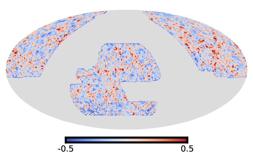
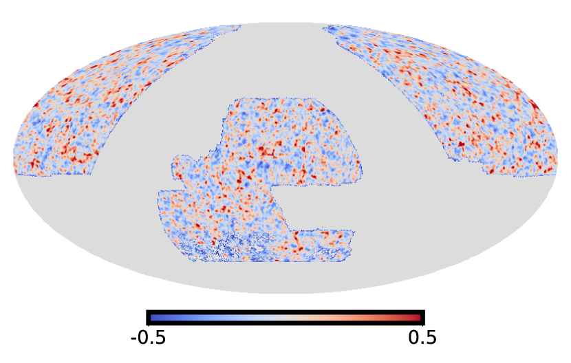
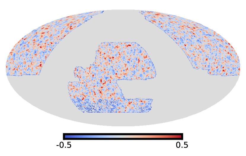
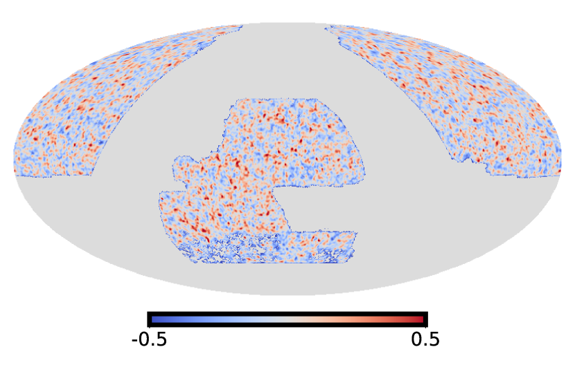
The galaxies were divided into four tomographic bins based on their photometric redshifts with intervals . The galaxy number count maps and the photometric redshift data used in this study are publicly available555https://gitlab.com/qianjunhang/desi-legacy-survey-cross-correlations. A summary of the four tomographic bins including the number of objects and the mean density of objects per pixel and per steradian is given in Table 1. The galaxy over-density maps for every tomographic bin were built at the HEALPix resolution of using the relation
| (2) |
where is the completeness-corrected number of galaxies at angular position and is the mean number of objects. The galaxy over-density maps smoothed with a Gaussian beam of FWHM (for illustrative purposes only) are shown in Fig. 1.
3 Distribution of the photometric redshift error
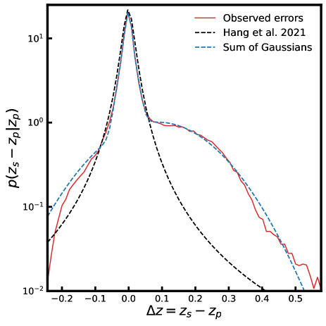
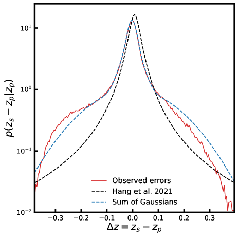
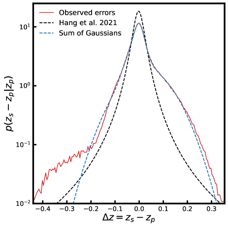
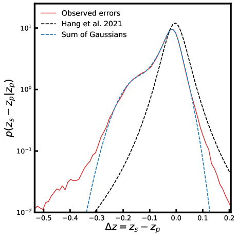
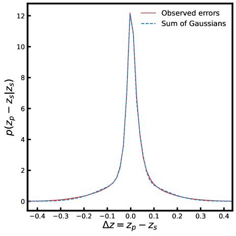
Precise modelling of the distribution of photometric redshift error is required to propagate redshift uncertainties in the estimation of parameters. H21 adopted a modified Lorentzian function (Eq. 3) to model the redshift error distribution of ( spectroscopic; photometric) as a function of , .
| (3) |
where is the normalisation factor and and are the parameters to be constrained for every tomographic bin. The best fit-values of and from H21 are quoted in Table 1.
Fig. 2 shows the photometric error distributions compared to the best-fit modified Lorentzian functions. The modified Lorentzian functions provide a good estimate near the peak of the error distributions but fail to capture the broader tails of the error distribution. We attempted to model the broad wings of the error distributions with a sum of three Gaussians. As shown in Fig. 2, our sum of Gaussians model better captures the tails of the error distributions, at the marginal expense of increasing the number of free parameters in the fitting function. An important point to note is we only seek to fit the broad wings that immediately follow the peak of the error distributions and not the extremities, which is to avoid over-fitting. In section 8.2.1, we detail the impact of modelling the wings of the error distributions on the estimation of parameters.
4 Estimation of the true redshift distribution
An estimate of the true redshift distribution can be computed using either the convolution method or the deconvolution method.
4.1 Convolution method
For the redshift bin, the true redshift distribution was estimated using the observed photometric redshift distribution and the redshift error distribution using the relation
| (4) |
where is the window function defining the boundaries of the redshift bin
| (5) |
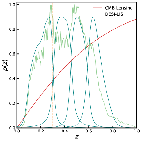
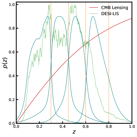
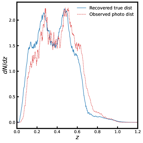
In Fig. 3, we show the galaxy redshift distributions estimated using Eq. (4). The left and the right panels show the redshift distributions estimated with a modified Lorentzian fit of the error distribution and the sum of Gaussians model, respectively. The sum of Gaussians model produces broader tails in the redshift distributions than the modified Lorentzian function, which suggests stronger leakage of objects across redshift bins.
4.2 Deconvolution method
The true redshift distribution in the redshift range can be estimated by using the deconvolution method following the Fourier ratio approach (Shekhar Saraf & Bielewicz, 2024):
| (6) |
where is the observed photometric redshift distribution and is the redshift error distribution built from the spectroscopic calibration sample (section 2.2). We used the deconvolution method to compute the scattering matrix in section 8.2.2.
5 Estimation of parameters
We focused on estimating two parameters, the linear galaxy bias and amplitude of cross correlation , from measurements of the galaxy auto-power spectrum and the cross-power spectrum between CMB lensing and galaxy density, using the maximum likelihood estimation method. The galaxy bias accounts for the fact that galaxies are biased tracers of the underlying total matter distribution. The amplitude of cross correlation is a phenomenological parameter rescaling the amplitude of the cross-power spectrum. The cross correlation amplitude can be used to test the validity of the underlying cosmological model, which in our study is the CDM model (Saraf et al. 2022; Marques & Bernui 2020; Bianchini et al. 2015). The galaxy auto-power spectrum scales as , whereas the cross-power spectrum depends on the product of the parameters and induces a degeneracy in the estimation of parameters. We break this degeneracy using a joint likelihood function of the form
| (7) |
where is the number of data points and is the measured joint power spectrum, . Also, is the joint theoretical power spectrum template defined as , and the covariance matrix is given as
| (8) |
In section 7, we outline different ways to estimate the covariance matrix .
We employed the publicly available EMCEE (Foreman-Mackey et al., 2013) package to effectively sample the parameter space, and estimated the galaxy bias and the cross-correlation amplitude . We used flat priors for the parameters with and . The other cosmological parameters entering the likelihood estimation through theoretical power spectrum templates were set to their constant values for the fiducial background cosmology described in Planck Collaboration et al. (2020a) (i.e. the flat CDM cosmology with the best-fit Planck + WP + highL + lensing parameters, where WP stands for the WMAP polarisation data at low multipoles, highL is the high-resolution CMB data from the Atacama Cosmology Telescope (ACT) and the South Pole Telescope (SPT), and lensing refers to the inclusion of Planck CMB lensing data in the parameter likelihood).
6 Mock catalogues
To gain insight into how the observed redshift errors impact the estimation of parameters, we created mock catalogues following the same approach to simulations as in our previous paper, Shekhar Saraf & Bielewicz (2024). We used the publicly available code FLASK (Xavier et al., 2016) and created Monte Carlo simulations of correlated log-normal galaxy density field with observed DESI-LIS physical properties (quoted in Table 1) and Planck CMB lensing convergence field. The photometric redshifts were generated from the observed photometric redshift error distributions . We divided the simulated galaxy catalogue into five redshift bins with intervals of . We introduced an additional redshift bin of in simulations to account for the scatter of galaxies outside the redshift range considered in the analysis, which is . The theoretical power spectra for galaxy auto-correlation, CMB convergence auto-correlation and their cross correlation were computed from the Limber approximation (Limber, 1953) using the relation
| (9) |
where , convergence and galaxy over-density. Here, is the comoving distance, and is the comoving distance to the surface of the last scattering at redshift . Also, is the matter power spectrum which is generated using the publicly available cosmology code CAMB666https://camb.info/(Lewis et al., 2000) with the HALOFIT prescription to take into account the non-linear distribution of matter. and are lensing and galaxy kernels given by
| (10) | ||||
| (11) |
We used a redshift-dependent galaxy bias (Solarz et al. 2015; Moscardini et al. 1998; Fry 1996)
| (12) |
where and is the normalised growth function
| (13) |
where is the growth index for the general relativity (Linder, 2005).
We used the CMB convergence noise power spectrum from Planck PDR3 to add noise to the simulated CMB lensing convergence maps. To introduce noise in the galaxy density field, we let FLASK Poisson sample the number of galaxies in mock catalogues.
7 Covariance matrix
In this section, we explore three different ways to estimate the covariance matrix (Eq. 8).
7.1 Analytical covariance matrix
The analytical covariance matrix between Gaussian fields and estimated using Saraf et al. (2022) is given by
| (14) |
where , is the fraction of sky common to fields and , and is the composite quantity that acts as a weight when taking into account different observed sky areas for different fields. The analytical covariance confers the advantage that sampling fluctuations, known as cosmic variance, are already included in the matrix. It can also be computationally fast to estimate using arbitrary theoretical power spectra.
7.2 Sample covariance from mock realisations
From the simulations of the galaxy density and CMB convergence fields (as described in section 6), one can compute an unbiased estimator of the covariance matrix as
| (15) |
where is the average power spectrum from Monte Carlo simulations, represents the simulated power spectrum estimate, and is the number of simulations.
7.3 Jackknife method
The advantage of the jackknife method is that it is independent of any assumptions regarding the cosmological model. As this method uses data for the estimation of the covariance matrix, it also naturally takes into account the different survey selection effects and any unforeseen systematic errors. However, the jackknife method assumes that the observed data are an accurate representation of the distribution of measurements and is inherently blind to cosmic variance.
To apply the jackknife method, we followed the delete-one approach and made disjoint partitions of the DESI-LIS survey footprint. We then computed the angular power spectra by omitting one subsample at a time. If we use to denote the angular power spectrum computed by removing the subsample, the covariance matrix can be estimated as (Norberg et al., 2009)
| (16) |
where is the mean power spectrum over all subsamples.
7.4 From H21
H21 estimated the covariance matrix from the errors computed directly from the observed data. The observed angular power spectra were binned into groups with multipole bin width
| (17) |
The errors on the binned data points were computed as
| (18) |
The diagonal covariance matrix is then given by .
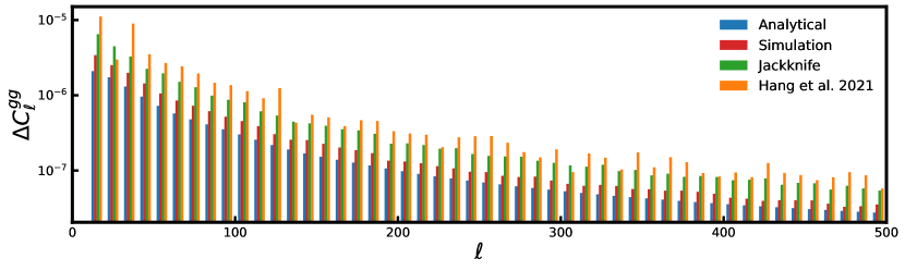
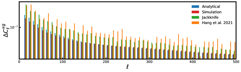
In Fig. 4 we show the power spectrum errors estimated as the square root of the diagonal elements of the covariance matrix from different methods for the redshift slice . We find that the internal methods, namely the jackknife method and the covariance matrix from H21 showed larger contributions to the diagonal elements of the covariance matrix. The analytical covariance and the sample covariance from mock realisations are underestimated, suggesting that the nuances of the data are not captured by these methods. We find similar results for other redshift bins and chose to use the covariance matrix from H21 for the estimation of parameters.
8 Results: DESI-LIS Planck
We followed the analysis choice of H21 and binned the measured galaxy auto-power spectra and cross-power spectra between the DESI-LIS photometric galaxy catalogue and the Planck minimum-variance CMB lensing potential map with a bin width of in the multipole range . In this section, we present our estimates of galaxy bias and cross-correlation amplitude, taking into account the effects of redshift bin mismatch of objects across tomographic bins.
8.1 Mock catalogues
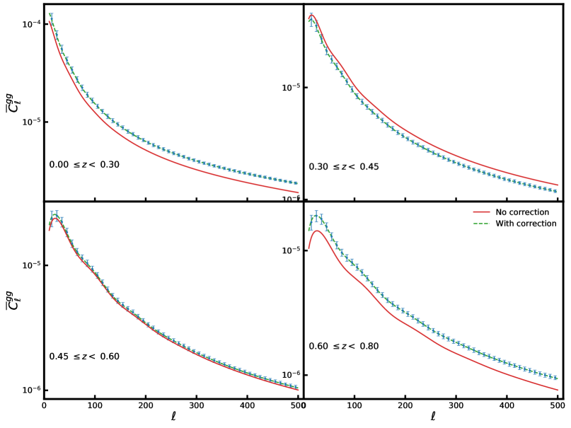
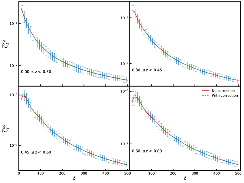
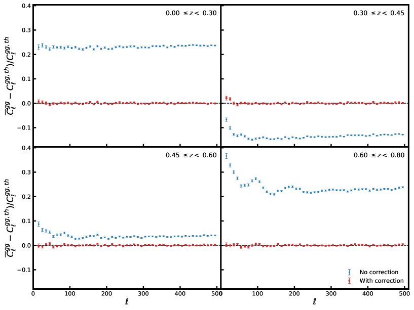
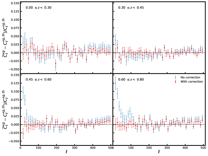
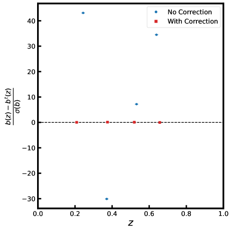
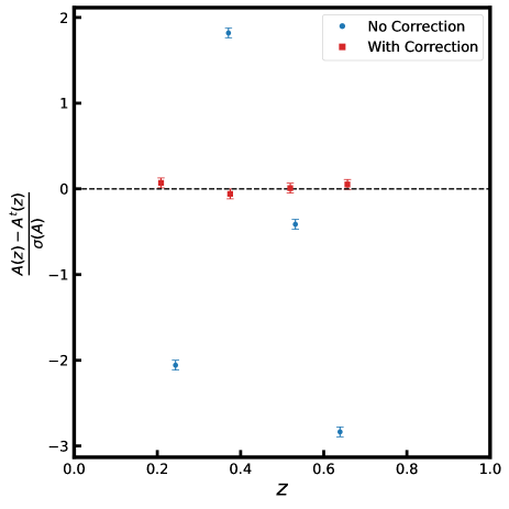
In section 6, we describe the mock catalogues prepared using the code FLASK with the DESI-LIS observed photometric redshift errors. We validate our pipeline and estimate the impact of the redshift bin mismatch of DESI-LIS galaxies in this section. We follow the procedure from Shekhar Saraf & Bielewicz (2024) to estimate galaxy bias and cross-correlation amplitude from simulated photometric datasets. In Fig. 5, we show the deviations of the estimated values of the galaxy linear bias (left panel) and the amplitude of cross-correlation (right panel) from their fiducial values used in simulations in terms of standard deviations. The values of parameters are computed from the average power spectra of simulations before (blue circles) and after (red squares) accounting for the redshift bin mismatch of objects. The average power spectra and relative differences between the averages and best-fit theoretical spectra are shown in Appendix A (Figs. 16 and 17, respectively). Before leakage correction, the galaxy bias was higher, with deviations in three out of four tomographic bins. The second redshift bin gives a lower estimate of the galaxy bias. Such large deviations in terms of errors are a consequence of small uncertainties on the galaxy bias constrained from the galaxy auto-power spectrum. We find the amplitude of cross-correlation to be smaller than unity by in three redshift bins, and higher by in the second redshift bin. The estimated parameters closely follow their expected values after accounting for the leakage across redshift bins.
8.2 DESI-LIS Planck
In this section, we present the measurements of angular power spectra and parameter estimates from cross correlation of the DESI-LIS photometric galaxy catalogue with Planck CMB lensing potential maps.
8.2.1 Before leakage correction
H21 estimated the galaxy bias directly from the measured galaxy-auto power spectrum, , across all tomographic bins by adopting a two-parameter bias model for the linear and non-linear regimes:
| (19) |
where the linear power spectrum and the non-linear correction are computed using CAMB. The galaxy bias for individual redshift bins is given by
| (20) |
with
| (21) |
where are the errors on the galaxy auto-power spectra (Eq. 18). The choice of a two-parameter bias model is motivated by the fact that the galaxy auto-power spectra cannot be fit well by a constant bias beyond (see section 4.1.1 of H21).
To account for the photometric redshift uncertainties, H21 extended the set of free parameters to {}, where and are nuisance parameters that define the modified Lorentzian model for the error distribution in the redshift bin. The constraints on the nuisance parameters were derived from the galaxy–galaxy cross power spectra between tomographic bins. The cross-correlation amplitudes for redshift bins were estimated from the galaxy-CMB lensing cross-power spectrum (with an estimate of galaxy linear bias from Eq. 20). The H21 best-fit values of are quoted in Table 1 and the values of galaxy linear bias — to which we compare estimates of the galaxy bias for our model — and cross correlation amplitude are mentioned in Table 2. We find our estimates of the cross-correlation amplitude to be in tension with respect to the CDM expectations at .
In Shekhar Saraf & Bielewicz (2024), we showed that estimations of galaxy bias from the galaxy auto-power spectrum alone in tomographic analyses produced biased results due to redshift bin mismatch of objects, even with a precise model of the photometric redshift error distribution. We aim to correct the scatter of objects across redshift bins through the scattering matrix formalism. For the DESI-LIS datasets, we estimated the effective maximum wave number (or ), where we expect the non-linear corrections to be mild. Thus, instead of the H21 two-bias model, we used a single-parameter redshift-dependent model of galaxy bias, , and a non-linear theoretical power spectrum computed using CAMB with the HALOFIT prescription.
Before correcting the redshift bin mismatch, we compared our estimates of the galaxy linear bias and cross-correlation amplitude to the estimates from H21 in Table 2. For the modified Lorentzian error distribution, we find good agreement between the galaxy bias estimates, whereas the cross-correlation amplitudes differ by in all redshift bins. We find the amplitude to be consistent with the CDM model in the last two tomographic bins and a deviation in the other two redshift bins. It is worth noting that, although we estimated the covariance matrix in the same way as H21 in this analysis, we obtain smaller errors in galaxy bias.
We also quote in Table 2 the best-fit values of parameters and adopting the sum of Gaussian model for the photometric redshift error distribution. We consistently estimate higher values of galaxy bias and lower values for the amplitude of the cross-correlation across all redshift bins compared to the modified Lorentzian fit, except for the first bin where the amplitude is found to be higher than the modified Lorentzian fit by . The tension in the amplitude with respect to the CDM model rises to with the sum of Gaussians approach, with the strongest deviation observed in the second redshift bin.
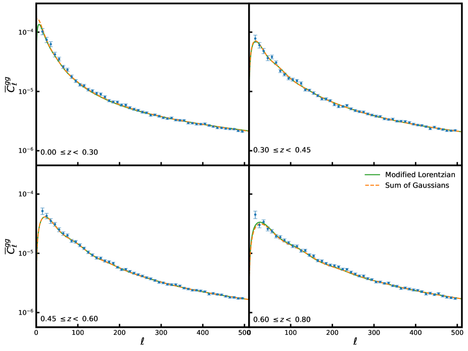
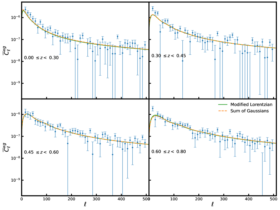
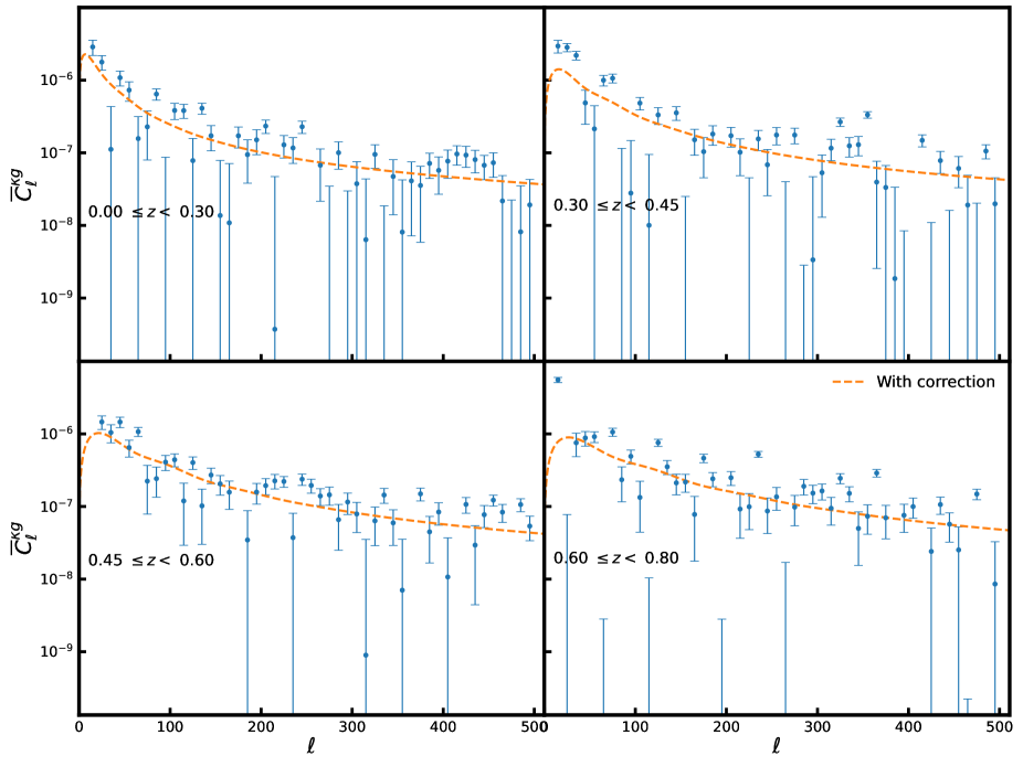
We computed the reduced values for the best-fit theoretical power spectrum to the measured angular cross-power spectrum with degrees of freedom to establish the goodness of fit with modified Lorentzian and the sum of Gaussian models. The values show that both error distribution models can be used for the analysis of the data. Figures 6 and 7 show the measured galaxy auto-power spectra and cross-power spectra for the four tomographic bins, with the best-fit theoretical power spectra computed using modified Lorentzian (solid green line) and the sum of Gaussians (dashed orange line) fit to the error distributions. As the sum of Gaussians model better captures the peculiarities of the error distributions (as shown in Fig. 2), we treat the parameters estimated under this model as our baseline results.
| Bin | From Hang et al. | This work | ||||||
|---|---|---|---|---|---|---|---|---|
| Modified Lorentzian | Sum of Gaussians | |||||||
8.2.2 With leakage correction
As mentioned above, the parameters estimated in a tomographic cross-correlation study will be biased unless the power spectra are corrected for the redshift bin mismatch of objects. In Shekhar Saraf & Bielewicz (2024), we proposed a fast and efficient scattering matrix method to correct the mismatch of objects. Computation of the scattering matrix requires estimation of the true redshift distribution. We use the deconvolution method described in section 4.2 to estimate the true redshift distribution from the observed photometric redshift distribution and a model of the error distribution . In Fig. 8 we show the sum of Gaussians fit to and the true redshift distribution recovered using the deconvolution method.
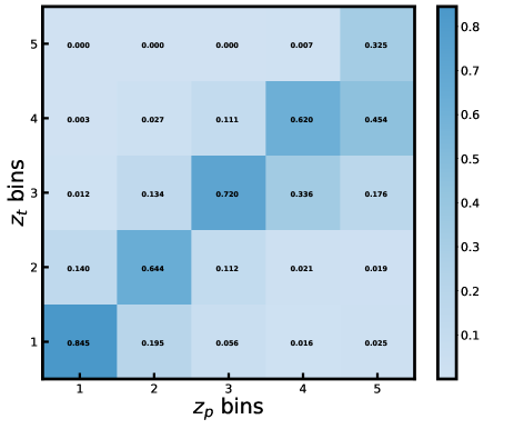
Due to photometric redshift errors, some galaxies from will be wrongly placed at higher redshifts. To account for this loss of objects, we extended the estimation of the auto- and cross-power spectra as well as the scattering matrix for the tomographic bin , following the procedure outlined in section 2. In Fig. 9, we compare the scattering matrix computed for the DESI-LIS photometric catalogue with the mean true scattering matrix estimated from Monte Carlo simulations described in section 6. The similarities in the scattering matrices from data and simulations are expected given that we used the observed photometric error distribution in our simulations. On these grounds, we expect the scattering matrix estimated from the data to be robust in correcting the power spectra.

The leakage-corrected galaxy auto- and cross-power spectra and were computed from the matrix relations (Shekhar Saraf & Bielewicz, 2024)
| (22) | ||||
| (23) |
where and are the scattering matrix and its transpose, and and are the power spectra estimated from the DESI-LIS catalogue and its cross correlation with the Planck CMB lensing map (presented in section 8.2.1). To compute the parameters from the estimates of the true power spectra using the maximum likelihood estimation method, we used the power spectrum template for each tomographic bin given by
| (24) | ||||
| (25) |
where and are free parameters and is given by
| (26) |
where is the true redshift distribution computed using the deconvolution method and is window function given by Eq. (5).
| Bin | From Hang et al. | This work | ||||||
|---|---|---|---|---|---|---|---|---|
| Before correction | After correction | |||||||
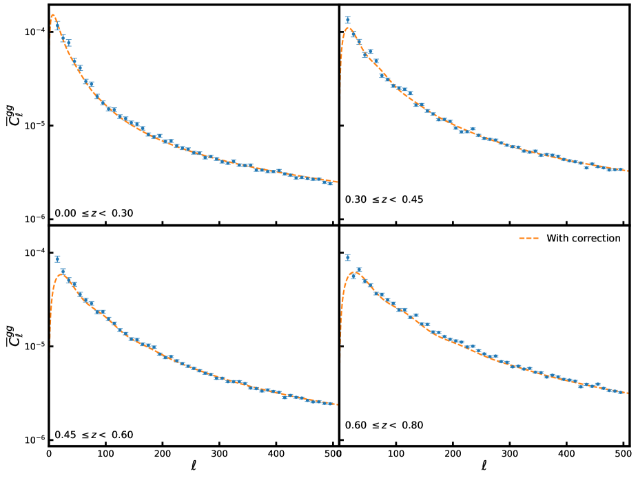
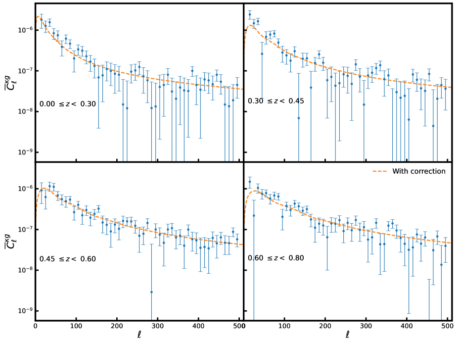
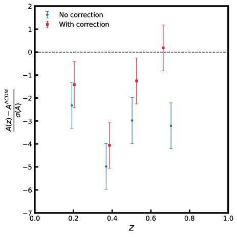
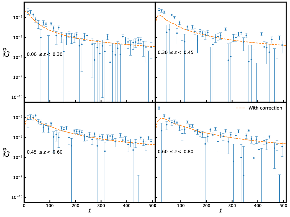
In Figures 10 and 11, we show the galaxy auto-power spectra and cross-power spectra for the four tomographic bins corrected for the redshift bin mismatch of galaxies and the corresponding best-fit theoretical power spectra. In Table 3, we compare the parameters and computed before and after leakage correction for our baseline results using the sum of Gaussians fit to the redshift error distributions. The cross-correlation amplitude is notably higher in all tomographic bins after correction for redshift bin mismatch and becomes consistent with unity in the last tomographic bin. The tension in the amplitude remains at in the second redshift bin, but reduces to in other redshift bins. We note that the amplitude of cross correlation is consistent with the estimates of H21, except for the last redshift bin where we quote a higher value of by . The behaviour in the last bin can be understood as an effect of including the objects scattered outside the redshift range , which were not considered by H21. The galaxy bias, however, differs significantly between our estimates. We find lower values of the galaxy bias after correcting our baseline results with the scattering matrix formalism. We report values of galaxy bias that are slightly different from those of H21 which could result from our different assumptions in the model for galaxy bias evolution. As the amplitude of cross correlation is consistent, we believe that the need for a two-parameter bias model (Eq. 20) may also have been created as a result of the redshift bin mismatch of objects. In Fig. 12, we present the deviations of the estimated amplitude of cross correlation from its expected value () in terms of the standard deviation of the amplitude. By countering the impact of redshift bin mismatch, we reduce the tension in amplitude from to , with complete agreement within errors for the last tomographic bin.
We note the peculiar behaviour of the second redshift bin — correction with scattering matrix does not affect the amplitude of cross correlation whereas our simulations predict an increase in the galaxy bias (or a corresponding reduction in the amplitude) after correction of the redshift bin mismatch (see Fig. 5). A possible explanation for the different behaviour can be found in section 3.2 of H21 where the authors mention that, for their redshift calibration, a small proportion of objects with spectroscopic redshifts of were assigned photometric redshifts of . This systematic in the H21 redshift calibration will impact the photometric redshift error distribution and we might underestimate the scatter of objects from the second redshift bin.
Having estimates of the galaxy bias from four redshift bins we can compute the galaxy bias at redshift zero, , from our model of galaxy bias . We find without and with correction for redshift bin mismatch, respectively. Accounting for the scatter of objects between redshift bins leads to a significantly lower value of and will result in different inferences about the relation between the dark matter and luminous matter.
8.2.3 Using different CMB lensing potential maps
Although accounting for leakage reduces the deviations observed on the amplitude of cross correlation for our baseline analysis, there remains a tension concerning the prediction of the standard cosmological model. There are several galaxy survey systematic errors, such as catastrophic errors, photometric calibration errors, and magnification, that can affect the estimation of power spectra in a cross correlation analysis. We have not considered these systematic errors with DESI-LIS datasets, because the goal of this study is to convey the importance of redshift mismatch correction in the estimation of parameters. However, one of the important conclusions from Saraf et al. (2022) was that different CMB lensing convergence maps produce significantly different values of the cross-correlation amplitude parameter. Hence, in this section, we compared estimates of galaxy bias and cross-correlation amplitude obtained from the SZ-deproj and TT CMB lensing convergence maps.
| Bin | MV | SZ-deproj | TT | ||||||
|---|---|---|---|---|---|---|---|---|---|
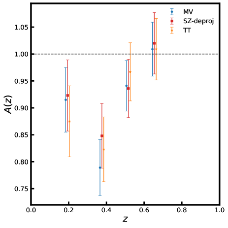
In Table 4, we compare the best-fit values of parameters and estimated for cross correlation of DESI-LIS tomographic bins with MV, SZ-deproj, and TT CMB lensing convergence maps after leakage correction. As we can see from the right panel of Fig. 12, the amplitude estimated with the SZ-deproj map is found to be in agreement with the MV map, except in the second redshift bin, where the SZ-deproj map prefers a higher value than the MV map. The TT map, on the other hand, is consistent with the MV map overall, while alleviating the tension on the cross-correlation amplitude for the third and fourth tomographic bins. Figures 13 and 14 show the redshift-bin-mismatch-corrected cross-power spectra for the four tomographic bins with SZ-deproj and TT maps, respectively.
8.3 Estimation of the parameter
The amplitude of cross-correlation can be translated to the parameter using the relation (Peacock & Bilicki, 2018)
| (27) |
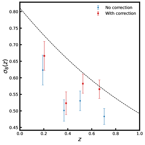
where is the value of the parameter at redshift . In the left panel of Fig. 15, we show the impact of redshift bin mismatch on the parameter estimated from our baseline analysis for the cross-correlation measurements between the DESI-LIS photometric galaxy catalogue and the Planck MV CMB lensing potential. The dashed black line is the redshift evolution of for our fiducial cosmology. The parameter, after correcting for the redshift bin mismatch of objects, agrees better with the predictions of the CDM model overall, becoming fully consistent in the last tomographic bin. However, there remains a discrepancy in the first redshift bin, a difference for the second redshift bin, and a discrepancy for the third redshift bin in the parameter compared to the CDM model. The observed tension in the parameter with respect to the standard cosmological model is consistent with other measurements (Nakoneczny et al. 2024; Chang et al. 2023; White et al. 2022; Sun et al. 2022; Krolewski et al. 2021).
A possible reason for this discrepancy with the DESI-LIS dataset could be systematic uncertainty in the redshift calibration performed by H21, as already mentioned in section 8.2.2. In the estimation of photometric redshifts by H21, a proportion of objects with spectroscopic redshifts between were assigned photometric redshifts between . This systematic error will significantly impact the bin mismatch correction based on the scattering matrix and estimation of the parameter. In addition, there can be residual photometric calibration errors across the three legacy imaging surveys (DECaLS, BASS, MzLS), which can alter the measured angular power spectrum. However, the goal of this study is to present the scattering matrix approach for the correction of redshift bin mismatch in observational data. A detailed analysis of other systematic uncertainties and their impact on the tension is outside the scope of this work and we reserve such analyses for future studies.
If these systematic errors were not able to explain the observed offsets in the parameter, then we could conclude that there is a mild tension with the CDM model. A wide range of scenarios are being considered in the literature to explain the tension in cosmology, such as the impact of redshift space distortions (Macaulay et al., 2013), a redshift dependence of the parameter (Adil et al., 2024), or modifications to the standard cosmological model (see Abdalla et al. 2022 for a comprehensive review).
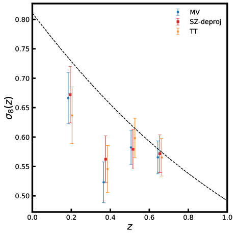
In the right panel of Fig. 15, we compare the parameter computed from the cross-correlation measurements with MV, SZ-deproj, and TT CMB lensing maps. The estimates of parameters from different CMB lensing maps are consistent with each other. In Table 5, we compare values of galaxy bias and for the four DESI-LIS tomographic bins obtained before and after correction for redshift bin mismatch of objects.
| leakage | |||||||||
|---|---|---|---|---|---|---|---|---|---|
| correction | () | () | () | () | |||||
| H21 | no | ||||||||
| This work | no | ||||||||
| yes | |||||||||
9 Summary
We performed a tomographic cross-correlation analysis between the minimum-variance CMB lensing convergence map from Planck Collaboration et al. (2020b) and photometric galaxy catalogues from the Data Release 8 of Dark Energy Spectroscopic Instrument Legacy Imaging Survey prepared by H21. We divided the galaxy density field into four redshift slices covering , with a photometric redshift precision of in the range .
H21 used a modified Lorentzian function to approximate the photometric redshift error distribution. Here, we show that the modified Lorentzian function performs well only near the peaks of the error distribution but fails to capture the tails of the error distribution. Although the number of objects in the tails of the error distribution will be smaller than in the peak, we show that broad tails significantly affect the estimation of parameters by adopting a better fitted sum of Gaussians model for the redshift error distributions. We find that our ‘sum of Gaussians’ model gives smaller values for the cross-correlation amplitude and significantly higher estimates of the galaxy linear bias than H21. As the sum of Gaussians model better captures the peculiarities of the error distributions, we treat the parameters estimated under this model as our baseline results.
We implemented the scattering matrix formalism presented in Shekhar Saraf & Bielewicz (2024) to correct for the scatter of objects across redshift bins causing biased estimation of parameters. For our baseline analysis with the sum of Gaussians fit to the redshift error distributions, we find a higher values of the amplitude of cross correlation from three out of four tomographic bins after correction for leakage, whereas no significant change was observed in the second redshift bin. This may be caused by a small proportion of objects with redshifts between , that have assigned photometric redshifts between , as mentioned by H21 in section 3.2 of their paper. Due to this systematic error in the redshift calibration, we may underestimate the scattering matrix elements for the second redshift bin. Our estimates of cross-correlation amplitude are consistent with the CDM expectations, except for the last redshift bin where we get a value that is higher by , making it completely consistent with CDM expectations. The difference in the last bin could be the result of taking into account objects with redshift of higher than 0.8 in our analysis, which were not considered by H21. However, the galaxy bias differs significantly from H21, primarily due to the different models of galaxy bias.
As shown by Saraf et al. (2022), different CMB lensing maps produce significantly different cross-correlation amplitudes. To test this dependence, we estimated galaxy linear bias and cross-correlation amplitude using Sunyaev-Zeldovich deprojected (SZ-deproj) and temperature-only (TT) reconstructions of the CMB lensing convergence maps. We found the results from SZ-deproj and TT maps to be consistent with the MV map overall. The SZ-deproj map yields an higher value for cross-correlation amplitude in the second tomographic bin and the TT map completely resolves the deviation on the amplitude with respect to the CDM model for the last two tomographic bins, but with poorer values. Finally, we estimated the impact of the redshift mismatch correction on the parameter. We find that the corrected power spectra yields estimates that are consistent with the standard cosmological model for the fourth bin, smaller by around for the first and third bins, and smaller by for the second bin.
In this study, we demonstrate the importance of precise modelling of the photometric redshift error distributions when estimating parameters such as from cross-correlation measurements and present a working example of scattering matrix formalism to correct for the redshift bin mismatch of objects in tomographic cross-correlation analysis. The tension is one of the pressing challenges of modern cosmology. Upcoming large-scale structure surveys such as Vera C. Rubin Observatory Legacy Survey of Space and Time (Ivezić et al. 2019b; LSST Science Collaboration et al. 2009), are expected to have smaller redshift errors. This will enable us to put tighter constraints on the tension with future tomographic cross-correlation measurements. However, the statistical errors of these surveys will also be small and the net outcome of the bin mismatch systematic error will depend on the interplay between redshift errors and survey statistical errors. From the results for simulations of the LSST survey presented in our previous publication Shekhar Saraf & Bielewicz (2024), we can expect the redshift bin mismatch to remain a significant systematic error even for future photometric datasets. Here we show that the method developed in Shekhar Saraf & Bielewicz (2024) based on the use of the scattering matrix offers a robust way to mitigate bin mismatch, which should enable unbiased inference of cosmological parameters from future tomographic measurements.
Acknowledgements.
We thank the anonymous referee whose comments helped to increase the quality of the manuscript. We thank Qianjun Hang for providing DESI-Legacy Imaging Survey datasets. CSS thanks Maciej Bilicki for providing feedback on the data analysis in the paper. The authors thank Agnieszka Pollo for various discussion on the content of this paper. The authors acknowledge the use of CAMB, HEALPix, EMCEE and FLASK software packages. The work has been supported by the Polish Ministry of Science and Higher Education grant DIR/WK/2018/12 and is based on observations obtained with Planck (http://www.esa.int/Planck), an ESA science mission with instruments and contributions directly funded by ESA Member States, NASA, and Canada.References
- Abazajian et al. (2009) Abazajian, K. N., Adelman-McCarthy, J. K., Agüeros, M. A., et al. 2009, ApJS, 182, 543
- Abbott et al. (2019) Abbott, T. M. C., Abdalla, F. B., Alarcon, A., et al. 2019, Phys. Rev. D, 100, 023541
- Abbott et al. (2022) Abbott, T. M. C., Aguena, M., Alarcon, A., et al. 2022, Phys. Rev. D, 105, 023520
- Abdalla et al. (2022) Abdalla, E., Abellán, G. F., Aboubrahim, A., et al. 2022, Journal of High Energy Astrophysics, 34, 49
- Abolfathi et al. (2018) Abolfathi, B., Aguado, D. S., Aguilar, G., et al. 2018, ApJS, 235, 42
- Adachi et al. (2020) Adachi, S., Aguilar Faúndez, M. A. O., Arnold, K., et al. 2020, ApJ, 904, 65
- Ade et al. (2021) Ade, P. A. R., Ahmed, Z., Amiri, M., et al. 2021, Phys. Rev. Lett., 127, 151301
- Adil et al. (2024) Adil, S. A., Akarsu, Ö., Malekjani, M., et al. 2024, MNRAS, 528, L20
- Ahumada et al. (2020) Ahumada, R., Allende Prieto, C., Almeida, A., et al. 2020, ApJS, 249, 3
- Aiola et al. (2020) Aiola, S., Calabrese, E., Maurin, L., et al. 2020, J. Cosmology Astropart. Phys., 2020, 047
- Alam et al. (2015) Alam, S., Albareti, F. D., Allende Prieto, C., et al. 2015, ApJS, 219, 12
- Alonso et al. (2023) Alonso, D., Fabbian, G., Storey-Fisher, K., et al. 2023, J. Cosmology Astropart. Phys., 2023, 043
- Amon et al. (2018) Amon, A., Blake, C., Heymans, C., et al. 2018, MNRAS, 479, 3422
- Amon et al. (2022) Amon, A., Gruen, D., Troxel, M. A., et al. 2022, Phys. Rev. D, 105, 023514
- Asgari et al. (2021) Asgari, M., Lin, C.-A., Joachimi, B., et al. 2021, A&A, 645, A104
- Balaguera-Antolínez et al. (2018) Balaguera-Antolínez, A., Bilicki, M., Branchini, E., & Postiglione, A. 2018, MNRAS, 476, 1050
- Bianchini et al. (2015) Bianchini, F., Bielewicz, P., Lapi, A., et al. 2015, ApJ, 802, 64
- Bianchini et al. (2016) Bianchini, F., Lapi, A., Calabrese, M., et al. 2016, ApJ, 825, 24
- Bianchini & Reichardt (2018) Bianchini, F. & Reichardt, C. L. 2018, ApJ, 862, 81
- Blake et al. (2016) Blake, C., Joudaki, S., Heymans, C., et al. 2016, MNRAS, 456, 2806
- Blum et al. (2016) Blum, R. D., Burleigh, K., Dey, A., et al. 2016, in American Astronomical Society Meeting Abstracts, Vol. 228, American Astronomical Society Meeting Abstracts #228, 317.01
- Cawthon et al. (2018) Cawthon, R., Davis, C., Gatti, M., et al. 2018, MNRAS, 481, 2427
- Chang et al. (2023) Chang, C., Omori, Y., Baxter, E. J., et al. 2023, Phys. Rev. D, 107, 023530
- Darwish et al. (2021) Darwish, O., Madhavacheril, M. S., Sherwin, B. D., et al. 2021, MNRAS, 500, 2250
- Delabrouille et al. (2003) Delabrouille, J., Cardoso, J. F., & Patanchon, G. 2003, MNRAS, 346, 1089
- DESI Collaboration et al. (2016) DESI Collaboration, Aghamousa, A., Aguilar, J., et al. 2016, arXiv e-prints, arXiv:1611.00037
- Dey et al. (2016) Dey, A., Rabinowitz, D., Karcher, A., et al. 2016, in Ground-based and Airborne Instrumentation for Astronomy VI, ed. C. J. Evans, L. Simard, & H. Takami, Vol. 9908, International Society for Optics and Photonics (SPIE), 99082C
- Dey et al. (2019) Dey, A., Schlegel, D. J., Lang, D., et al. 2019, AJ, 157, 168
- Doré et al. (2014) Doré, O., Bock, J., Ashby, M., et al. 2014, arXiv e-prints, arXiv:1412.4872
- Dutcher et al. (2021) Dutcher, D., Balkenhol, L., Ade, P. A. R., et al. 2021, Phys. Rev. D, 104, 022003
- Foreman-Mackey et al. (2013) Foreman-Mackey, D., Hogg, D. W., Lang, D., & Goodman, J. 2013, PASP, 125, 306
- Fry (1996) Fry, J. N. 1996, ApJ, 461, L65
- Giannantonio et al. (2016) Giannantonio, T., Fosalba, P., Cawthon, R., et al. 2016, MNRAS, 456, 3213
- Górski et al. (2005) Górski, K. M., Hivon, E., Banday, A. J., et al. 2005, ApJ, 622, 759
- Guth (1981) Guth, A. H. 1981, Phys. Rev. D, 23, 347
- Hang et al. (2021) Hang, Q., Alam, S., Peacock, J. A., & Cai, Y.-C. 2021, MNRAS, 501, 1481
- Hu (2000) Hu, W. 2000, Phys. Rev. D, 62, 043007
- Ilbert et al. (2009) Ilbert, O., Capak, P., Salvato, M., et al. 2009, ApJ, 690, 1236
- Ivezić et al. (2019a) Ivezić, Ž., Kahn, S. M., Tyson, J. A., et al. 2019a, ApJ, 873, 111
- Ivezić et al. (2019b) Ivezić, Ž., Kahn, S. M., Tyson, J. A., et al. 2019b, ApJ, 873, 111
- Joudaki et al. (2017) Joudaki, S., Blake, C., Heymans, C., et al. 2017, MNRAS, 465, 2033
- Krolewski et al. (2021) Krolewski, A., Ferraro, S., & White, M. 2021, J. Cosmology Astropart. Phys., 2021, 028
- Laureijs et al. (2011) Laureijs, R., Amiaux, J., Arduini, S., et al. 2011, arXiv e-prints, arXiv:1110.3193
- Lewis et al. (2000) Lewis, A., Challinor, A., & Lasenby, A. 2000, ApJ, 538, 473
- Limber (1953) Limber, D. N. 1953, ApJ, 117, 134
- Linder (2005) Linder, E. V. 2005, Phys. Rev. D, 72, 043529
- Liske et al. (2015) Liske, J., Baldry, I. K., Driver, S. P., et al. 2015, MNRAS, 452, 2087
- LSST Science Collaboration et al. (2009) LSST Science Collaboration, Abell, P. A., Allison, J., et al. 2009, arXiv e-prints, arXiv:0912.0201
- Macaulay et al. (2013) Macaulay, E., Wehus, I. K., & Eriksen, H. K. 2013, Phys. Rev. Lett., 111, 161301
- Marques & Bernui (2020) Marques, G. A. & Bernui, A. 2020, J. Cosmology Astropart. Phys., 2020, 052
- Miyatake et al. (2022) Miyatake, H., Harikane, Y., Ouchi, M., et al. 2022, Phys. Rev. Lett., 129, 061301
- Moscardini et al. (1998) Moscardini, L., Coles, P., Lucchin, F., & Matarrese, S. 1998, MNRAS, 299, 95
- Nakoneczny et al. (2024) Nakoneczny, S. J., Alonso, D., Bilicki, M., et al. 2024, A&A, 681, A105
- Newman et al. (2013) Newman, J. A., Cooper, M. C., Davis, M., et al. 2013, ApJS, 208, 5
- Norberg et al. (2009) Norberg, P., Baugh, C. M., Gaztañaga, E., & Croton, D. J. 2009, MNRAS, 396, 19
- Pandey et al. (2022) Pandey, S., Krause, E., DeRose, J., et al. 2022, Phys. Rev. D, 106, 043520
- Peacock & Bilicki (2018) Peacock, J. A. & Bilicki, M. 2018, MNRAS, 481, 1133
- Perlmutter et al. (1999) Perlmutter, S., Aldering, G., Goldhaber, G., et al. 1999, ApJ, 517, 565
- Philcox & Ivanov (2022) Philcox, O. H. E. & Ivanov, M. M. 2022, Phys. Rev. D, 105, 043517
- Planck Collaboration et al. (2014) Planck Collaboration, Ade, P. A. R., Aghanim, N., et al. 2014, A&A, 571, A12
- Planck Collaboration et al. (2020a) Planck Collaboration, Aghanim, N., Akrami, Y., et al. 2020a, A&A, 641, A6
- Planck Collaboration et al. (2020b) Planck Collaboration, Aghanim, N., Akrami, Y., et al. 2020b, A&A, 641, A8
- Pullen et al. (2016) Pullen, A. R., Alam, S., He, S., & Ho, S. 2016, MNRAS, 460, 4098
- Riess et al. (1998) Riess, A. G., Filippenko, A. V., Challis, P., et al. 1998, AJ, 116, 1009
- Robertson et al. (2021) Robertson, N. C., Alonso, D., Harnois-Déraps, J., et al. 2021, A&A, 649, A146
- Saraf et al. (2022) Saraf, C. S., Bielewicz, P., & Chodorowski, M. 2022, MNRAS, 515, 1993
- Scodeggio et al. (2018) Scodeggio, M., Guzzo, L., Garilli, B., et al. 2018, A&A, 609, A84
- Secco et al. (2022) Secco, L. F., Samuroff, S., Krause, E., et al. 2022, Phys. Rev. D, 105, 023515
- Shekhar Saraf & Bielewicz (2024) Shekhar Saraf, C. & Bielewicz, P. 2024, A&A, 687, A150
- Singh et al. (2017) Singh, S., Mandelbaum, R., & Brownstein, J. R. 2017, MNRAS, 464, 2120
- Skara & Perivolaropoulos (2020) Skara, F. & Perivolaropoulos, L. 2020, Phys. Rev. D, 101, 063521
- Solarz et al. (2015) Solarz, A., Pollo, A., Takeuchi, T. T., et al. 2015, A&A, 582, A58
- Spergel et al. (2013) Spergel, D., Gehrels, N., Breckinridge, J., et al. 2013, arXiv e-prints, arXiv:1305.5422
- Stölzner et al. (2021) Stölzner, B., Joachimi, B., Korn, A., Hildebrandt, H., & Wright, A. H. 2021, A&A, 650, A148
- Sun et al. (2022) Sun, Z., Yao, J., Dong, F., et al. 2022, MNRAS, 511, 3548
- The Dark Energy Survey Collaboration (2005) The Dark Energy Survey Collaboration. 2005, arXiv e-prints, arXiv:astro ph/0510346
- Trimble (1987) Trimble, V. 1987, ARA&A, 25, 425
- Wang et al. (2023) Wang, Z., Yao, J., Liu, X., et al. 2023, MNRAS, 523, 3001
- White et al. (2022) White, M., Zhou, R., DeRose, J., et al. 2022, J. Cosmology Astropart. Phys., 2022, 007
- Wright et al. (2010) Wright, E. L., Eisenhardt, P. R. M., Mainzer, A. K., et al. 2010, AJ, 140, 1868
- Xavier et al. (2016) Xavier, H. S., Abdalla, F. B., & Joachimi, B. 2016, MNRAS, 459, 3693
- Yu et al. (2022) Yu, B., Ferraro, S., Knight, Z. R., Knox, L., & Sherwin, B. D. 2022, MNRAS, 513, 1887
- Zhang et al. (2017) Zhang, L., Yu, Y., & Zhang, P. 2017, ApJ, 848, 44
- Zhang et al. (2010) Zhang, P., Pen, U.-L., & Bernstein, G. 2010, MNRAS, 405, 359
- Zou et al. (2017) Zou, H., Zhou, X., Fan, X., et al. 2017, PASP, 129, 064101
Appendix A Power spectra from simulations