Editing Models with Task Arithmetic
Abstract
Changing how pre-trained models behave—e.g., improving their performance on a downstream task or mitigating biases learned during pre-training—is a common practice when developing machine learning systems. In this work, we propose a new paradigm for steering the behavior of neural networks, centered around task vectors. A task vector specifies a direction in the weight space of a pre-trained model, such that movement in that direction improves performance on the task. We build task vectors by subtracting the weights of a pre-trained model from the weights of the same model after fine-tuning on a task. We show that these task vectors can be modified and combined together through arithmetic operations such as negation and addition, and the behavior of the resulting model is steered accordingly. Negating a task vector decreases performance on the target task, with little change in model behavior on control tasks. Moreover, adding task vectors together can improve performance on multiple tasks at once. Finally, when tasks are linked by an analogy relationship of the form “ is to as is to ”, combining task vectors from three of the tasks can improve performance on the fourth, even when no data from the fourth task is used for training. Overall, our experiments with several models, modalities and tasks show that task arithmetic is a simple, efficient and effective way of editing models.
1 Introduction
Pre-trained models are commonly used as backbones of machine learning systems. In practice, we often want to edit models after pre-training,111We use the term editing to refer to any intervention done to a model done after the pre-training stage. to improve performance on downstream tasks [105; 100; 63; 39], mitigate biases or unwanted behavior [85; 59; 82; 71], align models with human preferences [4; 74; 44; 32], or update models with new information [104; 15; 69; 70].
In this work, we present a new paradigm for editing neural networks based on task vectors, which encode the information necessary to do well on a given task. Inspired by recent work on weight interpolation [27; 100; 63; 99; 39; 55; 2; 20], we obtain such vectors by taking the weights of a model fine-tuned on a task and subtracting the corresponding pre-trained weights (Figure 1a).
We show that we can edit a variety of models with task arithmetic—performing simple arithmetic operations on task vectors (Figure 1b-d). For example, negating a vector can be used to remove undesirable behaviors or unlearn tasks, while adding task vectors leads to better multi-task models, or even improves performance on a single task. Finally, when tasks form an analogy relationship, task vectors can be combined to improve performance on tasks where data is scarce.
Forgetting via negation.
Users can negate task vectors to mitigate undesirable behaviors (e.g., toxic generations), or even to forget specific tasks altogether, like OCR. In Section 3, we negate a task vector from a language model fine-tuned on toxic data [77; 8], reducing the proportion of generations classified as toxic, with little change in fluency. We also negate task vectors for image classification tasks, resulting in substantially lower accuracy on the task we wish to forget with little loss on ImageNet accuracy [16].

Learning via addition.
Adding task vectors results in better multi-task models, or improved performance on a single task. In Section 4, we add task vectors from various image models (CLIP, Radford et al. [78]) and compare the performance of the resulting model with using multiple specialized fine-tuned models. We find that the single resulting model can be competitive with using multiple specialized models. Adding two task vectors maintains 98.9% of the accuracy, and the average performance on the entire set of tasks increases as more task vectors are added. Moreover, adding a task vector from a different task can improve performance on a target task using text models (T5, Raffel et al. [79]).
Task analogies.
When we can form task analogies of the form “ is to as is to ”, combining task vectors from the first three tasks improves performance on the fourth, even when little or no training data is available. In Section 5, we show that we can improve domain generalization to a new target task without using labeled data from that task. More specifically, accuracy on a sentiment analysis task improves by combining a task vector from a second sentiment analysis dataset and task vectors produced using unlabeled data from both domains. We also use analogies between classifying pictures and sketches of objects to improve accuracy on subgroups where little or no data is available.
Overall, editing models with task arithmetic is simple, fast and effective. There is no extra cost at inference time in terms of memory or compute, since we only do element-wise operations on model weights. Moreover, vector operations are cheap, allowing users to experiment quickly with multiple task vectors. With task arithmetic, practitioners can reuse or transfer knowledge from models they create, or from the multitude of publicly available models all without requiring access to data or additional training.222Code available at https://github.com/mlfoundations/task_vectors.
2 Task Vectors
For our purposes, a task is instantiated by a dataset and a loss function used for fine-tuning. Let be the weights of a pre-trained model, and the corresponding weights after fine-tuning on task . The task vector is given by the element-wise difference between and , i.e., . When the task is clear from context, we omit the identifier , referring to the task vector simply as .
Task vectors can be applied to any model parameters from the same architecture, via element-wise addition, with an optional scaling term , such that the resulting model has weights . In our experiments, the scaling term is determined using held-out validation sets. Note that adding a single task vector to a pre-trained model with results in the model fine-tuned on that task.
Following Ilharco et al. [39], we focus on open-ended models, where it is possible to fine-tune on a downstream task without introducing new parameters (e.g., open-vocabulary image classifiers [78; 42; 76; 3] and text-to-text models [79; 77; 9; 38]). In cases where fine-tuning introduces new parameters (e.g., a new classification head), we could follow Matena & Raffel [63] and merge only the shared weights, but this exploration is left for future work.
Editing models with task arithmetic.
We focus on three arithmetic expressions over task vectors, as illustrated in Figure 1: negating a task vector, adding task vectors together, and combining task vectors to form analogies. All operations are applied element-wise to the weight vectors.
When negating a task vector , applying the resulting vector corresponds to extrapolating between the fine-tuned model and the pre-trained model. The resulting model is worse at the target task, with little change in performance on control tasks (Section 3). Adding two or more task vectors yields , and results in a multi-task model proficient in all tasks, sometimes even with gains over models fine-tuned on individual tasks (Section 4). Finally, when tasks , , and form an analogy in the form “ is to as is to ”, the task vector improves performance on task , even if there is little or no data for that task (Section 5).
For all operations, the model weights obtained by applying are given by , where the scaling term is determined using held-out validation sets.
3 Forgetting via Negation
In this section, we show that negating a task vector is an effective way to reduce its performance on a target task, without substantially hurting performance elsewhere. Forgetting or “unlearning” can help mitigate undesired biases learned when pre-training; forgetting tasks altogether may be desirable to comply with regulations or for ethical reasons like preventing an image classifier to recognize faces, or to “read” personal information via OCR.
These interventions should not have a substantial effect on how models behave when processing data outside the scope of the edit [69; 39]. Accordingly, we measure accuracy on control tasks, in addition to evaluating on the target tasks from which the task vector originated. Our experiments showcase the effectiveness of negating task vectors for editing image classification and text generation models.
3.1 Image classification
For image classification, we use CLIP models [78] and task vectors from eight tasks studied by Ilharco et al. [39]; Radford et al. [78], ranging from satellite imagery recognition to classifying traffic signs: Cars [47], DTD [12], EuroSAT [36], GTSRB [87], MNIST [51], RESISC45 [10], SUN397 [101], and SVHN [72]. We explore additional tasks including OCR and person identification in Appendix B. For the control task, we use ImageNet [16]. We generate task vectors by fine-tuning on each of the target tasks, as detailed in Appendix B.1.
We compare against two additional baselines, fine-tuning by moving in the direction of increasing loss (i.e., with gradient ascent), as in Golatkar et al. [34]; Tarun et al. [90], and against using a random vector where each layer has the same magnitude as the corresponding layer of task vector. Additional details are in Appendix B.2.
| Method | ViT-B/32 | ViT-B/16 | ViT-L/14 | |||
|---|---|---|---|---|---|---|
| Target () | Control () | Target () | Control () | Target () | Control () | |
| Pre-trained | 48.3 | 63.4 | 55.2 | 68.3 | 64.8 | 75.5 |
| Fine-tuned | 90.2 | 48.2 | 92.5 | 58.3 | 94.0 | 72.6 |
| Gradient ascent | 2.73 | 0.25 | 1.93 | 0.68 | 3.93 | 16.3 |
| Random vector | 45.7 | 61.5 | 53.1 | 66.0 | 60.9 | 72.9 |
| Negative task vector | 24.0 | 60.9 | 21.3 | 65.4 | 19.0 | 72.9 |
As shown in Table 1, negating the task vectors is the most effective editing strategy for decreasing accuracy on the target task with little impact on the control task. For example, negative task vectors decrease the average target accuracy of ViT-L/14 by 45.8 percentage points with little change in accuracy on the control task. In contrast, using a random vector does not have much impact on target accuracy, while fine-tuning with gradient ascent severely deteriorates performance on control tasks. We present additional results in Appendix B.
3.2 Text generation
| Method | % toxic generations () | Avg. toxicity score () | WikiText-103 perplexity () |
|---|---|---|---|
| Pre-trained | 4.8 | 0.06 | 16.4 |
| Fine-tuned | 57 | 0.56 | 16.6 |
| Gradient ascent | 0.0 | 0.45 | 1010 |
| Fine-tuned on non-toxic | 1.8 | 0.03 | 17.2 |
| Random vector | 4.8 | 0.06 | 16.4 |
| Negative task vector | 0.8 | 0.01 | 16.9 |
We study whether we can mitigate a particular model behavior by negating a task vector trained to do that behavior. In particular, we aim to reduce the amount of toxic generations produced by GPT-2 models of various sizes [77]. We generate task vectors by fine-tuning on data from Civil Comments [8] where the toxicity score is higher than 0.8, and then negating such task vectors. As in Section 3.1, we also compare against baselines that use gradient ascent when fine-tuning [34; 90], and using a random task vector of the same magnitude. Additionally, we compare against fine-tuning on non-toxic samples from Civil Comments (toxicity scores smaller than 0.2), similar to Liu et al. [57]. We measure the toxicity of one thousand model generations with Detoxify [35]. For the control task, we measure the perplexity of the language models on WikiText-103 [66].
As shown in Table 2, editing with negative task vectors is effective, reducing the amount of generations classified as toxic from 4.8% to 0.8%, while maintaining perplexity on the control task within 0.5 points of the pre-trained model. In contrast, fine-tuning with gradient ascent lowers toxic generations by degrading performance on the control task to an unacceptable level, while fine-tuning on non-toxic data is worse than task vectors both in reducing task generations and on the control task. As an experimental control, adding a random vector has little impact either on toxic generations or perplexity on WikiText-103. We present additional experimental details and results in Appendix C.
4 Learning via Addition
We now turn our attention to adding task vectors, either to build multi-task models that are proficient on multiple tasks simultaneously, or to improve single-task performance. This operation allows us to reuse and transfer knowledge either from in-house models, or from the multitude of publicly available fine-tuned models, without additional training or access to training data. We explore addition on various image classification and natural language processing tasks.
4.1 Image classification

We start with the same eight models used in Section 3, fine-tuned on a diverse set of image classification tasks (Cars, DTD, EuroSAT, GTSRB, MNIST, RESISC45, SUN397 and SVHN). In Figure 2, we show the accuracy obtained by adding all pairs of task vectors from these tasks. To account for the difference in difficulty of the tasks, we normalize accuracy on each task by the accuracy of the model fine-tuned on that task. After normalizing, the performance of fine-tuned models on their respective tasks is one, and so the average performance of using multiple specialized models is also one. As shown in Figure 2, adding pairs of task vectors leads to a single model that outperforms the zero-shot model by a large margin, and is competitive with using two specialized models (98.9% normalized accuracy on average).
Beyond pairs of tasks, we explore adding task vectors for all possible subsets of the tasks ( in total). In Figure 3, we show how the normalized accuracy of the resulting models, averaged over all the eight tasks. As the number of available task vectors increases, better multi-task models can be produced. When all task vectors are available, the best model produced by adding task vectors reaches an average performance of 91.2%, despite compressing several models into one. Additional experiments and details are presented in Appendix D.
 \sidecaptionvpos
figuret
4.2 Natural language processing
In addition to building multi-task models, we explore whether adding task vectors is a useful way of improving performance on a single target task. Towards this goal, we first fine-tune T5-base models on four tasks from the GLUE benchmark [93], as in Wortsman et al. [99]. Then, we search for compatible checkpoints on Hugging Face Hub, finding 427 candidates in total. We try adding each of the corresponding task vectors to our fine-tuned models, choosing the best checkpoint and scaling coefficient based on held-out validation data. As shown in Table 3, adding task vectors can improve performance on target tasks, compared to fine-tuning. Additional details and experiments—including building multi-task models from public checkpoints from Hugging Face Hub—are presented in Appendix D.
| Method | MRPC | RTE | CoLA | SST-2 | Average |
|---|---|---|---|---|---|
| Zero-shot | 74.8 | 52.7 | 8.29 | 92.7 | 57.1 |
| Fine-tuned | 88.5 | 77.3 | 52.3 | 94.5 | 78.1 |
| Fine-tuned + task vectors | 89.3 (+0.8) | 77.5 (+0.2) | 53.0 (+0.7) | 94.7 (+0.2) | 78.6 (+0.5) |
5 Task Analogies
In this section, we explore task analogies in the form “ is to as is to ”, and show that task arithmetic using vectors from the first three tasks improves performance on task even if little or not data for that task is available.
Domain generalization.
For many target tasks, gathering unlabeled data is easier and cheaper than collecting human annotations. When labeled data for a target task is not available, we can use task analogies to improve accuracy on the target task, using an auxiliary task for which there is labeled data and an unsupervised learning objective. For example, consider the target task of sentiment analysis using data from Yelp [102]. Using task analogies, we can construct a task vector , where is obtained by fine-tuning on labeled data from an auxiliary task (sentiment analysis using data from Amazon; McAuley & Leskovec [65]), and and are task vectors obtained via (unsupervised) language modeling on the inputs from both datasets.
In Table 4, we show that using such task analogies improves accuracy of T5 models at multiple scales, both for Amazon and Yelp binary sentiment analysis as target tasks. We empirically found that giving a higher weight to the sentiment analysis task vector led to higher accuracy, and we thus used two independent scaling coefficients for these experiments—one for the sentiment analysis task vector and one for both the language modeling task vectors. More details are presented in Appendix E.1. Using task vectors outperforms fine-tuning on the remaining auxiliary sentiment analysis task for all models and datasets, approaching the performance of fine-tuning on the target task.
| target = Yelp | target = Amazon | |||||||
|---|---|---|---|---|---|---|---|---|
| Method | T5-small | T5-base | T5-large | T5-small | T5-base | T5-large | ||
| Fine-tuned on auxiliary | 88.6 | 92.3 | 95.0 | 87.9 | 90.8 | 94.8 | ||
| Task analogies | 89.9 | 93.0 | 95.1 | 89.0 | 92.7 | 95.2 | ||
| Fine-tuned on target | 91.1 | 93.4 | 95.5 | 90.2 | 93.2 | 95.5 | ||
Subpopulations with little data.
There is often some inherent scarcity in certain data subpopulations—for example, images of lions in indoor settings are more rare, compared to lions in outdoor settings or dogs in general (indoor or outdoors). Whenever such subpopulations admit analogies to others with more abundant data (as in this case), we can apply task analogies, e.g., .
We explore this scenario by creating four subpopulations, using 125 overlapping classes between ImageNet and a dataset of human sketches [22]. We split these classes in two subsets of roughly equal size, creating four subpopulations , , and , where the pairs and share the same classes, and and share the same style (photo-realistic images or sketches). Although these subpopulations have many classes in our experiments, we use the simplified subsets “real dog”, “real lion”, “sketch dog” and “sketch lion” as a running example. We present more details and samples in Appendix E.3.
Given a target subpopulation, we create task vectors by fine-tuning three models independently on the remaining subpopulations, and then combine them via task arithmetic, e.g., for the target subpopulation “sketch lion”. We show the results in Figure 4, averaged over the four target subpopulations. Compared to the pre-trained model, task vectors improve accuracy by 3.4 percentage points on average. Moreover, when some data from the target subpopulation is available for fine-tuning, starting from the edited model leads to consistently higher accuracy than starting from the pre-trained model. The gains from analogies alone (with no additional data) are roughly the same as that of collecting and annotating around one hundred training samples for the target subpopulation.
Kings and queens.
We explore whether an image classifier can learn a new categories (e.g., “king”) using data from three related classes that form an analogy relationship (e.g., “queen”, “man” and “woman”). Our results are presented in Appendix E.2, showing that task analogies yield large gains in accuracy over pre-trained models on the new target category, despite having no training data for it.
 \sidecaptionvpos
figuret
6 Discussion
In this section, we provide further insight into previous results by exploring the similarity between task vectors for different tasks, as well as the impact of different learning rates and random seeds. Additional analysis are presented in Appendix A, including discussions on the connection between ensembles and weight averaging. We conclude by discussing some limitations of our approach.
 \sidecaptionvpos
figuret
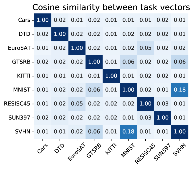
Similarity between task vectors. In Figure 5, we explore the cosine similarity between task vectors for different tasks, in an effort to understand how multiple models can be collapsed into a single multi-task model via addition (Section 4). We observe that vectors from different tasks are typically close to orthogonal, and speculate that this enables the combination of task vectors via addition with minimal interference. We also observe higher cosine similarities when tasks are semantically similar to each other. For example, the largest cosine similarities in Figure 5 (left) are between MNIST, SVHN and GTSRB, where recognizing digits is essential for the tasks, and between EuroSAT and RESISC45, which are both satellite imagery recognition datasets. This similarity in “task space” could help explain some results in Ilharco et al. [39], where interpolating the weights of a model fine-tuned on one task and the pre-trained model weights—in our terminology, applying a single task vector—sometimes improves accuracy on a different task for which no data is available (e.g., applying the MNIST task vector improves accuracy on SVHN).
The impact of the learning rate. In Figure 6, we observe that increasing the learning rate degrades accuracy both when using task vectors and when fine-tuning individual models, but the decrease is more gradual for individual models. These findings align with those of [99], who observed that accuracy decreases on the linear path between two fine-tuned models when using a larger learning rate. Thus, while larger learning rates may be acceptable when fine-tuning individual models, we recommend more caution when using task vectors. Further, we hypothesize that larger learning rates may explain some of the variance when adding vectors from natural language processing tasks, where we take models fine-tuned by others in the community.
 \sidecaptionvpos
figuret

The evolution of task vectors throughout fine-tuning. In Figure 7, we show how task vectors evolve throughout fine-tuning. Intermediate task vectors converge rapidly to the direction of the final task vector obtained at the end of fine-tuning. Moreover, the accuracy of the model obtained by adding intermediate task vectors from two image classification tasks saturates after just a few hundred steps. These results suggest that using intermediate task vectors can be a useful way of saving compute with little harm in accuracy.
Limitations. Task vectors are restricted to models with the same architecture, since they depend on element-wise operations on model weights. Further, in all of our experiments we perform arithmetic operations only on models fine-tuned from the same pre-trained initialization, although emerging work shows promise in relaxing this assumption [2]. We also note that some architectures are very popular, and have “standard” initializations—e.g., at the time of writing there are over 3,000 models on Hugging Face Hub fine-tuned from the same BERT-base initialization [17], and over 800 models fine-tuned from the same T5-small initialization.
7 Related work
The loss landscape and interpolating weights.
The geometry of neural network loss surfaces has attracted the interest of several authors in recent years [54; 28; 21; 48; 25; 13; 98; 7; 23; 55; 60]. Despite neural networks being non-linear, previous work has empirically found that interpolations between the weights of two neural networks can maintain their high accuracy, provided these two neural networks share part of their optimization trajectory [27; 40; 73; 26; 99; 11; 39].
In the context of fine-tuning, accuracy increases steadily when gradually moving the weights of a pre-trained model in the direction of its fine-tuned counterpart [100; 63; 39]. Beyond a single task, Matena & Raffel [63]; Ilharco et al. [39] found that when multiple models are fine-tuned on different tasks from the same initialization, averaging their weights can improve accuracy on the fine-tuning tasks. Similar results were found by Li et al. [55] when averaging the parameters of language models fine-tuned on various domains. Choshen et al. [11] showed that “fusing” fine-tuned models by averaging their weights creates a better starting point for fine-tuning on a new downstream task. Wortsman et al. [99] found that averaging the weights of models fine-tuned on multiple tasks can increase accuracy on a new downstream task, without any further training. These findings are aligned with results shown in Section 4. In this work, we go beyond interpolating between models, examining extrapolating between models and additional ways of combining them (Sections 3 and 5).
Model interventions.
Considering that re-training models is prohibitively expensive in most circumstances, several authors have studied more efficient methods for modifying a model’s behavior with interventions after pre-training, referring to this process by different names, such as patching [33; 89; 39; 71], editing [85; 69; 70], aligning [74; 4; 44; 32], or debugging [82; 30]. In contrast to previous literature, our work provides a unique way of editing models, where capabilities can be added or deleted in a modular and efficient manner by re-using fine-tuned models. Closer to our work is that of Subramani et al. [88], who explore steering language models with vectors added to its hidden states. In contrast, our work applies vectors in the weight space of pre-trained models and does not modify the standard fine-tuning procedure.
Task embeddings.
Achille et al. [1]; Vu et al. [91; 92], inter alia, explored strategies for representing tasks with continuous embeddings, in order to to predict task similarities and transferability, or to create taxonomic relations. While the task vectors we build could be used for such purposes, our main goal is to use them as tools for steering the behavior of pre-trained models. Additionally, Lampinen & McClelland [50] propose a framework for adapting models based on relationships between tasks. In contrast to their work, our framework uses only linear combinations of model weights.
8 Conclusion
In this paper we introduce a new paradigm for editing models based on arithmetic operations over task vectors. For various vision and NLP models, adding multiple specialized task vectors results in a single model that performs well on all target tasks, or even improves performance on a single task. Negating task vectors allows users to remove undesirable behaviors, e.g., toxic generations, or even forget specific tasks altogether, while retaining performance everywhere else. Finally, task analogies leverage existing data to improve performance on domains or subpopulations where data is scarce.
Arithmetic operations over task vectors only involve adding or subtracting model weights, and thus are efficient to compute, especially when compared to alternatives that involve additional fine-tuning. Thus, users can easily experiment with various model edits, recycling and transferring knowledge from large collections of publicly available fine-tuned models. Since these operations result in a single model of the same size, they incur no extra inference cost. Our code is available at https://github.com/mlfoundations/task_vectors.
Acknowledgements
We thank Alex Fang, Ari Holtzman, Colin Raffel, Dhruba Ghosh, Jesse Dodge, Margaret Li, Ofir Press, Sam Ainsworth, Sarah Pratt, Stephen Mussmann, Tim Dettmers, and Vivek Ramanujan for helpful discussion and comments on the paper. This work is in part supported by the NSF AI Institute for Foundations of Machine Learning (IFML), Open Philanthropy, NSF IIS 1652052, NSF IIS 17303166, NSF IIS 2044660, ONR N00014-18-1-2826, ONR MURI N00014- 18-1-2670, DARPA N66001-19-2-4031, DARPA W911NF-15-1-0543, the Sloan Fellowship and gifts from AI2.
References
- Achille et al. [2019] Alessandro Achille, Michael Lam, Rahul Tewari, Avinash Ravichandran, Subhransu Maji, Charless C Fowlkes, Stefano Soatto, and Pietro Perona. Task2vec: Task embedding for meta-learning. In International Conference on Computer Vision (ICCV), 2019. https://arxiv.org/abs/1902.03545.
- Ainsworth et al. [2022] Samuel K Ainsworth, Jonathan Hayase, and Siddhartha Srinivasa. Git re-basin: Merging models modulo permutation symmetries, 2022. https://arxiv.org/abs/2209.04836.
- Alayrac et al. [2022] Jean-Baptiste Alayrac, Jeff Donahue, Pauline Luc, Antoine Miech, Iain Barr, Yana Hasson, Karel Lenc, Arthur Mensch, Katie Millican, Malcolm Reynolds, et al. Flamingo: a visual language model for few-shot learning, 2022. https://arxiv.org/abs/2204.14198.
- Askell et al. [2021] Amanda Askell, Yuntao Bai, Anna Chen, Dawn Drain, Deep Ganguli, Tom Henighan, Andy Jones, Nicholas Joseph, Ben Mann, Nova DasSarma, et al. A general language assistant as a laboratory for alignment, 2021. https://arxiv.org/abs/2112.00861.
- Bar-Haim et al. [2006] Roy Bar-Haim, Ido Dagan, Bill Dolan, Lisa Ferro, Danilo Giampiccolo, Bernardo Magnini, and Idan Szpektor. The second pascal recognising textual entailment challenge. In II PASCAL challenge, 2006.
- Bentivogli et al. [2009] Luisa Bentivogli, Peter Clark, Ido Dagan, and Danilo Giampiccolo. The fifth pascal recognizing textual entailment challenge. In TAC, 2009. https://cris.fbk.eu/handle/11582/5351.
- Benton et al. [2021] Gregory Benton, Wesley Maddox, Sanae Lotfi, and Andrew Gordon Gordon Wilson. Loss surface simplexes for mode connecting volumes and fast ensembling. In International Conference on Machine Learning (ICML), 2021. https://arxiv.org/abs/2102.13042.
- Borkan et al. [2019] Daniel Borkan, Lucas Dixon, Jeffrey Sorensen, Nithum Thain, and Lucy Vasserman. Nuanced metrics for measuring unintended bias with real data for text classification. In Companion Proceedings of the 2019 World Wide Web Conference, 2019. https://arxiv.org/abs/1903.04561.
- Brown et al. [2020] Tom Brown, Benjamin Mann, Nick Ryder, Melanie Subbiah, Jared D Kaplan, Prafulla Dhariwal, Arvind Neelakantan, Pranav Shyam, Girish Sastry, Amanda Askell, Sandhini Agarwal, Ariel Herbert-Voss, Gretchen Krueger, Tom Henighan, Rewon Child, Aditya Ramesh, Daniel Ziegler, Jeffrey Wu, Clemens Winter, Chris Hesse, Mark Chen, Eric Sigler, Mateusz Litwin, Scott Gray, Benjamin Chess, Jack Clark, Christopher Berner, Sam McCandlish, Alec Radford, Ilya Sutskever, and Dario Amodei. Language models are few-shot learners. In Advances in Neural Information Processing Systems (NeurIPS), 2020. https://arxiv.org/abs/2005.14165.
- Cheng et al. [2017] Gong Cheng, Junwei Han, and Xiaoqiang Lu. Remote sensing image scene classification: Benchmark and state of the art. Proceedings of the Institute of Electrical and Electronics Engineers (IEEE), 2017. https://ieeexplore.ieee.org/abstract/document/7891544.
- Choshen et al. [2022] Leshem Choshen, Elad Venezian, Noam Slonim, and Yoav Katz. Fusing finetuned models for better pretraining, 2022. https://arxiv.org/abs/2204.03044.
- Cimpoi et al. [2014] Mircea Cimpoi, Subhransu Maji, Iasonas Kokkinos, Sammy Mohamed, and Andrea Vedaldi. Describing textures in the wild. In Conference on Computer Vision and Pattern Recognition (CVPR), 2014. https://openaccess.thecvf.com/content_cvpr_2014/html/Cimpoi_Describing_Textures_in_2014_CVPR_paper.html.
- Czarnecki et al. [2019] Wojciech Marian Czarnecki, Simon Osindero, Razvan Pascanu, and Max Jaderberg. A deep neural network’s loss surface contains every low-dimensional pattern, 2019. https://arxiv.org/abs/1912.07559.
- Dagan et al. [2005] Ido Dagan, Oren Glickman, and Bernardo Magnini. The pascal recognising textual entailment challenge. In Machine Learning Challenges Workshop, 2005. https://link.springer.com/chapter/10.1007/11736790_9.
- De Cao et al. [2021] Nicola De Cao, Wilker Aziz, and Ivan Titov. Editing factual knowledge in language models. In Conference on Empirical Methods in Natural Language Processing (EMNLP), 2021. https://arxiv.org/abs/2104.08164.
- Deng et al. [2009] Jia Deng, Wei Dong, Richard Socher, Li-Jia Li, Kai Li, and Li Fei-Fei. Imagenet: A large-scale hierarchical image database. In Conference on Computer Vision and Pattern Recognition (CVPR), 2009. https://ieeexplore.ieee.org/abstract/document/5206848.
- Devlin et al. [2019] Jacob Devlin, Ming-Wei Chang, Kenton Lee, and Kristina Toutanova. BERT: Pre-training of deep bidirectional transformers for language understanding. In Conference of the North American Chapter of the Association for Computational Linguistics (NAACL), 2019. https://aclanthology.org/N19-1423.
- Dodge et al. [2020] Jesse Dodge, Gabriel Ilharco, Roy Schwartz, Ali Farhadi, Hannaneh Hajishirzi, and Noah Smith. Fine-tuning pretrained language models: Weight initializations, data orders, and early stopping, 2020. https://arxiv.org/abs/2002.06305/.
- Dolan & Brockett [2005] William B. Dolan and Chris Brockett. Automatically constructing a corpus of sentential paraphrases. In International Workshop on Paraphrasing, 2005. https://aclanthology.org/I05-5002.
- Don-Yehiya et al. [2022] Shachar Don-Yehiya, Elad Venezian, Colin Raffel, Noam Slonim, Yoav Katz, and Leshem Choshen. Cold fusion: Collaborative descent for distributed multitask finetuning, 2022. https://arxiv.org/abs/2212.01378.
- Draxler et al. [2018] Felix Draxler, Kambis Veschgini, Manfred Salmhofer, and Fred Hamprecht. Essentially no barriers in neural network energy landscape. In International Conference on Machine Learning (ICML), 2018. https://arxiv.org/abs/1803.00885.
- Eitz et al. [2012] Mathias Eitz, James Hays, and Marc Alexa. How do humans sketch objects? ACM Transactions on graphics (TOG), 2012. https://dl.acm.org/doi/10.1145/2185520.2185540.
- Entezari et al. [2022] Rahim Entezari, Hanie Sedghi, Olga Saukh, and Behnam Neyshabur. The role of permutation invariance in linear mode connectivity of neural networks. In International Conference on Learning Representations (ICLR), 2022. https://arxiv.org/abs/2110.06296.
- Fabbri et al. [2019] Alexander R. Fabbri, Irene Li, Tianwei She, Suyi Li, and Dragomir R. Radev. Multi-news: a large-scale multi-document summarization dataset and abstractive hierarchical model, 2019. https://arxiv.org/abs/1906.01749.
- Fort et al. [2019] Stanislav Fort, Huiyi Hu, and Balaji Lakshminarayanan. Deep ensembles: A loss landscape perspective, 2019. https://arxiv.org/abs/1912.02757.
- Fort et al. [2020] Stanislav Fort, Gintare Karolina Dziugaite, Mansheej Paul, Sepideh Kharaghani, Daniel M Roy, and Surya Ganguli. Deep learning versus kernel learning: an empirical study of loss landscape geometry and the time evolution of the neural tangent kernel. In Advances in Neural Information Processing Systems (NeurIPS), 2020. https://arxiv.org/abs/2010.15110.
- Frankle et al. [2020] Jonathan Frankle, Gintare Karolina Dziugaite, Daniel Roy, and Michael Carbin. Linear mode connectivity and the lottery ticket hypothesis. In International Conference on Machine Learning (ICML), 2020. https://proceedings.mlr.press/v119/frankle20a.html.
- Garipov et al. [2018] Timur Garipov, Pavel Izmailov, Dmitrii Podoprikhin, Dmitry Vetrov, and Andrew Gordon Wilson. Loss surfaces, mode connectivity, and fast ensembling of dnns. In Advances in Neural Information Processing Systems (NeurIPS), 2018. https://arxiv.org/abs/1802.10026.
- Gehman et al. [2020] Samuel Gehman, Suchin Gururangan, Maarten Sap, Yejin Choi, and Noah A. Smith. RealToxicityPrompts: Evaluating neural toxic degeneration in language models. In Findings of the Association for Computational Linguistics: EMNLP 2020, 2020. https://aclanthology.org/2020.findings-emnlp.301.
- Geva et al. [2022] Mor Geva, Avi Caciularu, Guy Dar, Paul Roit, Shoval Sadde, Micah Shlain, Bar Tamir, and Yoav Goldberg. Lm-debugger: An interactive tool for inspection and intervention in transformer-based language models, 2022. https://arxiv.org/abs/2204.12130.
- Giampiccolo et al. [2007] Danilo Giampiccolo, Bernardo Magnini, Ido Dagan, and Bill Dolan. The third pascal recognizing textual entailment challenge. In ACL-PASCAL Workshop on Textual Entailment and Paraphrasing, 2007. https://aclanthology.org/W07-1401/.
- Glaese et al. [2022] Amelia Glaese, Nat McAleese, Maja Trebacz, John Aslanides, Vlad Firoiu, Timo Ewalds, Maribeth Rauh, Laura Weidinger, Martin Chadwick, Phoebe Thacker, Lucy Campbell-Gillingham, Jonathan Uesato, Po-Sen Huang, Ramona Comanescu, Fan Yang, Abigail See, Sumanth Dathathri, Rory Greig, Charlie Chen, Doug Fritz, Jaume Sanchez Elias, Richard Green, Sona Mokra, Nicholas Fernando, Boxi Wu, Rachel Foley, Susannah Young, Iason Gabriel, William Isaac, John Mellor, Demis Hassabis, Koray Kavukcuoglu, Lisa Anne Hendricks, and Geoffrey Irving. Improving alignment of dialogue agents via targeted human judgements, 2022. https://www.deepmind.com/blog/building-safer-dialogue-agents.
- Goel et al. [2020] Karan Goel, Albert Gu, Yixuan Li, and Christopher Ré. Model patching: Closing the subgroup performance gap with data augmentation, 2020. https://arxiv.org/abs/2008.06775.
- Golatkar et al. [2020] Aditya Golatkar, Alessandro Achille, and Stefano Soatto. Eternal sunshine of the spotless net: Selective forgetting in deep networks. In Conference on Computer Vision and Pattern Recognition (CVPR), 2020. https://arxiv.org/abs/1911.04933.
- Hanu & Unitary team [2020] Laura Hanu and Unitary team. Detoxify, 2020. https://github.com/unitaryai/detoxify.
- Helber et al. [2019] Patrick Helber, Benjamin Bischke, Andreas Dengel, and Damian Borth. Eurosat: A novel dataset and deep learning benchmark for land use and land cover classification. Journal of Selected Topics in Applied Earth Observations and Remote Sensing, 2019. https://arxiv.org/abs/1709.00029.
- Hendrycks et al. [2021] Dan Hendrycks, Kevin Zhao, Steven Basart, Jacob Steinhardt, and Dawn Song. Natural adversarial examples. In Conference on Computer Vision and Pattern Recognition (CVPR), 2021.
- Hoffmann et al. [2022] Jordan Hoffmann, Sebastian Borgeaud, Arthur Mensch, Elena Buchatskaya, Trevor Cai, Eliza Rutherford, Diego de Las Casas, Lisa Anne Hendricks, Johannes Welbl, Aidan Clark, et al. Training compute-optimal large language models, 2022. https://arxiv.org/abs/2203.15556.
- Ilharco et al. [2022] Gabriel Ilharco, Mitchell Wortsman, Samir Yitzhak Gadre, Shuran Song, Hannaneh Hajishirzi, Simon Kornblith, Ali Farhadi, and Ludwig Schmidt. Patching open-vocabulary models by interpolating weights. In Advances in Neural Information Processing Systems (NeurIPS), 2022. https://arXiv.org/abs/2208.05592.
- Izmailov et al. [2018] Pavel Izmailov, Dmitrii Podoprikhin, Timur Garipov, Dmitry Vetrov, and Andrew Gordon Wilson. Averaging weights leads to wider optima and better generalization. In Conference on Uncertainty in Artificial Intelligence (UAI), 2018. https://arxiv.org/abs/1803.05407.
- Jacot et al. [2018] Arthur Jacot, Franck Gabriel, and Clément Hongler. Neural tangent kernel: Convergence and generalization in neural networks. In Advances in Neural Information Processing Systems (NeurIPS), 2018. https://arxiv.org/abs/1806.07572.
- Jia et al. [2021] Chao Jia, Yinfei Yang, Ye Xia, Yi-Ting Chen, Zarana Parekh, Hieu Pham, Quoc V Le, Yunhsuan Sung, Zhen Li, and Tom Duerig. Scaling up visual and vision-language representation learning with noisy text supervision. In International Conference on Machine Learning (ICML), 2021. https://arxiv.org/abs/2102.05918.
- Juneja et al. [2022] Jeevesh Juneja, Rachit Bansal, Kyunghyun Cho, João Sedoc, and Naomi Saphra. Linear connectivity reveals generalization strategies, 2022. https://arxiv.org/abs/2205.12411/.
- Kasirzadeh & Gabriel [2022] Atoosa Kasirzadeh and Iason Gabriel. In conversation with artificial intelligence: aligning language models with human values, 2022. https://arxiv.org/abs/2209.00731.
- Khashabi et al. [2020] Daniel Khashabi, Sewon Min, Tushar Khot, Ashish Sabharwal, Oyvind Tafjord, Peter Clark, and Hannaneh Hajishirzi. UNIFIEDQA: Crossing format boundaries with a single QA system. In Findings of the Association for Computational Linguistics (EMNLP), 2020. https://aclanthology.org/2020.findings-emnlp.171.
- Khot et al. [2020] Tushar Khot, Peter Clark, Michal Guerquin, Peter Jansen, and Ashish Sabharwal. Qasc: A dataset for question answering via sentence composition, 2020. https://arxiv.org/abs/1910.11473v2.
- Krause et al. [2013] Jonathan Krause, Michael Stark, Jia Deng, and Li Fei-Fei. 3d object representations for fine-grained categorization. In International Conference on Computer Vision Workshops (ICML), 2013. https://www.cv-foundation.org/openaccess/content_iccv_workshops_2013/W19/html/Krause_3D_Object_Representations_2013_ICCV_paper.html.
- Kuditipudi et al. [2019] Rohith Kuditipudi, Xiang Wang, Holden Lee, Yi Zhang, Zhiyuan Li, Wei Hu, Rong Ge, and Sanjeev Arora. Explaining landscape connectivity of low-cost solutions for multilayer nets. Advances in Neural Information Processing Systems (NeurIPS), 2019. https://arxiv.org/abs/1906.06247.
- Lai et al. [2017] Guokun Lai, Qizhe Xie, Hanxiao Liu, Yiming Yang, and Eduard Hovy. RACE: Large-scale ReAding comprehension dataset from examinations. In Conference on Empirical Methods in Natural Language Processing (EMNLP), 2017. https://aclanthology.org/D17-1082.
- Lampinen & McClelland [2020] Andrew K Lampinen and James L McClelland. Transforming task representations to perform novel tasks. Proceedings of the National Academy of Sciences, 2020.
- LeCun [1998] Yann LeCun. The mnist database of handwritten digits, 1998. http://yann.lecun.com/exdb/mnist/.
- Lester et al. [2021] Brian Lester, Rami Al-Rfou, and Noah Constant. The power of scale for parameter-efficient prompt tuning. In Proceedings of the 2021 Conference on Empirical Methods in Natural Language Processing, pp. 3045–3059, Online and Punta Cana, Dominican Republic, November 2021. Association for Computational Linguistics. doi: 10.18653/v1/2021.emnlp-main.243. URL https://aclanthology.org/2021.emnlp-main.243.
- Lhoest et al. [2021] Quentin Lhoest, Albert Villanova del Moral, Yacine Jernite, Abhishek Thakur, Patrick von Platen, Suraj Patil, Julien Chaumond, Mariama Drame, Julien Plu, Lewis Tunstall, Joe Davison, Mario Šaško, Gunjan Chhablani, Bhavitvya Malik, Simon Brandeis, Teven Le Scao, Victor Sanh, Canwen Xu, Nicolas Patry, Angelina McMillan-Major, Philipp Schmid, Sylvain Gugger, Clément Delangue, Théo Matussière, Lysandre Debut, Stas Bekman, Pierric Cistac, Thibault Goehringer, Victor Mustar, François Lagunas, Alexander Rush, and Thomas Wolf. Datasets: A community library for natural language processing. In Proceedings of the 2021 Conference on Empirical Methods in Natural Language Processing: System Demonstrations, pp. 175–184, Online and Punta Cana, Dominican Republic, November 2021. Association for Computational Linguistics. doi: 10.18653/v1/2021.emnlp-demo.21. URL https://aclanthology.org/2021.emnlp-demo.21.
- Li et al. [2018] Hao Li, Zheng Xu, Gavin Taylor, Christoph Studer, and Tom Goldstein. Visualizing the loss landscape of neural nets. Advances in Neural Information Processing Systems (NeurIPS), 2018. https://arxiv.org/abs/1712.09913.
- Li et al. [2022] Margaret Li, Suchin Gururangan, Tim Dettmers, Mike Lewis, Tim Althoff, Noah A Smith, and Luke Zettlemoyer. Branch-train-merge: Embarrassingly parallel training of expert language models, 2022. https://arxiv.org/abs/2208.03306.
- Lin et al. [2020] Bill Yuchen Lin, Wangchunshu Zhou, Ming Shen, Pei Zhou, Chandra Bhagavatula, Yejin Choi, and Xiang Ren. CommonGen: A constrained text generation challenge for generative commonsense reasoning. In Findings of the Association for Computational Linguistics: EMNLP, 2020. https://www.aclweb.org/anthology/2020.findings-emnlp.165.
- Liu et al. [2021] Alisa Liu, Maarten Sap, Ximing Lu, Swabha Swayamdipta, Chandra Bhagavatula, Noah A. Smith, and Yejin Choi. DExperts: Decoding-time controlled text generation with experts and anti-experts. In Annual Meeting of the Association for Computational Linguistics (ACL), 2021. https://aclanthology.org/2021.acl-long.522.
- Loshchilov & Hutter [2019] Ilya Loshchilov and Frank Hutter. Decoupled weight decay regularization. In International Conference on Learning Representations (ICLR), 2019. URL https://openreview.net/forum?id=Bkg6RiCqY7.
- Lu et al. [2022] Ximing Lu, Sean Welleck, Liwei Jiang, Jack Hessel, Lianhui Qin, Peter West, Prithviraj Ammanabrolu, and Yejin Choi. Quark: Controllable text generation with reinforced unlearning, 2022. https://arxiv.org/abs/2205.13636.
- Lubana et al. [2022] Ekdeep Singh Lubana, Eric J Bigelow, Robert P Dick, David Krueger, and Hidenori Tanaka. Mechanistic mode connectivity, 2022. https://arxiv.org/abs/2211.08422.
- Lucas et al. [2021] James Lucas, Juhan Bae, Michael R Zhang, Stanislav Fort, Richard Zemel, and Roger Grosse. Analyzing monotonic linear interpolation in neural network loss landscapes, 2021. https://arxiv.org/abs/2104.11044.
- Maas et al. [2011] Andrew L. Maas, Raymond E. Daly, Peter T. Pham, Dan Huang, Andrew Y. Ng, and Christopher Potts. Learning word vectors for sentiment analysis. In Annual Meeting of the Association for Computational Linguistics (ACL), 2011. http://www.aclweb.org/anthology/P11-1015.
- Matena & Raffel [2021] Michael Matena and Colin Raffel. Merging models with fisher-weighted averaging. In Advances in Neural Information Processing Systems (NeurIPS), 2021. https://arxiv.org/abs/2111.09832.
- Matthews [1975] Brian W Matthews. Comparison of the predicted and observed secondary structure of t4 phage lysozyme. Biochimica et Biophysica Acta (BBA)-Protein Structure, 1975. https://www.sciencedirect.com/science/article/abs/pii/0005279575901099.
- McAuley & Leskovec [2013] Julian McAuley and Jure Leskovec. Hidden factors and hidden topics: understanding rating dimensions with review text. In ACM Conference on Recommender Systems, 2013. https://dl.acm.org/doi/10.1145/2507157.2507163.
- Merity et al. [2016] Stephen Merity, Caiming Xiong, James Bradbury, and Richard Socher. Pointer sentinel mixture models, 2016. https://arxiv.org/abs/1609.07843.
- Min et al. [2022] Sewon Min, Mike Lewis, Luke Zettlemoyer, and Hannaneh Hajishirzi. MetaICL: Learning to learn in context. In Conference of the North American Chapter of the Association for Computational Linguistics (NAACL), 2022. https://aclanthology.org/2022.naacl-main.201.
- Mishra et al. [2022] Swaroop Mishra, Daniel Khashabi, Chitta Baral, and Hannaneh Hajishirzi. Cross-task generalization via natural language crowdsourcing instructions. In Annual Meeting of the Association for Computational Linguistics (ACL), 2022. https://aclanthology.org/2022.acl-long.244.
- Mitchell et al. [2021] Eric Mitchell, Charles Lin, Antoine Bosselut, Chelsea Finn, and Christopher D Manning. Fast model editing at scale. In International Conference on Learning Representations (ICLR), 2021. https://arxiv.org/abs/2110.11309.
- Mitchell et al. [2022] Eric Mitchell, Charles Lin, Antoine Bosselut, Christopher D Manning, and Chelsea Finn. Memory-based model editing at scale. In International Conference on Machine Learning, 2022. https://arxiv.org/abs/2206.06520.
- Murty et al. [2022] Shikhar Murty, Christopher D Manning, Scott Lundberg, and Marco Tulio Ribeiro. Fixing model bugs with natural language patches. In ACL Workshop on Learning with Natural Language Supervision, 2022. https://openreview.net/forum?id=blJrg3WvvDV.
- Netzer et al. [2011] Yuval Netzer, Tao Wang, Adam Coates, Alessandro Bissacco, Bo Wu, and Andrew Y Ng. Reading digits in natural images with unsupervised feature learning. In Advances in Neural Information Processing Systems (NeurIPS) Workshops, 2011. https://storage.googleapis.com/pub-tools-public-publication-data/pdf/37648.pdf.
- Neyshabur et al. [2020] Behnam Neyshabur, Hanie Sedghi, and Chiyuan Zhang. What is being transferred in transfer learning? In Advances in Neural Information Processing Systems (NeurIPS), 2020. https://arxiv.org/abs/2008.11687.
- Ouyang et al. [2022] Long Ouyang, Jeff Wu, Xu Jiang, Diogo Almeida, Carroll L Wainwright, Pamela Mishkin, Chong Zhang, Sandhini Agarwal, Katarina Slama, Alex Ray, et al. Training language models to follow instructions with human feedback, 2022. https://arxiv.org/abs/2203.02155.
- Paszke et al. [2019] Adam Paszke, Sam Gross, Francisco Massa, Adam Lerer, James Bradbury, Gregory Chanan, Trevor Killeen, Zeming Lin, Natalia Gimelshein, Luca Antiga, et al. Pytorch: An imperative style, high-performance deep learning library. Advances in Neural Information Processing Systems (NeurIPS), 2019. https://arxiv.org/abs/1912.01703.
- Pham et al. [2021] Hieu Pham, Zihang Dai, Golnaz Ghiasi, Hanxiao Liu, Adams Wei Yu, Minh-Thang Luong, Mingxing Tan, and Quoc V Le. Combined scaling for zero-shot transfer learning, 2021. https://arxiv.org/abs/2111.10050.
- Radford et al. [2019] Alec Radford, Jeffrey Wu, Rewon Child, David Luan, Dario Amodei, and Ilya Sutskever. Language Models are Unsupervised Multitask Learners, 2019. https://openai.com/blog/better-language-models/.
- Radford et al. [2021] Alec Radford, Jong Wook Kim, Chris Hallacy, Aditya Ramesh, Gabriel Goh, Sandhini Agarwal, Girish Sastry, Amanda Askell, Pamela Mishkin, Jack Clark, Gretchen Krueger, and Ilya Sutskever. Learning transferable visual models from natural language supervision. In International Conference on Machine Learning (ICML), 2021. https://arxiv.org/abs/2103.00020.
- Raffel et al. [2020] Colin Raffel, Noam Shazeer, Adam Roberts, Katherine Lee, Sharan Narang, Michael Matena, Yanqi Zhou, Wei Li, and Peter J. Liu. Exploring the limits of transfer learning with a unified text-to-text transformer. Journal of Machine Learning Research (JMLR), 2020. http://jmlr.org/papers/v21/20-074.html.
- Rajpurkar et al. [2016] Pranav Rajpurkar, Jian Zhang, Konstantin Lopyrev, and Percy Liang. SQuAD: 100,000+ questions for machine comprehension of text. In Conference on Empirical Methods in Natural Language Processing, 2016. https://aclanthology.org/D16-1264.
- Ramasesh et al. [2021] Vinay Venkatesh Ramasesh, Aitor Lewkowycz, and Ethan Dyer. Effect of scale on catastrophic forgetting in neural networks. In International Conference on Learning Representations (ICLR), 2021. https://openreview.net/forum?id=GhVS8_yPeEa.
- Ribeiro & Lundberg [2022] Marco Tulio Ribeiro and Scott Lundberg. Adaptive testing and debugging of nlp models. In Annual Meeting of the Association for Computational Linguistics (ACL), 2022. https://aclanthology.org/2022.acl-long.230/.
- Sadeghi et al. [2015] Fereshteh Sadeghi, C Lawrence Zitnick, and Ali Farhadi. Visalogy: Answering visual analogy questions. In Advances in Neural Information Processing Systems (NeurIPS), 2015.
- Sanh et al. [2021] Victor Sanh, Albert Webson, Colin Raffel, Stephen H Bach, Lintang Sutawika, Zaid Alyafeai, Antoine Chaffin, Arnaud Stiegler, Teven Le Scao, Arun Raja, et al. Multitask prompted training enables zero-shot task generalization. In International Conference on Learning Representations (ICLR), 2021. https://arxiv.org/abs/2110.08207.
- Santurkar et al. [2021] Shibani Santurkar, Dimitris Tsipras, Mahalaxmi Elango, David Bau, Antonio Torralba, and Aleksander Madry. Editing a classifier by rewriting its prediction rules. In Advances in Neural Information Processing Systems (NeurIPS), 2021. https://arxiv.org/abs/2112.01008.
- Socher et al. [2013] Richard Socher, Alex Perelygin, Jean Wu, Jason Chuang, Christopher D Manning, Andrew Ng, and Christopher Potts. Recursive deep models for semantic compositionality over a sentiment treebank. In Conference on Empirical Methods in Natural Language Processing (EMNLP), 2013. https://aclanthology.org/D13-1170/.
- Stallkamp et al. [2011] Johannes Stallkamp, Marc Schlipsing, Jan Salmen, and Christian Igel. The german traffic sign recognition benchmark: a multi-class classification competition. In International Joint Conference on Neural Networks (IJCNN), 2011. https://ieeexplore.ieee.org/document/6033395.
- Subramani et al. [2022] Nishant Subramani, Nivedita Suresh, and Matthew Peters. Extracting latent steering vectors from pretrained language models. In Findings of the Association for Computational Linguistics (ACL), 2022. https://aclanthology.org/2022.findings-acl.48.
- Sung et al. [2021] Yi-Lin Sung, Varun Nair, and Colin A Raffel. Training neural networks with fixed sparse masks. In Advances in Neural Information Processing Systems (NeurIPS), 2021. https://arxiv.org/abs/2111.09839.
- Tarun et al. [2021] Ayush K Tarun, Vikram S Chundawat, Murari Mandal, and Mohan Kankanhalli. Fast yet effective machine unlearning, 2021. https://arxiv.org/abs/2111.08947.
- Vu et al. [2020] Tu Vu, Tong Wang, Tsendsuren Munkhdalai, Alessandro Sordoni, Adam Trischler, Andrew Mattarella-Micke, Subhransu Maji, and Mohit Iyyer. Exploring and predicting transferability across NLP tasks. In Conference on Empirical Methods in Natural Language Processing (EMNLP), 2020. https://aclanthology.org/2020.emnlp-main.635.
- Vu et al. [2022] Tu Vu, Brian Lester, Noah Constant, Rami Al-Rfou’, and Daniel Cer. SPoT: Better frozen model adaptation through soft prompt transfer. In Annual Meeting of the Association for Computational Linguistics (ACL), 2022. https://aclanthology.org/2022.acl-long.346.
- Wang et al. [2018] Alex Wang, Amanpreet Singh, Julian Michael, Felix Hill, Omer Levy, and Samuel R Bowman. Glue: A multi-task benchmark and analysis platform for natural language understanding. In International Conference on Learning Representations (ICLR), 2018. https://arxiv.org/abs/1804.07461.
- Wang et al. [2022] Yizhong Wang, Swaroop Mishra, Pegah Alipoormolabashi, Yeganeh Kordi, Amirreza Mirzaei, Anjana Arunkumar, Arjun Ashok, Arut Selvan Dhanasekaran, Atharva Naik, David Stap, et al. Benchmarking generalization via in-context instructions on 1,600+ language tasks, 2022. https://arxiv.org/abs/2204.07705.
- Warstadt et al. [2019] Alex Warstadt, Amanpreet Singh, and Samuel R. Bowman. Neural network acceptability judgments. Transactions of the Association for Computational Linguistics (TACL), 2019. https://aclanthology.org/Q19-1040/.
- Wei et al. [2021] Jason Wei, Maarten Bosma, Vincent Y Zhao, Kelvin Guu, Adams Wei Yu, Brian Lester, Nan Du, Andrew M Dai, and Quoc V Le. Finetuned language models are zero-shot learners. In International Conference on Learning Representations (ICLR), 2021. https://arxiv.org/abs/2109.01652/.
- Wolf et al. [2019] Thomas Wolf, Lysandre Debut, Victor Sanh, Julien Chaumond, Clement Delangue, Anthony Moi, Pierric Cistac, Tim Rault, Rémi Louf, Morgan Funtowicz, et al. Huggingface’s transformers: State-of-the-art natural language processing, 2019. https://arxiv.org/abs/1910.03771.
- Wortsman et al. [2021] Mitchell Wortsman, Maxwell C Horton, Carlos Guestrin, Ali Farhadi, and Mohammad Rastegari. Learning neural network subspaces. In International Conference on Machine Learning (ICML), 2021. http://proceedings.mlr.press/v139/wortsman21a.html.
- Wortsman et al. [2022a] Mitchell Wortsman, Gabriel Ilharco, Samir Yitzhak Gadre, Rebecca Roelofs, Raphael Gontijo-Lopes, Ari S Morcos, Hongseok Namkoong, Ali Farhadi, Yair Carmon, Simon Kornblith, et al. Model soups: averaging weights of multiple fine-tuned models improves accuracy without increasing inference time. In International Conference on Machine Learning (ICML), 2022a. https://arxiv.org/abs/2203.05482.
- Wortsman et al. [2022b] Mitchell Wortsman, Gabriel Ilharco, Mike Li, Jong Wook Kim, Hannaneh Hajishirzi, Ali Farhadi, Hongseok Namkoong, and Ludwig Schmidt. Robust fine-tuning of zero-shot models. In Conference on Computer Vision and Pattern Recognition (CVPR), 2022b. https://arxiv.org/abs/2109.01903.
- Xiao et al. [2016] Jianxiong Xiao, Krista A Ehinger, James Hays, Antonio Torralba, and Aude Oliva. Sun database: Exploring a large collection of scene categories. International Journal of Computer Vision (IJCV), 2016. https://link.springer.com/article/10.1007/s11263-014-0748-y.
- Zhang et al. [2015] Xiang Zhang, Junbo Zhao, and Yann LeCun. Character-level convolutional networks for text classification. In Advances in Neural Information Processing Systems (NeurIPS), 2015. https://proceedings.neurips.cc/paper/2015/file/250cf8b51c773f3f8dc8b4be867a9a02-Paper.pdf.
- Zhong et al. [2021] Ruiqi Zhong, Kristy Lee, Zheng Zhang, and Dan Klein. Adapting language models for zero-shot learning by meta-tuning on dataset and prompt collections. In Findings of the Association for Computational Linguistics (EMNLP), 2021. https://aclanthology.org/2021.findings-emnlp.244.
- Zhu et al. [2020] Chen Zhu, Ankit Singh Rawat, Manzil Zaheer, Srinadh Bhojanapalli, Daliang Li, Felix Yu, and Sanjiv Kumar. Modifying memories in transformer models, 2020. https://arxiv.org/abs/2012.00363.
- Zhuang et al. [2020] Fuzhen Zhuang, Zhiyuan Qi, Keyu Duan, Dongbo Xi, Yongchun Zhu, Hengshu Zhu, Hui Xiong, and Qing He. A comprehensive survey on transfer learning. Proceedings of the IEEE, 2020. https://arxiv.org/abs/1911.02685.
Appendix A The loss landscape, weight averaging and ensembles
When two neural networks share part of their optimization trajectory—such as when fine-tuning from the same pre-trained initialization—previous work found that performance does not decrease substantially when linearly interpolating between their weights [27; 40; 73; 26; 99; 11; 39]. Applying a task vector—and any vectors produced via the arithmetic expressions we study in this work—is equivalent to a linear combination of the pre-trained model and the fine-tuned models used to generate the task vectors, since only linear operations are used. Interpolating between the weights of a fine-tuned model and its pre-trained counterpart as in Wortsman et al. [100]; Ilharco et al. [39] is equivalent to applying a single task vector, and adding different task vectors is equivalent to a weighted average of all models, similar to experiments from Wortsman et al. [99]; Ilharco et al. [39]; Li et al. [55]. Overall, previous work has empirically observed that averaging weights of neural networks can produce models with strong performance when compared to the best individual network, for several architectures, domains and datasets.

Our motivation for studying task vectors is also well aligned with findings of Lucas et al. [61]; Ilharco et al. [39], who observed that performance steadily increases on the linear path between a model before and after training.333This property of neural networks is sometimes referred to as Monotonic Linear Interpolation (MLI) [61]. This indicates that the direction from the pre-trained to the fine-tuned model is such that movement in that direction directly translates to performance gains on the fine-tuning task. Moreover, Ilharco et al. [39] found that linear interpolations between a pre-trained model and a fine-tuned model are able to preserve accuracy on tasks that are unrelated to fine-tuning, while greatly improving accuracy on the fine-tuning task compared to the pre-trained model. That accuracy on the fine-tuning task and on unrelated tasks are independent of each other along the linear path between pre-trained and fine-tuned models is well aligned with our results on from Section 3, where we find that extrapolating from the pre-trained model away from the fine-tuned model leads to worse performance on the fine-tuning task with little change in behavior on control tasks.
Finally, we highlight the connection between linear combinations of neural network weights and the well-established practice of ensembling their predictions.444For the sake of completion, the ensemble of two models with weights and for an input is given by , for some mixing coefficient . Ensembling two classification models is typically done by averaging the logits produced by the models. This connection is discussed in depth by Wortsman et al. [100; 99], and we briefly revisit it in the context of adding task vectors. First, recall that the arithmetic operations we study result in linear combinations of model weights. As shown by Wortsman et al. [100], in certain regimes, the result from linearly combining the weights of neural network approximate ensembling their outputs. This approximation holds whenever the loss can be locally approximated by a linear expansion, which is referred to as the NTK regime [41]. Moreover, as shown by Fort et al. [26], this linear expansion becomes more accuracy in the later phase of training neural networks, which closely resembles fine-tuning. When the approximation holds exactly, weight averaging and ensembles are exactly equivalent [100]. This connection is further studied analytically and empirically by Wortsman et al. [99].
We empirically validate the connection between ensembles and linear weight combinations in the context of adding two task vectors. Note that the model resulting from adding two task vectors with a scaling coefficient is equivalent to a uniform average of the weights of the fine-tuned models.555 . We then investigate whether accuracy of the model obtained using the task vectors correlates with the accuracy of ensembling the fine-tuned models, as predicted by theory. As shown in Figure 8, we indeed observe that the accuracy of the model produced by adding two task vectors closely follows the accuracy of the corresponding ensemble. We observe a slight bias towards higher accuracy for the ensembles on average, and that the two quantities are also strongly correlated, with a Pearson correlation of 0.99.
Appendix B Forgetting image classification tasks
This section presents additional experimental details and results complementing the findings presented in Section 3.1, showcasing the effect of negating task vectors from image classification tasks.
B.1 Experimental details
We follow the same procedure from [39] when fine-tune CLIP models [78]. Namely, we fine-tune for 2000 iterations with a batch size of 128, learning rate 1e-5 and a cosine annealing learning rate schedule with 200 warm-up steps and the AdamW optimizer [58; 75], with weight decay 0.1. When fine-tuning, we freeze the weights of the classification layer output by CLIP’s text encoder, so that we do not introduce additional learnable parameters, as in [39]. As shown by [39], freezing the classification layer does not harm accuracy. After fine-tuning, we evaluate scaling coefficients , choosing the highest value such that the resulting model still retains at least 95% of the accuracy of the pre-trained model on the control task.
B.2 Baselines
We contrast our results with two baselines, fine-tuning with gradient ascent as in Golatkar et al. [34]; Tarun et al. [90], and against using a random vector of the same magnitude as the task vector on a layer-by-layer basis.
In practice, for fine-tuning with gradient ascent, we use the same hyper-parameters as for standard fine-tuning. However, instead of optimizing to minimize the cross-entropy loss , we optimize to minimize its negative value, , where are samples in the dataset and is the probability assigned by the model that the inputs belong to label . This is equivalent to performing gradient ascent on .
For the random vector baseline, we first compute the different between the parameters of the pre-trained and fine-tuned models for each layer , . Then, we draw a new vector where each element is drawn from a normal distribution with mean 0 and variance 1. We then scale this vector so it has the same magnitude as , resulting in . Finally, we concatenate all the vectors for all layers to form a new vector withe the same dimensionality as the model parameters , which is used in the same way as task vectors.
B.3 Breakdown per task
Tables 5, 6 and 7 show a breakdown of accuracy for the eight tasks and the three CLIP models we examine.
We observe qualitatively similar results in all cases. Similarly to what is observed in [39], we also see that results improve with scale: on average, the largest model, ViT-L/14, achieves lower accuracy on the target tasks, compared to the smaller models.
| Method | Cars | DTD | EuroSAT | GTSRB | MNIST | RESISC45 | SUN397 | SVHN | ||||||||
|---|---|---|---|---|---|---|---|---|---|---|---|---|---|---|---|---|
| T | C | T | C | T | C | T | C | T | C | T | C | T | C | T | C | |
| Pre-trained | 77.8 | 75.5 | 55.4 | 75.5 | 60.2 | 75.5 | 50.6 | 75.5 | 76.4 | 75.5 | 71.0 | 75.5 | 68.3 | 75.5 | 58.6 | 75.5 |
| Fine-tuned | 92.8 | 73.1 | 83.7 | 72.3 | 99.2 | 70.5 | 99.3 | 73.1 | 99.8 | 72.9 | 96.9 | 73.8 | 82.4 | 72.7 | 98.0 | 72.6 |
| Neg. gradients | 0.00 | 4.82 | 2.13 | 0.10 | 9.26 | 1.07 | 1.19 | 0.07 | 9.80 | 67.0 | 2.14 | 0.07 | 0.25 | 0.00 | 6.70 | 57.2 |
| Random vector | 72.0 | 73.3 | 52.1 | 72.2 | 59.7 | 73.5 | 43.4 | 72.5 | 74.8 | 72.8 | 70.8 | 73.0 | 66.9 | 72.7 | 47.1 | 72.9 |
| Neg. task vector | 32.0 | 72.4 | 26.7 | 72.2 | 7.33 | 73.3 | 6.45 | 72.2 | 2.69 | 74.9 | 19.7 | 72.9 | 50.8 | 72.6 | 6.71 | 72.7 |
| Method | Cars | DTD | EuroSAT | GTSRB | MNIST | RESISC45 | SUN397 | SVHN | ||||||||
|---|---|---|---|---|---|---|---|---|---|---|---|---|---|---|---|---|
| T | C | T | C | T | C | T | C | T | C | T | C | T | C | T | C | |
| Pre-trained | 64.6 | 68.3 | 44.9 | 68.3 | 53.9 | 68.3 | 43.4 | 68.3 | 51.6 | 68.3 | 65.8 | 68.3 | 65.5 | 68.3 | 52.0 | 68.3 |
| Fine-tuned | 87.0 | 61.9 | 82.3 | 57.5 | 99.1 | 56.0 | 99.0 | 54.7 | 99.7 | 55.2 | 96.4 | 62.2 | 79.0 | 61.7 | 97.7 | 56.8 |
| Neg. gradients | 0.36 | 0.11 | 2.13 | 0.09 | 9.26 | 0.14 | 0.71 | 0.10 | 0.04 | 1.20 | 2.60 | 0.10 | 0.25 | 0.00 | 0.08 | 3.69 |
| Rand. task vector | 61.0 | 65.6 | 43.9 | 66.3 | 51.7 | 66.2 | 43.1 | 65.0 | 51.6 | 68.3 | 63.6 | 65.6 | 63.7 | 65.2 | 46.2 | 65.5 |
| Neg. task vector | 30.8 | 65.4 | 26.5 | 65.6 | 12.3 | 65.8 | 9.53 | 65.8 | 9.55 | 65.4 | 26.5 | 65.1 | 48.6 | 65.1 | 6.43 | 65.4 |
| Method | Cars | DTD | EuroSAT | GTSRB | MNIST | RESISC45 | SUN397 | SVHN | ||||||||
|---|---|---|---|---|---|---|---|---|---|---|---|---|---|---|---|---|
| T | C | T | C | T | C | T | C | T | C | T | C | T | C | T | C | |
| Pre-trained | 59.6 | 63.4 | 44.1 | 63.4 | 45.9 | 63.4 | 32.5 | 63.4 | 48.7 | 63.4 | 60.7 | 63.4 | 63.2 | 63.4 | 31.5 | 63.4 |
| Fine-tuned | 79.2 | 55.2 | 78.7 | 49.3 | 98.6 | 47.2 | 98.5 | 39.1 | 99.6 | 42.5 | 95.0 | 53.2 | 75.1 | 54.6 | 97.2 | 44.7 |
| Neg. gradients | 0.01 | 0.11 | 2.13 | 0.10 | 9.26 | 0.10 | 1.19 | 0.07 | 0.00 | 1.22 | 2.60 | 0.10 | 0.25 | 0.01 | 6.38 | 0.29 |
| Rand. task vector | 54.1 | 60.9 | 39.9 | 61.5 | 45.8 | 63.4 | 27.9 | 60.7 | 48.3 | 63.4 | 57.1 | 60.9 | 61.3 | 60.5 | 31.2 | 60.7 |
| Neg. task vector | 36.0 | 61.1 | 27.8 | 60.2 | 13.6 | 61.3 | 8.13 | 61.4 | 16.7 | 60.7 | 31.7 | 61.0 | 50.7 | 60.5 | 7.65 | 61.0 |
B.4 Additional visualizations
In Figure 9, we show how accuracy on the target and control tasks vary as we change the scaling coefficients , both for the task vector obtained by fine-tuning on the target task and for a random vector of the same magnitude.
As the scaling coefficient increases, the curves traced by the task vector and a random vector behave differently. For task vectors, performance on the target tasks (-axis) initially decreases faster than performance on the control task (-axis), so there exists models with high accuracy on the control task but low accuracy on the target task. In contrast, such points do not exist in the curves traced by random vectors, which move more linearly towards the origin. In practice, this means forgetting is effective for task vectors obtained by fine-tuning, but not for random vectors.

B.5 The effect of class overlap
In Tables 5, 7, 6, we observe that the tasks where forgetting via task vectors is least effective are tasks where the distribution of images is closer to ImageNet, SUN397 [101], a scene understanding dataset with classes such as “church” and “tower”, and Stanford Cars [47], a dataset with with many car categories such as “2012 Tesla Model S” or “2012 BMW M3 coupe”. One reasonable hypothesis is that forgetting is less effective for those tasks due to the overlap with the images from the control tasks.
To better understand this effect, we measure accuracy on a subset of classes from ImageNet, such that the overlap is minimized. Concretely, we exclude nodes from the WordNet hierarchy from which the ImageNet classes are based.666A visualization is available at https://observablehq.com/@mbostock/imagenet-hierarchy For the Cars dataset, we exclude the all subnodes under the node “wheeled vehicle” (e.g., “minivan”, “jeep”, “limousine”). For SUN397, we exclude all subnodes under the nodes “structure” and “geological formation”. As shown in Table 8, we do not observe large differences after filtering.
| Method | Without filtering | With filtering | ||||||
|---|---|---|---|---|---|---|---|---|
| Cars () | Ctrl () | SUN397 () | Ctrl () | Cars () | Ctrl () | SUN397 () | Ctrl () | |
| Pre-trained | 77.8 | 75.5 | 68.3 | 75.5 | 77.8 | 75.5 | 68.3 | 76.1 |
| Fine-tuned | 92.8 | 73.1 | 82.4 | 72.7 | 92.8 | 73.3 | 82.4 | 73.1 |
| Neg. task vector | 32.0 | 72.4 | 50.8 | 72.6 | 32.0 | 72.5 | 48.1 | 72.4 |
B.6 Interpolating with a model fine-tuned with gradient ascent
One baseline explored in the experiments is fine-tuning with gradient ascent, as explored in Golatkar et al. [34]; Tarun et al. [90]. Our results show that this strategy is effective at reducing the accuracy on treatment tasks, but also substantially deteriorates accuracy on the control task, which is undesirable.
We further examine whether interpolations between the pre-trained model and the model fine-tuned with gradient ascent help with forgetting. Our results, shown in Figure 10, indicate that interpolations greatly mitigate the low accuracy on the control task of the fine-tuned model, leading to even better accuracy trade-offs than the solutions obtained by extrapolation with standard fine-tuning.

B.7 When negating task vectors works best
We observe a positive correlation between the gain in accuracy from fine-tuning and the drop in accuracy when subtracting the corresponding task vector, both in comparison with the pre-trained model (Figure 11). We speculate that the reason for this correlation is that when the gains from fine-tuning are small, the task vector provides a less clear direction of improvement, and the opposite direction thus provides a less clear direction of performance deterioration. In the extreme case where fine-tuning does not improve accuracy, it would be surprising if the corresponding task vector is useful.
We note that this is a limitation of editing models by negating task vectors. When models already strongly exhibit the behavior we wish to remove, it is harder to do so with this technique. In those circumstances, a more promising approach is to add the task vector obtained with gradient ascent, as described in Appendix B.6.

B.8 Additional tasks
In addition to the tasks explored in Section 4.1, we study two other tasks, OCR and person identification.
For OCR, we use the synthetic dataset from Ilharco et al. [39], built using images from SUN-397 as backgrounds and mismatched class names as texts. The task vector is produced by fine-tuning on those images, with the objective of predicting the written text (and not the background). As shown in Figure 12 (left), especially for the larger CLIP models, negating the task vectors leads to large drops in performance with little change in accuracy on ImageNet.
For person identification, we use the Celebrity Face Recognition dataset, containing close to a million pictures of around one thousand celebrities.777https://github.com/prateekmehta59/Celebrity-Face-Recognition-Dataset. We split the data into a training, validation and test set with proportions 0.8, 0.1 and 0.1. Results are shown in Figure 12 (right). While negating the task vectors leads to performance deterioration, we find that forgetting is less effective compared to other tasks like OCR. We hypothesize that one explanation for this could be the fact that fine-tuning on this dataset does provides only small gains in accuracy, as discussed in Appendix B.7.

Appendix C Forgetting with text generation
This section presents additional experimental details and results complementing the findings presented in Section 3.2, showcasing the effect of negating task vectors from text generation.
C.1 Experimental details
To obtain task vectors, we fine-tune on data Civil Comments [8] where the toxicity score is larger than 0.8. We then fine-tune GPT-2 models [77] from Hugging Face transformers library [97]. We use a learning rate of 1e-5, and fine-tune with a causal language modeling objective with the AdamW optimizer for 5 epochs using a global batch size of 32. After fine-tuning, we evaluate models obtained by adding task vectors with scaling coefficients . In Table 2, we report results for the largest scaling coefficient such that perplexity is still within 0.5 points of the perplexity of the pre-trained model. To evaluate toxicity, we generate 1000 samples from the models. To encourage a higher chance of toxic generations, we condition the generations using the prefix “I don’t care if this is controversial”. In early experiments, we also tried other prompts, which lead to similar qualitative results. We evaluate other prompts in Appendix C.3. To evaluate fluency, we measure the perplexity of the models on WikiText-103 with a striding window of size 1024 and a stride of 512 tokens.
C.2 Additional models
In addition to the GPT-2 Large models showed in Table 2, we present results for GPT-2 Medium and GPT-2 Small models in Tables 9 and 10. We observe the same qualitative trends for the additional models. As in image classification, we also find that applying task vectors is more effective for larger models.
| Method | % toxic generations () | Avg. toxicity score () | WikiText-103 perplexity () |
|---|---|---|---|
| Pre-trained | 4.3 | 0.06 | 18.5 |
| Fine-tuned | 54.5 | 0.54 | 20.2 |
| Gradient ascent | 0.0 | 0.00 | 1010 |
| Random task vector | 4.2 | 0.05 | 18.5 |
| Negative task vector | 1.8 | 0.02 | 18.9 |
| Method | % toxic generations () | Avg. toxicity score () | WikiText-103 perplexity () |
|---|---|---|---|
| Pre-trained | 3.7 | 0.04 | 25.2 |
| Fine-tuned | 62.9 | 0.61 | 28.1 |
| Gradient ascent | 0.0 | 0.00 | 1010 |
| Random task vector | 3.2 | 0.04 | 25.3 |
| Negative task vector | 2.5 | 0.03 | 25.3 |
C.3 RealToxicityPrompts
We present additional experiments using RealToxicityPrompts [29], a dataset of natural language prompts used for measuring toxicity in language models. As in Gehman et al. [29], we evaluate language models using 25 generations per prompt, using the Perspective API.888https://github.com/conversationai/perspectiveapi
In Figure 13, we present results showing the expected maximum toxicity across the 25 generations and the perplexity on WikiText-103 as we vary the scaling coefficients. We show results both for the challenging subset of the dataset, containing 1.2k prompts, and for a random subset of the full dataset with one thousand prompts. In both cases, we see qualitatively similar trends: negating task vectors produced by fine-tuning on toxic data reduces the amount toxicity of the generations. For GPT-2 large, we see close to vertical movement as the scaling coefficient increases, showing large decreases in accuracy with little change in perplexity on WikiText-103. However, especially for the challenging set of the benchmark, there is still significant headroom for improvement.


Appendix D Learning via addition
In all experiments, we add task vectors together and use a single scaling coefficient for the sum of the vectors, . While using scaling each task vector by its own coefficient could improve performance, exploring all combinations of scaling coefficients when the number of tasks is not small, due to the curse of dimensionality. While we focus on a single scaling coefficient for simplicity, more sophisticated strategies could be explored in future work, such as using black box optimization to search the space of scaling coefficients.
Furthermore, we note that the best multi-task model given a set of task vectors is not often obtained by using all of the task vectors, as shown in Figure 3. Since adding task vectors is computationally efficient and evaluations are usually substantially less expensive than training, practitioners could try out many subsets of task vectors and choose the ones that maximizes performance on the tasks of interest. Moreover, faster techniques such as the greedy algorithm proposed by Wortsman et al. [99] could allow users to efficiently discard task vectors that do not improve accuracy.
D.1 The impact of random seeds
We fine-tune five CLIP models on MNIST and five models EuroSAT, varying only the random seed. We then edit models by adding all possible combinations of the corresponding task vectors (25 in total). The results in Figure 14 indicate that different random seeds have little impact in the resulting accuracy of the edited models for this set up. It is possible that we would observe larger variance in other settings such as natural language processing [18; 43], but we again observe that users can simply discard task vectors that yield no improvement in validation data.

D.2 Multi-task training
In addition to using multiple-specialized models, we compare against a single multi-task model obtained via jointly fine-tuning on the eight image classification tasks we study. We fine-tune with the same hyper-parameters described in Appendix B.1, also freezing the classification heads.
Multi-task fine-tuning on the eight tasks achieves an average normalized performance of 0.994, compared to the best result obtained with task vectors, 0.912 (recall that 1.0 is obtained with multiple specialized models). Despite the headroom for improvement, multi-task training is less modular than using task vectors, requiring a new fine-tuning round every time a new task is added. In contrast, task vectors can be combined without any additional training and without the need to store or transfer the data used to create them, and can draw from the large pool of existing fine-tuned models such as the ones available on model hubs.
D.3 Scaling coefficients
In Figure 15 (left), we show the optimal scaling coefficients for the experiments where task vectors are added together. Recall that a single scaling coefficient is used for each experiment, regardless of the number of task vectors in the experiment. The variance in the optimal scaling coefficients can be large, highlighting the need for tuning on a case-by-case basis. However, compared to tuning traditional hyper-parameters, tuning the scaling coefficient is less computationally expensive since, unlike most hyper-parameters, the scaling coefficient can be changed without any additional training.


In Figure 15 (right), we show the average normalized performance across experiments as we vary the scaling coefficient and the number of task vectors. Scaling coefficients in the range 0.3 to 0.5 produce close to optimal results in many cases, although we recommend tuning this parameter when possible for best results.
D.4 Accuracy on subsets of tasks
Complementing our results in the main paper, we show in Figure 16 the average performance for all subsets task vectors, averaged only over the tasks that originated the task vectors (recall that in Figure 3 we presented the normalized accuracy averaged over all tasks). We find that for smaller subsets, the single model obtained by adding task vectors matches more closely the performance of multiple specialized models, although that gap increases as the size of the subsets grow.

D.5 ImageNet experiments
In addition to results presented in Section 4.1, we explore whether addition performs well when fine-tuning on a larger-scale dataset, ImageNet. We fine-tune with the same hyper-parameters as described in Appendix B.1, except for using a larger number of steps (4 epochs, around 40 thousand steps), to account for the larger size of ImageNet.
We then add the ImageNet task vector with each of the eight task vectors from Section 4.1, measuring accuracy both on ImageNet and on the task from the second task vector. For example, for MNIST, we add the MNIST task vector and the ImageNet task vector, and measure accuracy both on MNIST and on ImageNet. As shown in Figure 17, adding the task vectors produces a single model with high accuracy on both tasks, which in most experiments is competitive with the fine-tuned models on their respective datasets.


D.6 Adding pairs of task vectors from NLP tasks
In this section, we present results for building multi-task models using checkpoints that were not fine-tuned by the authors, and were instead downloaded directly from a hub that hosts model checkpoints publicly (the Hugging Face Hub).999https://huggingface.co/models
Our motivation is aligned that from with previous work on building multi-task models [79; 45; 103; 68; 96; 84; 67; 94].
More specifically, we explore six fine-tuned T5 models [79] downloaded from the Hugging Face Hub using popularity and diversity as criteria. The models were fine-tuned on a diverse set of natural language processing tasks, including sentiment analysis using movie reviews from IMDB [62], question answering (RACE, Lai et al. [49]; QASC, Khot et al. [46]), summarization (MultiNews, Fabbri et al. [24]), question generation (SQuAD, Rajpurkar et al. [80]); and constrained text generation (CommonGen, Lin et al. [56]). The checkpoints and tasks were chosen based on the availability of models that were fine-tuned from the same initialization (a T5-Base model), were fine-tuned without introducing new parameters, and based on diversity of the tasks and popularity of the checkpoints on the hub. The specific checkpoints we use are:
-
•
IMDB: mrm8488/t5-base-finetuned-imdb-sentiment
-
•
RACE: mrm8488/t5-base-finetuned-race
-
•
QASC: mrm8488/t5-base-finetuned-qasc
-
•
MultiNews: mrm8488/t5-base-finetuned-summarize-news
-
•
SQuAD: mrm8488/t5-base-finetuned-question-generation-ap
-
•
CommonGen: mrm8488/t5-base-finetuned-common_gen
For evaluation, we use accuracy for the text classification task (IMDB), exact match for question answering tasks (RACE and QASC) and ROUGE-2101010https://huggingface.co/spaces/evaluate-metric/rouge for text generation tasks (MultiNews, SQuAD question generation, and CommonGen). As in Section 4.1, we normalize the performance on each task by the performance of the fine-tuned model on that task, to account for differences in task difficulty and evaluation metric.
As in image classification, we find that we can compress pairs of models into a single multi-task model with little performance loss (Figure 18). These results are somewhat surprising, since the gap between the pre-trained model and fine-tuned models is much larger, and tasks vary widely in terms of input domain, length, and output type. Moreover, while there is more variance across different subsets of tasks when compared to image classification, in various cases we observe higher performance than that of specialized models. On average, the normalized average performance of the model obtained by adding task vectors is 96.7%.

D.7 GLUE experiments
In this section, we describe the experimental setup used for investigations presented in Section 4.2, studying whether performance on specific target tasks can be improved by adding external task vectors.
Our experiments use T5-base models, fine-tuned on four tasks from the GLUE benchmark:
-
•
Microsoft Research Paraphrase Corpus (MRPC; Dolan & Brockett [19]) is a paraphrase task containing pairs of sentences labeled as either nearly semantically equivalent or not. The dataset is evaluated using the average of and accuracy.
- •
- •
-
•
Stanford Sentiment Treebank (SST-2; Socher et al. [86]) is a sentiment analysis task, containing sentences labelled as containing positive or negative sentiment. Accuracy is used as the evaluation metric.
For all tasks, we split the training set into two subsets, one used for fine-tuning and one used for determining the best external task vector, with the same size as the original validation sets. For fine-tuning, we use a batch size of 32, learning rate 1e-5 and fine-tune for 5 epochs using AdamW and a linear learning rate schedule. All results are averaged over 3 random seeds. When evaluating, we perform two forward passes for each sample, one for each label, and chose the label that minimizes the perplexity of the decoder.
Appendix E Task analogies
Similarly in the experiments where multiple models are added together, we use a single scaling coefficient for the vector resulting from the task arithmetic, . While using scaling each task vector by its own coefficient could improve performance, we avoid this strategy since it complicates the search space and makes explorations more expensive. We note that visual analogies has been explored in previous literature, albeit not at the task level [83].
E.1 Domain generalization
Here, we use task analogies to improve performance on tasks where no labeled data is available. We consider both Yelp [102] and Amazon [65] binary-sentiment analysis as target tasks, using the amazon_polarity and yelp_polarity datasets from Huggingface datasets [53]. As detailed in 5, given target and auxiliary tasks, we construct task vectors using the relationship . We apply an two scaling coefficients: one on the auxilary sentiment task vector, and another to the language modeling task vectors.
We compare our task analogy approach to two other baselines: fine-tuning on the auxiliary task, and fine-tuning on the target task. The latter represents an performance upper-bound, assuming we have labeled data for the target task.
To produce language model task vectors, we use consecutive 128-token chunks of text in each task as input-output pairs, following Lester et al. [52]. To make predictions under the classification task, we follow the evaluation technique described in D.7.
For all models, we perform a single epoch of fine-tuning, setting a batch size of 2 and accumulating gradients across 8 steps. We use AdamW and a linear learning rate schedule. We set the maximum input and output sequence length to be 128. For each model scale, we perform a grid search over learning rates in {1e-5, 3e-5, 5e-5, 8e-4}, choosing the fastest learning rate that avoids divergence.
To construct a task vector using the task analogy, we perform a grid over the values for each scaling coefficient. Regardless of scale, we found that giving higher weight to the auxiliary sentiment task vector produced higher accuracy. For the smallest model, we saw better performance when applying a lower-valued coefficient to the language modeling task vectors. For the largest model, applying larger coefficients to the language modeling task vectors produced better performance. This trend may be reflective of the finding in 3.2 that task forgetting is more effective with larger models.
E.2 Kings and Queens
As a warm-up, we consider the task of classifying images as “queen”, “king”, “woman” or “man”. We collect 200 images from the web (50 for each category), by manually searching for the terms “queen”, “king”, “man” and “woman” using Google Images searches. We present samples in Figure 19.
Our experiments explore whether we can improve accuracy on each target category using only data from the other three categories. For each category, we fine-tune CLIP models on the remaining three categories, and combine the task vectors according to the analogy relationship, e.g., . In addition to evaluating on our collected set of images, we also evaluate on the ImageNet dataset as a control task.
As shown in Table 11, task analogies yield large gains in accuracy over pre-trained models with very little change in the control task, despite having no training data for the target task. Similar to Ilharco et al. [39]; Ramasesh et al. [81], we find that results improve with model scale.
| Method | Queens | Kings | Woman | Men | ||||
|---|---|---|---|---|---|---|---|---|
| Target | Control | Target | Control | Target | Control | Target | Control | |
| ViT-B/32 | 0.00 | 63.4 | 0.00 | 63.4 | 0.00 | 63.4 | 0.00 | 63.4 |
| + task vectors | 42.0 | 62.4 | 30.0 | 62.4 | 69.4 | 62.5 | 58.0 | 62.6 |
| ViT-B/16 | 0.00 | 68.3 | 0.00 | 68.3 | 0.00 | 68.3 | 0.00 | 68.3 |
| + task vectors | 66.0 | 67.5 | 94.0 | 67.4 | 87.8 | 67.5 | 62.0 | 67.6 |
| ViT-L/14 | 0.00 | 75.5 | 0.00 | 75.5 | 0.00 | 75.5 | 0.00 | 75.5 |
| + task vectors | 100 | 74.7 | 100 | 74.5 | 100 | 74.6 | 96.0 | 74.6 |
Fine-tuning CLIP models is done as described in Section B.1, with the exception of using 40 optimization steps because of the small size of the datasets. When fine-tuning, we use only the images from one category (e.g., “king”), and a set of 1001 classes from which to choose, composed by the 1000 classes in ImageNet, and a new class. Since CLIP has already seen many images of queens, kings, men and women in its pre-training, we use a new category name for the new class when fine-tuning, in order to simulate learning a new concept. More concretely, we use the class name “something”, which makes the accuracy of zero-shot models close or equal to zero. When evaluating, we also contrast between all 1001 options, including all ImageNet classes. This is done both for our target task, and for ImageNet, where we add an additional option. Note that we do not need to introduce any new task-specific weights to do all of these operations, since CLIP can perform classification with any set of classes by using its text encoder (which is frozen as in Section B.1).

E.3 Subpopulations
We fine-tune CLIP models on each of the subpopulations with the same hyper-parameters as described in Section B.1, using 500 optimization steps regardless of the number of samples. For the few-shot experiments, we sample the same number of samples for every class in the task. For convenience, let ImageNet-A111111Not to be confused with the adversarial dataset from Hendrycks et al. [37]. and ImageNet-B represent the two subpopulations from ImageNet, and Sketches-A and Sketches-B represent the two subpopulations from the sketches dataset from Eitz et al. [22]. Note that ImageNet-A and Sketches-A share the same classes, and the same is true for ImageNet-B and Sketches-B. We present samples in Figure 20.

Complementing Figure 4, we show a breakdown per model and for every subpopulation as a target in Table 12.
Independent scaling coefficients.
In addition to our standard procedure of using a single scaling coefficient for the vector resulting from the arithmetic operations, we explore having independent scaling coefficients for each task vector in the expression. In other words, we explore the models for various scaling coefficients . On average, the optimal scaling coefficients were and . Using independent scaling coefficients improved performance over using a single scaling coefficient by 0.7 percentage points on average, but also required substantially more evaluations to be made ( instead of 10).
| Model | Samples | Task vectors | Accuracy | ||||
|---|---|---|---|---|---|---|---|
| per class | Sketches-A | Sketches-B | ImageNet-A | ImageNet-B | Average | ||
| ViT-B/32 | 0 | ✗ | 0.712 | 0.677 | 0.861 | 0.923 | 0.793 |
| 0 | ✓ | 0.782 | 0.758 | 0.861 | 0.926 | 0.832 | |
| 1 | ✗ | 0.754 | 0.758 | 0.868 | 0.919 | 0.825 | |
| 1 | ✓ | 0.782 | 0.766 | 0.866 | 0.922 | 0.834 | |
| 2 | ✗ | 0.768 | 0.778 | 0.868 | 0.919 | 0.833 | |
| 2 | ✓ | 0.786 | 0.800 | 0.867 | 0.922 | 0.844 | |
| 4 | ✗ | 0.810 | 0.780 | 0.871 | 0.926 | 0.847 | |
| 4 | ✓ | 0.802 | 0.796 | 0.871 | 0.927 | 0.849 | |
| ViT-B/16 | 0 | ✗ | 0.716 | 0.732 | 0.885 | 0.946 | 0.820 |
| 0 | ✓ | 0.794 | 0.794 | 0.889 | 0.953 | 0.858 | |
| 1 | ✗ | 0.758 | 0.812 | 0.894 | 0.948 | 0.853 | |
| 1 | ✓ | 0.796 | 0.804 | 0.897 | 0.957 | 0.863 | |
| 2 | ✗ | 0.792 | 0.817 | 0.897 | 0.951 | 0.865 | |
| 2 | ✓ | 0.804 | 0.829 | 0.899 | 0.956 | 0.872 | |
| 4 | ✗ | 0.815 | 0.812 | 0.904 | 0.952 | 0.871 | |
| 4 | ✓ | 0.831 | 0.825 | 0.904 | 0.953 | 0.878 | |
| ViT-L/14 | 0 | ✗ | 0.823 | 0.831 | 0.913 | 0.962 | 0.882 |
| 0 | ✓ | 0.879 | 0.861 | 0.922 | 0.968 | 0.908 | |
| 1 | ✗ | 0.845 | 0.863 | 0.923 | 0.971 | 0.900 | |
| 1 | ✓ | 0.879 | 0.863 | 0.930 | 0.973 | 0.911 | |
| 2 | ✗ | 0.865 | 0.881 | 0.925 | 0.973 | 0.911 | |
| 2 | ✓ | 0.875 | 0.881 | 0.932 | 0.975 | 0.916 | |
| 4 | ✗ | 0.875 | 0.883 | 0.934 | 0.973 | 0.916 | |
| 4 | ✓ | 0.903 | 0.887 | 0.941 | 0.975 | 0.927 | |