Edge adaptive hybrid regularization model for image deblurring
Abstract
The parameter selection is crucial to regularization based image restoration methods. Generally speaking, a spatially fixed parameter for regularization item in the whole image does not perform well for both edge and smooth areas. A larger parameter of regularization item reduces noise better in smooth areas but blurs edge regions, while a small parameter sharpens edge but causes residual noise. In this paper, an automated spatially adaptive regularization model, which combines the harmonic and TV models, is proposed for reconstruction of noisy and blurred images. In the proposed model, it detects the edges and then spatially adjusts the parameters of Tikhonov and TV regularization terms for each pixel according to the edge information. Accordingly, the edge information matrix will be also dynamically updated during the iterations. Computationally, the newly-established model is convex, which can be solved by the semi-proximal alternating direction method of multipliers (sPADMM) with a linear-rate convergence rate. Numerical simulation results demonstrate that the proposed model effectively reserves the image edges and eliminates the noise and blur at the same time. In comparison to state-of-the-art algorithms, it outperforms other methods in terms of PSNR, SSIM and visual quality.
, , , , and
Keywords: the edge information matrix, image deblurring, semi-proximal alternating direction method of multipliers
1 Introduction
Images are frequently degraded by noise and blurring during the image acquisition and transmission procedures [23, 36]. As a result, image denoising and deblurring are two fundamental steps for various image processing tasks, such as image segmentation, edge detection, and pattern recognition. Let be the unknown clear image of size , and be the observed degraded image with Gaussian white noise. Then the mathematical model for image degradation [1, 3, 21, 25] is formulated as follows,
| (1.1) |
where is the known blurring operator, is the convolution of with as
Moreover, represents the Gaussian white noise with mean and standard deviation . Let denotes the vector space of 2D images defined on . For each 2D image , the total number of pixels is , and denotes the image value at pixel . Restoring the unknown image from the degraded image is a typical ill-posed problem. Hence, effective image deblurring methods usually rely on delicately designed regularizations based on the prior information on .
To preserve significant edges, Rudin, Osher, and Fatemi[38] proposed the celebrated total variation (TV) model for image restoration. By this approach, the recovery of the image is based on solving the following minimization problem
| (1.2) |
where is the gradient in the discrete setting with , and and denote the horizontal and vertical first-order differences with Dirichlet boundary condition respectively, which are defined as follows
| (1.3) |
and is the -norm of
| (1.4) |
As the total variation term is powerful for preserving sharp edges, the TV model has been widely used for image processing. Over the past years, much effort has been devoted to studying, solving and extending the TV model. In particular, a two-phase approach for deblurring images [6, 7] was proposed to handle the impulsive noise. More related models and algorithms have been reported in [9, 10, 11, 12, 16, 20, 24, 33, 35, 37, 34, 40, 43, 44, 45, 46].
However, image deblurring with TV model often leads to some undesirable staircase effects, namely, the transformation of smooth regions into piece-wise constant ones. There are at least two possible ways to handle this issue. One is to use the tight-frame approaches [9, 10]. The other is to combine the TV regularization term with some more advanced models. For instance, the harmonic model [39] with Tikhonov regularization and fourth-order PDE (LLT) filter [32] can effectively reduce noise. Therefore, some hybrid regularization models combining the TV model with LLT models [26, 29, 32, 37] or harmonic models [19, 30] are proposed to preserve edges while restraining the staircase effects at the same time. Furthermore, Liu et al.[28] combines image sharpening operator and framelet regularization [8] for image deblurring, whose model is expressed as,
| (1.5) |
where is the framelet transformation, is a sharpened image, and are positive parameters. In the optimization problem (1.2), the positive parameter controls the trade-off between a good fit of and a smoothness requirement by the total variation regularization. In general, an image is composed of multiple objects at different scales. This suggests that different values of are desirable for various image features of different scales, to obtain better results. More specifically, for the texture regions, we can use larger as it leads to less smoothed and more detailed restoration. On the other hand, for the flat region, smaller is desired to get a better smoothing and noise-reduced result. For this reason, in [2, 4] the multi-scale total variation (MTV) models were proposed, with spatially varying parameters based on (1.2). The corresponding multi-scale version of model (1.2) is represented as
| (1.6) |
where is spatially varying non-negative parameter matrix, . As in Matlab, denotes point-wise product between the elements and as follows,
| (1.7) |
Borrowing the idea of (1.6), the multi-scale technique can be applied to the TV term, which yields
| (1.8) |
where is a non-negative spatially varying parameter matrix, is given by
| (1.9) |
Introducing a local parameter gives more flexibility to the model in exchange for the robustness. For this reason, Dong et al.[17] proposed a method to decide whether to use a spatially varying parameter, by using a confidence interval technique based on the expected maximal local variance estimate. In this paper, we study the properties of the image edges and propose an edge adaptive hybrid regularization model by introducing an edge detection operation to a combination of the TV and harmonic models. The edge detection operation is used to decide, in a robust way, where the edges are located in the noisy image and generates an edge information matrix. This edge information matrix, is later applied to decide the acceptance or rejection of a scaling parameter. It is worth to mention that our edge information matrix is obtained and updated fully automatically in each iteration for preserving edges. Furthermore, the proposed model is convex once the local parameters are fixed, and hence it can be solved efficiently by the semi-proximal alternating direction method of multipliers (sPADMM) [18, 27, 22], which has a linear convergence rate under some mild conditions. The contributions of this work are summarized as follows:
-
1.
we propose an algorithm which can automatically detect the image edges and adjust the parameters for the Tikhonov and TV regularization terms for each pixel according to the edge information. This enables the proposed algorithm to effectively remove noise on the smooth area and sharpen the edges during deblurring;
-
2.
we build a convex optimization model which is easily solved by sPADMM with a linear-rate convergence rate;
-
3.
we conduct extensive experiments to prove that the proposed method outperforms the state-of-the-art methods in restoring the noisy and blurred images.
The remainder of the paper is organized as follows. In Section 2, we present our model which describes how to adjust the parameters of TV and Tikhonov regularization terms according to edge information. The simulation results are exhibited and analyzed in Section 3, followed by concluding remarks in Section 4.
2 Edge adaptive hybrid regularization model for image deblurring
In this section, we will explain that the proposed model can flexibly balance the relationship between the edge and smooth areas and achieve the goal of retaining the edge and eliminating the staircase effect simultaneously. The sPADMM is used to efficiently solve the proposed model.
2.1 Model Establishment
As mentioned above, the harmonic model is effective in suppressing the noise in smooth areas of the image, however, it also brings about the blur to the edges inevitably. On the other hand, the total variation-based methods protect the image edges efficiently but still have a staircase artifacts in the smooth regions. In this paper, we combine these two models to make up for their respective shortcomings. Note that the simple combination is not distinctive enough for image restoration. The fixed parameter in the regularization term operates uniformly on the whole image, while ideal edges and the smooth areas have opposite demand of regularization. Specifically, the larger parameter of regularization term is conducive to restrain noise in the smooth area, however has a side effect of blurring the edges. On the other hand, a smaller regularization parameter retains edge information but brings about a staircase effect to the smooth areas. Accordingly, we introduce two edge adaptive parameters for TV and Tikhonov regularization terms respectively, which treat the edges and the smooth areas flexibly and hence improve the denoising performance in a reasonable way. On this basis, a new edge adaptive hybrid regularization (EAHR) model is proposed. The algorithm first detects the edges of the image to build an edge information matrix. It then adjusts parameters for TV and Tikhonov terms according to the local information of each pixel. Overall, the Edge Adaptive Hybrid Regularization (EAHR) model for image restoration we consider is given as follows
| (2.1) |
where and are spatially varying non-negative parameter matrices, is given by (1.9) with instead of , and is given by
| (2.2) |
In the proposed model, the edge adaptive parameters and for TV and Tikhonov regularization terms play key roles in the final recovered images. As explained in [30], the edge detection operator is a function of for detecting the image edges. Following it, we define the edge information matrix as
| (2.3) |
where is Gaussian kernel, and is the convolution of with as follows
In order to improve the robustness of edge adaptive algorithm, we binarize the edge adaptive parameters according to the edge information matrix . The spatially varying non-negative parameter matrices and in the model (2.1) are defined by
| (2.4) |
and
| (2.5) |
where and are positive parameters, are scaling parameters, and is a threshold. With and fixed, the proposed model is convex. Therefore, it can be solved efficiently by sPADMM.
The proposed model (2.1) balances the relationship between the edge and smooth areas well by adopting the two parameters based on the edge information. By the proposed weights, it achieves the goal of retaining the edge and eliminating the staircase effect simultaneously. Moreover, while the TV-based models sometimes erroneously treats the noise in the smooth area as the image edge, the proposed model can effectively eliminate these misjudged pixels by edge detection process.
2.2 Algorithm
As mentioned, our proposed model can be efficiently solved by sPADMM. To apply this algorithm, we first introduce an auxiliary variable to take the place of in the both terms of and , then the model (2.1) can be reformulated as the following constrained optimization problem
| (2.6) |
The augmented Lagrangian function of the problem (2.6) is defined as
| (2.7) |
where is the Lagrange multiplier parameter matrix with , and is the penalty parameter. In each iteration of sPADMM, we minimize with respect to for fixed and then minimize with respect to for fixed . After these two steps, we update the multiplier . Hence, the solution to the problem (2.7) is approached by iterating the following three equations:
| (2.8) |
| (2.9) |
| (2.10) |
Here, for any , is the self-adjoint positive semidefinte matrix and is the matrix multiplication of and , denotes the matrix norm. If we take and , the sPADMM will be the alternating direction method of multipliers (ADMM) [5]. In our algorithm, and are positive definite matrices. The sPADMM for our EAHR model is given by Algorithm 1.
In each iteration of sPADMM, the subproblems (2.8) and (2.9) need to be solved. The subproblem is written as
| (2.11) |
In our experiment, we choose the self-adjoint positive definite linear operators , where is the unit matrix and . Note that the subproblem (2.11) is a quadratic optimization problem subject to the optimality condition
which is solved by Fourier transform [40] as follows
| (2.12) |
Next, we analyze the nonsmooth subproblem (2.9) in detail to find its global minimizer.
2.3 Solving subproblem (2.9)
In order to solve subproblem (2.9), we first introduce a proposition as follows.
Proposition 2.1. For any , and , the minimizer of
| (2.13) |
is given by
| (2.14) |
where , and .
Proof: If , we have
Let , we get
| (2.15) |
The equation (2.15) implies that
| (2.16) |
It follows from (2.16) and (2.15) that
Then the equation (2.14) holds when . The equation (2.14) also holds when . Therefore, Proposition 4.1 is proved.
The subproblem (2.9) is written as
| (2.17) |
The problem above is equivalently expressed as
In our experiment, we use the self-adjoint positive definite linear operators , where is the unit matrix and . Letting , , , and , we rewrite the problem above as follows
| (2.18) |
where . Let
| (2.19) |
the problem (2.18) is equivalent to
| (2.20) |
From Proposition 2.1, the optimal solution of this problem is
| (2.21) |
By the definition of and , we have
| (2.22) |
where
| (2.23) |
2.4 The linear-rate convergence
The pseudo-code of the proposed algorithm is given in Algorithm 1. The linear-rate convergence of the algorithm is characterized in Theorem 2.1.
Theorem 2.1. Let be the sequence generated by the algorithm sPADMM. If , then the sequence converges to the KKT point of (2.6).
The detailed proof of the theorem can be found in the Appendix.
3 Numerical Simulation
In this section, we present simulation results with twelve testing images, including 7 gray images and 5 color images, as shown in Figure 1. We consider three types of blurring functions Gaussian blur (GB), Motion blur (MB) and Average blur (AB) with different levels of additive Gaussian noise. For instance, the notation represents Gaussian kernel with the free parameter and size , and additive Gaussian noise with standard deviation .
To illustrate the effectiveness of the proposed model, we compare our model with the classic TV [38], DCA with [31], TRL2 [42], SOCF [28] and BM3D [15]. All the experiments are performed under Windows 10 and MATLAB R2018a running on a desktop (Intel(R) Core(TM) i5-8250 CPU @1.60 GHz). The termination criterion for all experiments is defined as follows
where is the number of iterations, the tolerance value is set as . Quantitatively, we evaluate the quality of image restoration by the peak signal to noise ratio (PSNR) and structural similarity index (SSIM). The SSIM is defined by Wang et al. [41] and PSNR is calculated by
where is the image size, is the original image and is the restored image.
3.1 Parameter setting
In this section, we introduce all the parameters used in our algorithm. From (2.5), are scaling parameters, and is a threshold which is used to adjust the value of and . There are three parameters in our Algorithm 1 that need to be adjusted. We choose the self-adjoint positive definite linear operators with and the maximum iterative number (denoted by ) is set as . Through a multitude of experiments, we choose better parameters to improve the quality of restoring images damaged by blur and noise.
We have done a lot of simulations to find the best value of parameters , and for each blurring kernel with different noise levels. As a result, we get the parameters , and as functions of for each blurring kernel. Taking Gaussian blur as a example, the parameters , and are given as:
where . When , the corresponding values of , and are 5000, 0.9 and 0.1 respectively. In the case of Motion blur and Average blur, we have similar functions for the parameters , and which are given in the code.
The parameter settings for the other compared algorithms are given below. The TV model [38] has two parameters and , where is the parameter to balance the data fidelity and regularity terms and plays an important role in analyzing the convergence. In our tests, we let and . For the DCA model [31], we fix the parameter , and then choose the parameter from the sequence . The parameters used by the TRL2 model [42] are set as , and . In the SOCF model [28], we take fixed values and represented the step-length. We choose and . The BM3D model [15] has two parameters: regularized inversion (RI) which is the collaborative hard-thresholding for BM3D filtering and regularized Wiener inversion (RWI) for collaborative Wiener filtering. We set these two parameters as and .
 |
 |
 |
 |
|
| Shepp-Logan | Shape150 | House | Boat | |
 |
 |
 |
 |
|
| Pepper | Cameraman | Hill | Plate | |
 |
 |
 |
 |
|
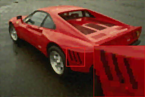
| Duck | Building | Hats | Car |
3.2 Experimental results
In order to verify the performance of our proposed model, we have tested the recovery results of gray images and color images under different blur kernels and different Gaussian noise levels. Tables 1, 2 and 3 show the values of PSNR, SSIM of the classic TV [38], DCA with [31], TRL2 [42], SOCF [28] and BM3D [15] on Gaussian blur and Motion blur and Average blur . The number in bold means the best result. Obviously, our algorithm gives the best results in most of the cases. We also show the average of PSNR/SSIM value of the restored image in the Table 4. Comprehensive evaluations on the image set with three kinds of kernels and four different noise levels demonstrate the superiority of our proposed method when compared with other state-of-the-art methods.
| PSNR/SSIM | Degraded | TV [38] | DCA [31] | TRL2 [42] | SOCF [28] | BM3D [15] | Ours |
|---|---|---|---|---|---|---|---|
| Shepp-Logan | 18.93/0.578 | 22.77/0.930 | 23.29/0.893 | 23.68/0.873 | 23.96/0.918 | 24.56/0.846 | 25.66/0.941 |
| Shape150 | 18.46/0.541 | 25.05/0.859 | 25.66/0.866 | 25.62/0.869 | 25.96/0.910 | 26.44/0.873 | 27.74/0.916 |
| House | 24.12/0.560 | 27.90/0.784 | 28.18/0.800 | 28.05/0.676 | 29.10/0.797 | 29.90/0.783 | 30.66/0.826 |
| Boat | 23.34/0.489 | 25.03/0.633 | 25.43/0.655 | 26.12/0.640 | 26.45/0.690 | 26.76/0.700 | 26.92/0.704 |
| Pepper | 21.41/0.573 | 23.46/0.735 | 23.69/0.736 | 24.71/0.705 | 24.87/0.781 | 26.42/0.763 | 25.86/0.793 |
| Cameraman | 20.87/0.499 | 23.10/0.716 | 23.49/0.734 | 24.16/0.645 | 24.24/0.745 | 24.74/0.737 | 24.73/0.758 |
| Hill | 24.85/0.497 | 26.86/0.631 | 27.12/0.653 | 27.35/0.644 | 27.55/0.670 | 28.07/0.688 | 28.08/0.693 |
| Plate | 17.40/0.779 | 21.64/0.910 | 21.92/0.916 | 21.90/0.912 | 22.71/0.923 | 24.57/0.942 | 24.84/0.947 |
| Duck | 24.17/0.659 | 27.00/0.789 | 27.13/0.804 | 27.25/0.742 | 28.11/0.823 | 28.60/0.830 | 29.13/0.834 |
| Building | 19.54/0.636 | 20.17/0.701 | 20.40/0.718 | 20.80/0.711 | 20.87/0.739 | 21.33/0.760 | 21.32/0.762 |
| Hats | 27.04/0.858 | 28.95/0.937 | 29.23/0.939 | 29.10/0.916 | 29.75/0.941 | 30.10/0.944 | 30.22/0.946 |
| Car | 23.92/0.755 | 25.18/0.828 | 25.70/0.838 | 26.03/0.819 | 26.22/0.841 | 26.74/0.847 | 26.98/0.853 |
| Average | 22.01/0.619 | 24.76/0.788 | 25.10/0.796 | 25.39/0.738 | 25.82/0.815 | 26.52/0.809 | 26.89/0.830 |
| PSNR/SSIM | Degraded | TV [38] | DCA [31] | TRL2 [42] | SOCF [28] | BM3D [15] | Ours |
|---|---|---|---|---|---|---|---|
| Shepp-Logan | 17.46/0.546 | 24.78/0.942 | 25.40/0.919 | 25.11/0.883 | 25.43/0.870 | 25.67/0.808 | 27.87/0.903 |
| Shape150 | 16.33/0.469 | 25.78/0.901 | 30.52/0.926 | 24.24/0.602 | 25.16/0.854 | 26.62/0.865 | 27.94/0.869 |
| House | 21.45/0.503 | 25.21/0.730 | 27.93/0.738 | 25.85/0.653 | 28.73/0.772 | 29.24/0.786 | 29.55/0.793 |
| Boat | 22.01/0.456 | 25.54/0.658 | 25.96/0.660 | 25.73/0.652 | 26.28/0.688 | 26.63/0.698 | 26.89/0.703 |
| Pepper | 20.06/0.532 | 23.94/0.763 | 24.16/0.732 | 23.44/0.665 | 24.86/0.772 | 25.39/0.768 | 24.79/0.755 |
| Cameraman | 19.80/0.478 | 23.92/0.736 | 24.50/0.705 | 24.41/0.612 | 24.91/0.739 | 25.25/0.745 | 25.29/0.746 |
| Hill | 23.21/0.451 | 26.61/0.632 | 26.88/0.642 | 26.72/0.639 | 26.98/0.655 | 27.42/0.670 | 27.50/0.675 |
| Plate | 15.93/0.730 | 20.99/0.902 | 21.55/0.911 | 21.19/0.903 | 23.09/0.932 | 24.11/0.941 | 24.44/0.953 |
| Duck | 22.48/0.623 | 26.79/0.782 | 26.81/0.782 | 26.61/0.683 | 27.98/0.792 | 28.03/0.808 | 28.57/0.797 |
| Building | 18.93/0.628 | 20.87/0.741 | 20.97/0.749 | 21.72/0.740 | 22.30/0.796 | 22.86/0.816 | 22.92/0.806 |
| Hats | 25.44/0.840 | 28.74/0.934 | 28.78/0.935 | 28.31/0.885 | 29.29/0.927 | 29.22/0.930 | 29.62/0.931 |
| Car | 22.05/0.737 | 24.97/0.830 | 25.57/0.838 | 25.56/0.803 | 25.82/0.841 | 26.49/0.843 | 26.89/0.844 |
| Average | 20.43/0.583 | 24.85/0.796 | 25.75/0.795 | 24.91/0.710 | 25.90/0.803 | 26.41/0.807 | 26.84/0.815 |
| PSNR/SSIM | Degraded | TV [38] | DCA [31] | TRL2 [42] | SOCF [28] | BM3D [15] | Ours |
|---|---|---|---|---|---|---|---|
| Shepp-Logan | 18.65/0.708 | 24.39/0.947 | 25.82/0.926 | 24.94/0.853 | 24.73/0.938 | 25.71/0.884 | 27.35/0.951 |
| Shape150 | 18.16/0.612 | 26.25/0.900 | 28.48/0.933 | 27.97/0.946 | 27.46/0.941 | 28.01/0.928 | 28.97/0.918 |
| House | 23.96/0.618 | 29.09/0.807 | 29.44/0.823 | 29.61/0.768 | 30.45/0.825 | 31.47/0.836 | 31.60/0.837 |
| Boat | 23.23/0.521 | 25.82/0.662 | 26.59/0.703 | 27.12/0.708 | 27.23/0.721 | 28.06/0.751 | 28.14/0.751 |
| Pepper | 21.25/0.613 | 24.21/0.763 | 25.45/0.781 | 25.78/0.777 | 27.02/0.823 | 27.75/0.806 | 27.89/0.820 |
| Cameraman | 20.70/0.561 | 23.87/0.743 | 24.47/0.766 | 24.78/0.642 | 24.66/0.704 | 25.81/0.781 | 25.98/0.792 |
| Hill | 24.85/0.528 | 27.46/0.661 | 28.03/0.695 | 28.39/0.709 | 28.43/0.708 | 29.03/0.731 | 28.96/0.736 |
| Plate | 17.08/0.766 | 22.98/0.930 | 23.86/0.941 | 23.54/0.935 | 25.04/0.950 | 26.19/0.958 | 26.80/0.963 |
| Duck | 24.12/0.709 | 28.43/0.821 | 28.59/0.837 | 29.21/0.845 | 29.34/0.850 | 29.91/0.863 | 30.62/0.863 |
| Building | 19.47/0.650 | 20.70/0.734 | 20.87/0.750 | 21.02/0.749 | 21.48/0.778 | 22.06/0.794 | 22.00/0.794 |
| Hats | 27.38/0.897 | 29.83/0.945 | 29.86/0.945 | 30.02/0.935 | 31.63/0.952 | 31.34/0.954 | 31.53/0.955 |
| Car | 23.93/0.785 | 26.40/0.847 | 26.43/0.850 | 26.49/0.843 | 27.16/0.859 | 27.41/0.861 | 27.67/0.863 |
| Average | 21.90/0.664 | 25.79/0.813 | 26.49/0.829 | 26.57/0.768 | 27.05/0.837 | 27.73/0.846 | 28.13/0.854 |
| Kernel | Degraded | TV [38] | DCA [31] | TRL2 [42] | SOCF [28] | BM3D [15] | Ours | |
|---|---|---|---|---|---|---|---|---|
| 22.22/0.678 | 27.30/0.838 | 26.91/0.821 | 26.26/0.785 | 27.40/0.845 | 27.46/0.836 | 27.82/0.857 | ||
| 22.00/0.619 | 24.76/0.789 | 25.10/0.796 | 25.40/0.762 | 25.82/0.812 | 26.52/0.809 | 26.81/0.831 | ||
| 22.37/0.527 | 25.37/0.791 | 24.96/0.770 | 24.03/0.727 | 25.57/0.789 | 25.65/0.786 | 25.97/0.811 | ||
| 21.15/0.472 | 25.17/0.771 | 24.63/0.765 | 24.18/0.721 | 25.16/0.775 | 25.24/0.776 | 25.74/0.796 | ||
| 20.58/0.638 | 27.75/0.819 | 28.03/0.829 | 26.93/0.812 | 27.41/0.834 | 27.70/0.834 | 28.09/0.846 | ||
| 20.43/0.583 | 24.84/0.793 | 25.75/0.795 | 24.91/0.727 | 25.90/0.799 | 26.41/0.807 | 26.86/0.815 | ||
| 20.10/0.496 | 25.26/0.768 | 25.10/0.757 | 23.51/0.737 | 24.94/0.760 | 25.24/0.780 | 25.75/0.783 | ||
| 19.82/0.445 | 24.58/0.757 | 24.63/0.763 | 23.56/0.696 | 24.46/0.755 | 24.69/0.768 | 25.25/0.776 | ||
| 21.90/0.664 | 25.79/0.813 | 26.49/0.829 | 26.57/0.793 | 27.05/0.837 | 27.73/0.846 | 28.13/0.854 | ||
| 21.70/0.605 | 26.41/0.812 | 26.07/0.811 | 24.89/0.730 | 26.65/0.816 | 26.76/0.819 | 27.16/0.831 | ||
| 21.26/0.515 | 25.61/0.792 | 25.12/0.776 | 24.37/0.737 | 25.71/0.783 | 25.87/0.793 | 26.24/0.809 | ||
| 20.87/0.462 | 25.12/0.767 | 24.72/0.756 | 24.12/0.726 | 25.63/0.793 | 25.44/0.781 | 25.84/0.798 |
| Kernel | TV [38] | DCA [31] | TRL2 [42] | SOCF [28] | BM3D [15] | Ours | |
|---|---|---|---|---|---|---|---|
| gray | 2.93 | 50.07 | 7.05 | 12.99 | 5.73 | 20.22 | |
| RGB | 12.96 | 162.96 | 31.44 | 60.56 | 27.94 | 79.28 | |
| gray | 2.46 | 60.61 | 10.90 | 17.03 | 5.81 | 20.52 | |
| RGB | 12.89 | 137.92 | 30.74 | 93.01 | 28.69 | 100.66 | |
| gray | 2.91 | 44.39 | 11.82 | 12.47 | 5.64 | 14.67 | |
| RGB | 12.76 | 152.73 | 36.67 | 62.05 | 28.21 | 85.09 |
 |
 |
 |
 |
|
| (a) Original image | (b) Degraded image | (c) TV [38] | (d) DCA [31] | |
| 18.74/0.398 | 24.04/0.804 | 23.11/0.823 | ||
 |
 |
 |
 |
|
| (e) TRL2 [42] | (f) SOCF [28] | (g) BM3D [15] | (h) Ours | |
| 23.44/0.773 | 23.93/0.827 | 23.76/0.833 | 24.83/0.929 |
 |
 |
 |
 |
|
| (a) Original image | (b) Degraded image | (c) TV [38] | (d) DCA [31] | |
| 17.12/0.765 | 22.06/0.915 | 21.62/0.910 | ||
 |
 |
 |
 |
|
| (e) TRL2 [42] | (f) SOCF [28] | (g) BM3D [15] | (h) Ours | |
| 20.10/0.868 | 22.23/0.914 | 22.77/0.920 | 23.30/0.928 |
 |
 |
 |
 |
|
| (a) Original image | (b) Degraded image | (c) TV [38] | (d) DCA [31] | |
| 23.43/0.499 | 28.15/0.703 | 28.04/0.704 | ||
 |
 |
 |
 |
|
| (e) TRL2 [42] | (f) SOCF [28] | (g) BM3D [15] | (h) Ours | |
| 27.70/0.692 | 28.36/0.712 | 28.53/0.717 | 28.56/0.722 |
 |
 |
 |
 |
|
| (a) Original image | (b) Degraded image | (c) TV [38] | (d) DCA [31] | |
| 22.48/0.623 | 26.79/0.782 | 27.36/0.793 | ||
 |
 |
 |
 |
|
| (e) TRL2 [42] | (f) SOCF [28] | (g) BM3D [15] | (h) Ours | |
| 26.61/0.683 | 27.98/0.792 | 28.03/0.808 | 28.57/0.797 |
 |
 |
 |
 |
|
| (a) Original image | (b) Degraded image | (c) TV [38] | (d) DCA [31] | |
| 23.70/0.543 | 29.60/0.798 | 28.76/0.802 | ||
 |
 |
 |
 |
|
| (e) TRL2 [42] | (f) SOCF [28] | (g) BM3D [15] | (h) Ours | |
| 26.80/0.592 | 29.75/0.796 | 30.33/0.808 | 30.49/0.817 |
 |
 |
 |
 |
|
| (a) Original image | (b) Degraded image | (c) TV [38] | (d) DCA [31] | |
| 23.10/0.685 | 26.14/0.834 | 25.56/0.825 | ||
 |
 |
 |
 |
|
| (e) TRL2 [42] | (f) SOCF [28] | (g) BM3D [15] | (h) Ours | |
| 25.18/0.799 | 25.95/0.823 | 26.24/0.839 | 26.54/0.842 |
In order to further demonstrate the superiority of our algorithm on image restoration more intuitively, we compare the visual quality of restored images of our proposed method and other state-of-the-art methods. We also zoom in key parts of the image for better illustrating. Figures show that our method yields the best image quality in terms of removing noise, preserving edges, and maintaining image sharpness. Looking carefully at the details in the figures, we can see that TV [38] oversmoothes images, TRL2 [42] introduces staircase effect, DCA [31] sharpens edges but loses some detail information, there exits the ringing phenomenon by SOCF [28] and BM3D model [15] introduces some artifacts.
Table 5 lists the computation time on a desktop (Intel(R) Core(TM) i5-8250 CPU @1.60 GHz), which reveal that our method is faster than DCA [31], but is slower than TV [38], BM3D [15], TRL2 [42] and SOCF [28]. Acceleration will be considered in the future work.
In brief, our algorithm (EAHR) has competitive performance in sharpening the edges and removing the noise, which outperforms other mainstream methods both in PSNR/SSIM values and visual quality.
4 Conclusion
For an entire image, the spatially fixed regularization parameters can not perform well for both edges and smooth areas. The larger parameters are favorable to reduce the noise in the smooth area, while incurs blur to edges. The small parameters enable regularization-based algorithms to sharpen the edges, but the denoising may not be sufficient.
In this paper, we have presented an automated spatially dependent regularization parameter selection framework for restoring an image from a noisy and blur image. An edge detector with high robustness to noise is used to detect the edges of the image and then generates an edge information matrix. According to this matrix, the automated spatially dependent parameters for regularization are given in binarization. With the help of these parameters, the regularization algorithm performs outstandingly at both edges and smooth areas. Once automated spatially dependent parameters are fixed, the proposed model is convex and therefore can be solved by sPADMM with a linear-rate convergence rate. Extensive experiments on different types of blurring kernels and different levels of Gaussian noise have been conducted to show that our approach is robust and outperforms other state-of-the-art deblurring methods. In addition, the proposed model not only effectively overcomes the false edges and staircase effects but also makes up for the insufficiency of the harmonic model’s diffusion in all directions and protects the edge well to restore the internal smooth area. Due to the limited space, we only display the experimental results in three cases: Gaussian blur , Motion blur and Average blur . The future work will include:
-
1.
We will accelerate our algorithm to reduce the recovery time.
-
2.
To remain more image details, we will examine an edge detector with higher accuracy and robustness. Moreover, the automated spatially dependent parameters will be considered according to the image texture.
-
3.
Our model is now only suitable for non-blind deblurring, and we will extend it to blind deblurring task.
Acknowledgement
The work has been supported by the National Natural Science Foundation of China (Grants Nos. 12061052), Natural Science Fund of Inner Mongolia Autonomous Region (Grant No. 2020MS01002), the China Scholarship Council for a one year visiting at Ecole Normale Supérieure Paris-Saclay (No. 201806810001). The authors would like to thank Professor Guoqing Chen for providing us some useful suggestions and this work is also partly supported by his project (“111 project”of higher education talent training in Inner Mongolia Autonomous Region).
Appendix. Convergence proof
To make the paper self-contained, we establish the global convergence result of algorithm 1.
Let , and . If is an optimal solution of (2.6) if and only if there exists Lagrange multiplier such that
where and is the subdifferential of . From the KKT conditions, we know that if is the KKT point of (2.6), then
| (4.1) |
Since the subdifferential mapping of the closed convex function is maximal monotone, there exist self-adjoint and positive semidefinite operators such that for all and ,
| (4.2) |
for all and ,
| (4.3) |
It is obtained by our algorithm that
| (4.4) |
Let . Denote , similarly ,
Therefore,
Noting (4.1), (4.2), (4.3) and (4.4), we find
| (4.5) |
| (4.6) |
By calculation, we get
Thus, (4.5) is converted to (4.7) and (4.6) becomes (4.8),
| (4.7) |
| (4.8) |
Then through (4.7) and (4.8), we obtain
| (4.9) |
Next, we shall estimate the term . It follows from equation (4.4) that
In addition, by the the maximal monotonic property of , we have
Let , then
| (4.10) |
Since , it follows from (4.9) and (4.10) that
| (4.11) |
Define
| (4.12) |
Next, we discuss two cases:
Case I: . It is obvious that
By the definition of and (4.11), we see
| (4.13) |
Case II: . Similarly, we have
| (4.14) |
Denote
Thus, from (4.13) and (4.14), we conclude that the sequence is bounded and monotonically decreasing, hence, it has limits. Since , the sequence is bounded.
Let or . Furthermore, from (4.13) and (4.14),
Thus,
| (4.15) |
| (4.16) |
Considering the relationship , we have . By (4.15) and the bounded property of , one can get these sequences , , , , are bounded. By using the inequality
we deduce that is bounded, so is bounded. Since , and the positive definite property of , the sequence is bounded, and hence the sequence is bounded. Therefore, the sequence is bounded, which implies the existence of a convergent subsequence to a clusters point, denoted as .
It follows from (4.12) and (4.15) that
| (4.17) |
Thus, from
we have . Taking limits on both sides of equation (4.4) along the subsequence and using the closedness of subdifferential, we have
Thus, is the optimal solution of (2.6) and is the corresponding Lagrange multiplier.
Now, let’s prove that . Since satisfies (4.4), we could replace with in the above analysis. From (4.13), (4.14), (4.15) and (4.16), we find . (4.13) and (4.14) indicate the sequence has limits, then . So . Further, we know by the definition of that
| (4.18) |
Considering (4.15) and (4.16), we get
| (4.19) |
| (4.20) |
From the positive semidefinite property of and the positive definite property of , it is clear that
which combined with (4.20) gives , namely, .
In brief, when , we have
References
References
- [1] R. Acar and C. Vogel. Analysis of bounded variation penalty methods for ill-posed problems. Inverse Problems, 10:1217–1229, 1994.
- [2] A. Almansa, C. Ballester, V. Caselles, and G. Haro. A tv based restoration model with local constraints. Journal of Scientific Computing, 34(3):209–236, 2008.
- [3] F. Benvenuto, A La Camera, C. Theys, A. Ferrari, H Lantéri, and M. Bertero. The study of an iterative method for the reconstruction of images corrupted by poisson and gaussian noise. Inverse Problems, 24(3):35016–35020, 2008.
- [4] M. Bertalmio, V. Caselles, B. Rougé, and A. Solé. Tv based image restoration with local constraints. Journal of Scientific Computing, 19:95–122, 2003.
- [5] Stephen Boyd, Neal Parikh, Eric Chu, Borja Peleato, and Jonathan Eckstein. Distributed optimization and statistical learning via the alternating direction method of multipliers. Foundations & Trends in Machine Learning, 3(1):1–122, 2010.
- [6] Jian Feng Cai, Raymond H. Chan, and Mila Nikolova. Two-phase approach for deblurring images corrupted by impulse plus gaussian noise. Inverse Problems and Imaging, 2(2):187–204, 2008.
- [7] Jian Feng Cai, Raymond H. Chan, and Mila Nikolova. Fast two-phase image deblurring under impulse noise. Journal of Mathematical Imaging and Vision, 36(1):46–53, 2010.
- [8] Jian Feng Cai, Bin Dong, Stanley Osher, and Zuowei Shen. Image restorations: Total variation, wavelet frames, and beyond. Journal of the American Mathematical Society, 25(2):1033–1089, 2012.
- [9] Jian Feng Cai, Stanley Osher, and Zuowei Shen. Linearized bregman iterations for frame-based image deblurring. SIAM Journal on Imaging Sciences, 2(1):226–252, 2009.
- [10] Jian Feng Cai, Stanley Osher, and Zuowei Shen. Split bregman methods and frame based image restoration. SIAM Journal on Multiscale Modeling & Simulation, 8(2):337–369, 2009.
- [11] Antonin Chambolle. An algorithm for total variation minimization and applications. Journal of Mathematical Imaging and Vision, 20:89–97, 2004.
- [12] Dali Chen, Shenshen Sun, Congrong Zhang, Yang Quan Chen, and Dingyu Xue. Fractional-order tv-l2 models for image denoising. Central European Journal of Physics, 11(10):1414–1422, 2013.
- [13] Kostadin Dabov, Alessandro Foi, Vladimir Katkovnik, and Karen Egiazarian. Color image denoising via sparse 3d collaborative filtering with grouping constraint in luminance-chrominance space. In 2007 IEEE International Conference on Image Processing, volume 1, pages I–313. IEEE, 2007.
- [14] Kostadin Dabov, Alessandro Foi, Vladimir Katkovnik, and Karen Egiazarian. Image denoising by sparse 3-d transform-domain collaborative filtering. IEEE Transactions on image processing, 16(8):2080–2095, 2007.
- [15] Kostadin Dabov, Alessandro Foi, Vladimir Katkovnik, and Karen O. Egiazarian. Image restoration by sparse 3d transform-domain collaborative filtering. 2008.
- [16] Yiqiu Dong, Torsten GöRner, and Stefan Kunis. An algorithm for total variation regularized photoacoustic imaging. Advances in Computational Mathematics, 41:423–438, 2015.
- [17] Yiqiu Dong, Michael Hintermüller, and M. Monserrat Rincon-Camacho. Automated regularization parameter selection in multi-scale total variation models for image restoration. Journal of Mathematical Imaging & Vision, 40(1):82–104, 2011.
- [18] Maryam Fazel, Ting Kei Pong, Defeng Sun, and Paul Tseng. Hankel matrix rank minimization with applications to system identification and realization. SIAM Journal on Matrix Analysis and Applications, 34(3):946–977, 2013.
- [19] Ali Gholami and S. Mohammad Hosseini. A balanced combination of tikhonov and total variation regularizations for reconstruction of piecewise-smooth signals. Signal Processing, 93(7):1945–1960, 2013.
- [20] Tom Goldstein and Stanley Osher. The split bregman method for l1 regularized problems. SIAM Journal on Imaging Sciences, 2(2):323–343, 2009.
- [21] Zheng Gong, Zuowei Shen, and Kim-Chuan Toh. Image restoration with mixed or unknown noises. SIAM Journal on Multiscale Modeling and Simulation, 12(2):458–487, 2014.
- [22] Deren Han, Defeng Sun, and Liwei Zhang. Linear rate convergence of the alternating direction method of multipliers for convex composite programming. Mathematics of Operations Research, 43(2):622–637, 2018.
- [23] Jie Huang, Marco Donatelli, and Raymond Chan. Nonstationary iterated thresholding algorithms for image deblurring. Inverse Problems and Imaging, 7(3):717–736, 2013.
- [24] Yumei Huang, Michael K.Ng, and You-Wei Wen. A fast total variation minimization method for image restoration. SIAM Journal on Multiscale Modeling and Simulation, 7(2):774–795, 2008.
- [25] Tongtong Jia, Yuying Shi, Yonggui Zhu, and Lei Wang. An image restoration model combining mixed l1/l2 fidelity terms. Journal of Visual Communication and Image Representation, 38:461–473, 2016.
- [26] Fang Li, Chaomin Shen, Jingsong Fan, and Chunli Shen. Image restoration combining a total variational filter and a fourth-order filter. Journal of Visual Communication and Image Representation, 18(4):322–330, 2007.
- [27] Min Li, Defeng Sun, and Kim-Chuan Toh. A majorized admm with indefinite proximal terms for linearly constrained convex composite optimization. SIAM Journal on Optimization, 26(2):922–950, 2016.
- [28] Jingjing Liu, Yifei Lou, Guoxi Ni, and Tieyong Zeng. An image sharpening operator combined with framelet for image deblurring. Inverse Problems, 36(4), 2020.
- [29] Kui Liu, Jieqing Tan, and Liefu Ai. Hybrid regularizers-based adaptive anisotropic diffusion for image denoising. SpringerPlus, 5(1):1–24, 2016.
- [30] Kui Liu, Jieqing Tan, and Benyue Su. An adaptive image denoising model based on tikhonov and tv regularizations. Advances in Multimedia, 2014:1–10, 2014.
- [31] Yifei Lou, Tieyong Zeng, Stanley Osher, and Jack Xin. A weighted difference of anisotropic and isotropic total variation model for image processing. SIAM Journal on Imaging Sciences, 8(3):1798–1823, 2015.
- [32] Marius Lysaker, Arvid Lundervold, and Xue-cheng Tai. Noise removal using fourth-order partial differential equation with applications to medical magnetic resonance images in space and time. IEEE Transactions on Image Processing, 12(12):1579–1590, 2003.
- [33] Liyan Ma, Li Xu, and Tieyong Zeng. Low rank prior and total variation regularization for image deblurring. Journal of Scientific Computing, 70:1336–1357, 2017.
- [34] Jitendra M. Malik and Pietro Perona. Scale-space and edge detection using anisotropic diffusion. IEEE Transactions on Pattern Analysis and Machine Intelligence, 12(7):629–639, 1990.
- [35] Jin Jin Mei, Yiqiu Dong, and Ting Zhu Huang. Simultaneous image fusion and denoising by using fractional-order gradient information. Journal of Computational and Applied Mathematics, 351:212–227, 2018.
- [36] Mario Micheli, Yifei Lou, Stefano Soatto, and Andrea L. Bertozzi. A linear systems approach to imaging through turbulence. Journal of Mathematical Imaging and Vision, 48:185–201, 2014.
- [37] Seungmi Oh, Hyenkyun Woo, Sangwoon Yun, and Myungjoo Kang. Non-convex hybrid total variation for image denoising. Journal of Visual Communication and Image Representation, 24(3):332–344, 2013.
- [38] Leonid I. Rudin, Stanley Osher, and Emad Fatemi. Nonlinear total variation based noise removal algorithms. Physica D-Nonlinear Phenomena, 60(1-4):259–268, 1992.
- [39] Andrej Nikolaevich Tikhonov and Vasiliy Yakovlevich Arsenin. Solution of ill-posed problems. Mathematics of Computation, 32(144):266–267, 1977.
- [40] Yilun Wang, Junfeng Yang, Wotao Yin, and Yin Zhang. A new alternating minimization algorithm for total variation image reconstruction. SIAM Journal on Imaging Sciences, 1(3):248–272, 2008.
- [41] Zhou Wang, Alan Conrad Bovik, Hamid Rahim Sheikh, and Eero P. Simoncelli. Image quality assessment: from error visibility to structural similarity. IEEE Transactions on Image Processing, 13(4):600–612, 2004.
- [42] Chunlin Wu, Zhifang Liu, and Shuang Wen. A general truncated regularization framework for contrast-preserving variational signal and image restoration: Motivation and implementation. Science China Mathematics, 61(9):1711–1732, 2018.
- [43] Chunlin Wu and Tai Xue-Cheng. Augmented lagrangian method, dual methods, and split bregman iteration for rof, vectorial tv, and high order models. SIAM Journal on Imaging Sciences, 3(3):300–339, 2010.
- [44] Tingting Wu, Wei Li, Lihua Li, and Tieyong Zeng. A convex variational approach for image deblurring with multiplicative structured noise. IEEE Access, 8:37790–37807, 2020.
- [45] Xiongjun Zhang, Minru Bai, and Michael K. Ng. Nonconvex-tv based image restoration with impulse noise removal. Siam Journal on Imaging Sciences, 10(3):1627–1667, 2017.
- [46] Shixiu Zheng, Zhenkuan Pan, Guodong Wang, and Xu Yan. A variational model of image restoration based on first and second order derivatives and its split bregman algorithm. pages 860–865, 2012.